Suggested uses of the simulator #1

This section describes a sample scenario comparison and one way to use it.  Pitting it against real life is a bit iffy because the computer simulation simply does not come anywhere close to replicating all of the events that occur in an individual baseball game with player substitutions, errors, etc…  It’s best to pit two scenarios against each other.  The model, as currently constituted, is not particularly sophisticated but if you pit two scenarios against each other, I believe you can assume that a lot of the error washes out, particularly if the scenarios are close to one another.  For example, you can vary one player to see how much their performance matters or maybe check lineup sequences.  You can play with lineups. You can do whatever you dream up.

I’m going to outline a sample study of bunting strategies.  In this situation, we want to run a comparative analysis concerning the question of whether bunting the number two spot after the first hitter gets on is a good idea or a bad idea in terms of run generated in the inning.

So the idea would be first to assemble your roster and batting order.  I’m going to use the ‘hot’ 2014 Pittsburgh Pirates which doesn’t include their very cold April and May of that year.  You could argue pros and cons of that but the good news is that if you want to include those ABs, simply redo the At Bat data from Fangraphs, re-generate the PID profiles, and rerun the analysis.  It’s all up to you.  

So, here is the lineup I’m using for this analysis:

Josh Harrison

Starling Marte

Andrew McCutchen

Neil Walker

Russell Martin

Travis Snider (aka, ‘good’ Snider)

Ike Davis

Jorday Mercer 

pitcher

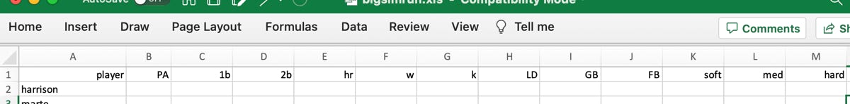
Next start collecting results.  I usually start by putting a list of the players I want to use in a spreadsheet that looks something like this:

I have a column for each of the figures I’ll need for the Quick Profile Generator.  Also I include a couple of more columns and add in batting average, OBP and slugging percentage to make it easier to use the Quick Profile Generator cumulative stat cross checks.

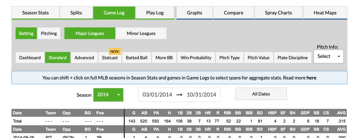
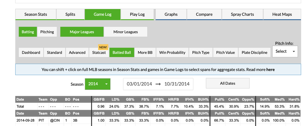
Next I head over the Fangraphs and pull the necessary data by looking up the player (Josh Harrison to start), pulling up the game log for the time period in question (2014), and transferring info from the summary lines for the ‘dashboard’ and ‘batted ball’ data blocks.

As you can see, you can get the hits and At Bat information from the first view and the batted ball info from the second view.   As an important note, use Plate Appearance and no At Bats as the total number of player appearances.   Jot those numbers in to the spreadsheet and then pull up the next players data.  Advance player by player through your spreadsheet until you have filled it out.

A note here.  It is not necessary to collect batting average and other collateral stats but it help when trying to validate runs during in the Quick Profile Generator.

For the pitchers I’ve recorded an automatic strike out.  It probably isn’t going to matter because the comparison will be from the top of the order and won’t matter much at that point.

Next step is to enter the data one player at a time into the Quick Profile Generator, calculate and cross check the entered values, and then save the data into a newly created PID file.  You can see the details for doing that in the Detail Guides section of the website.  

So, there will be several side by side runs.  In the first pair of runs, we assume a runner (Josh Harrison) is on first and the rest of the inning follows.  First run has Marte bunt and Harrison is on second and now there is one out with Cutch up.  Second run has Marte swinging away with no outs.  The analysis assumes that the sacrifice will be 100 percent successful.  You can argue with that if you want but I’m not going to right now.

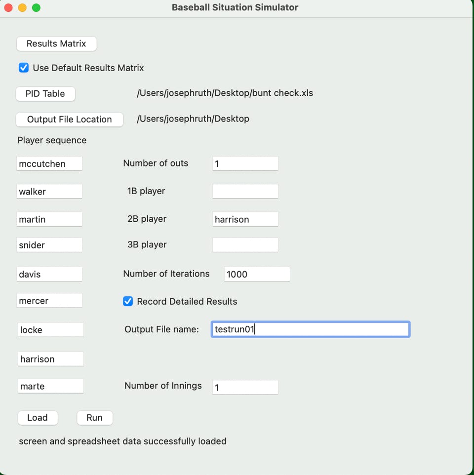
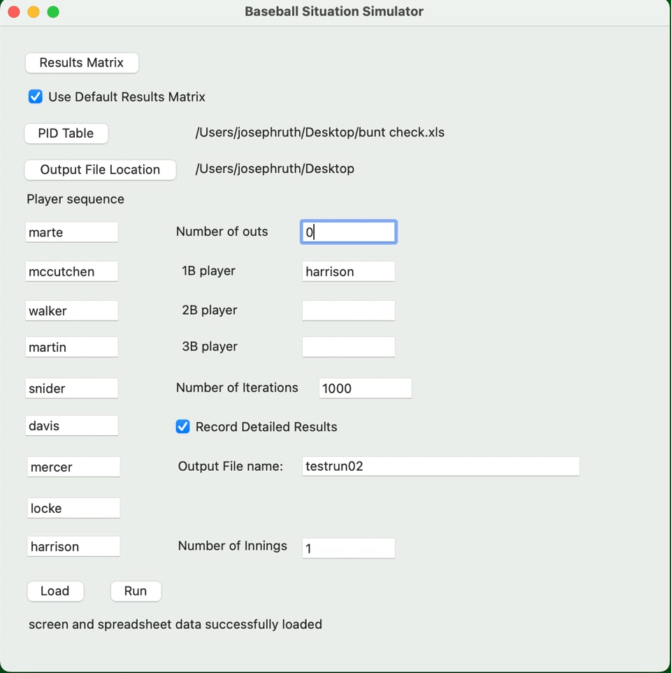
So I have all of my PID files and result file ready and am going to set up the first run which looks like this:

So you can see in this run that we’re assuming one out with Harrison on second (meaning the sacrifice was successful) and we’ll run it 1000 times and we’ll save the outcome in a file named ‘bunt check scenario 1’ saved on the Desktop.

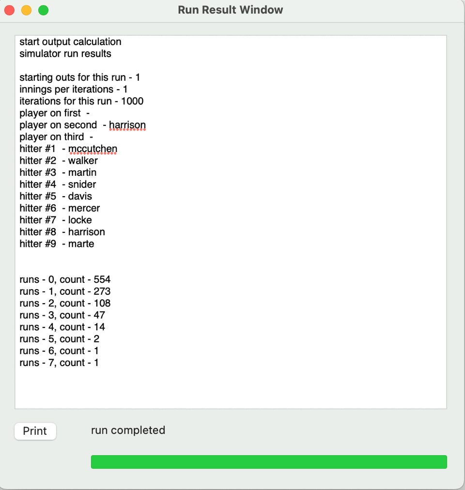
Pressed the ‘Load’ button and got the ‘screen and spreadsheet successfully loaded’ message and then pressed run, various run in progress status screens show up and then you see the following:

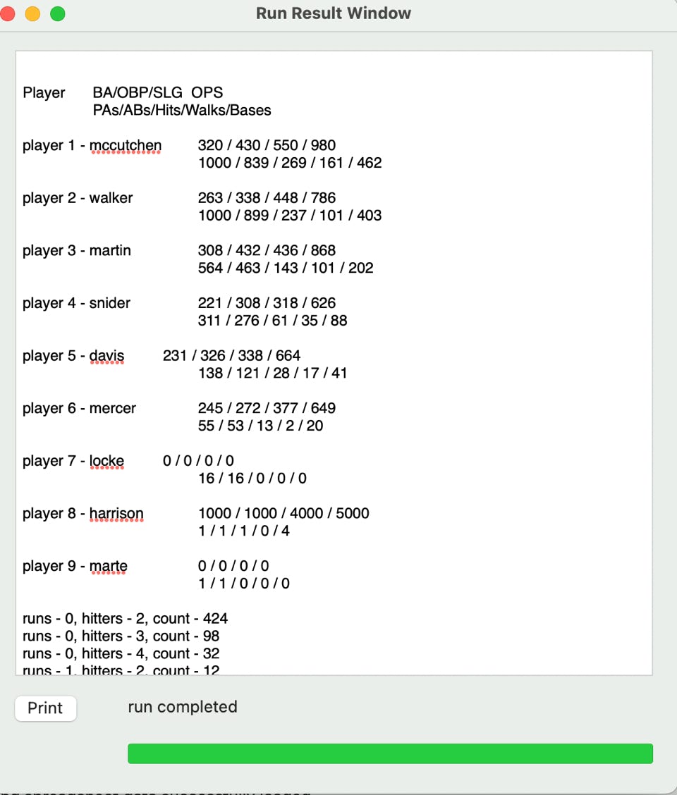
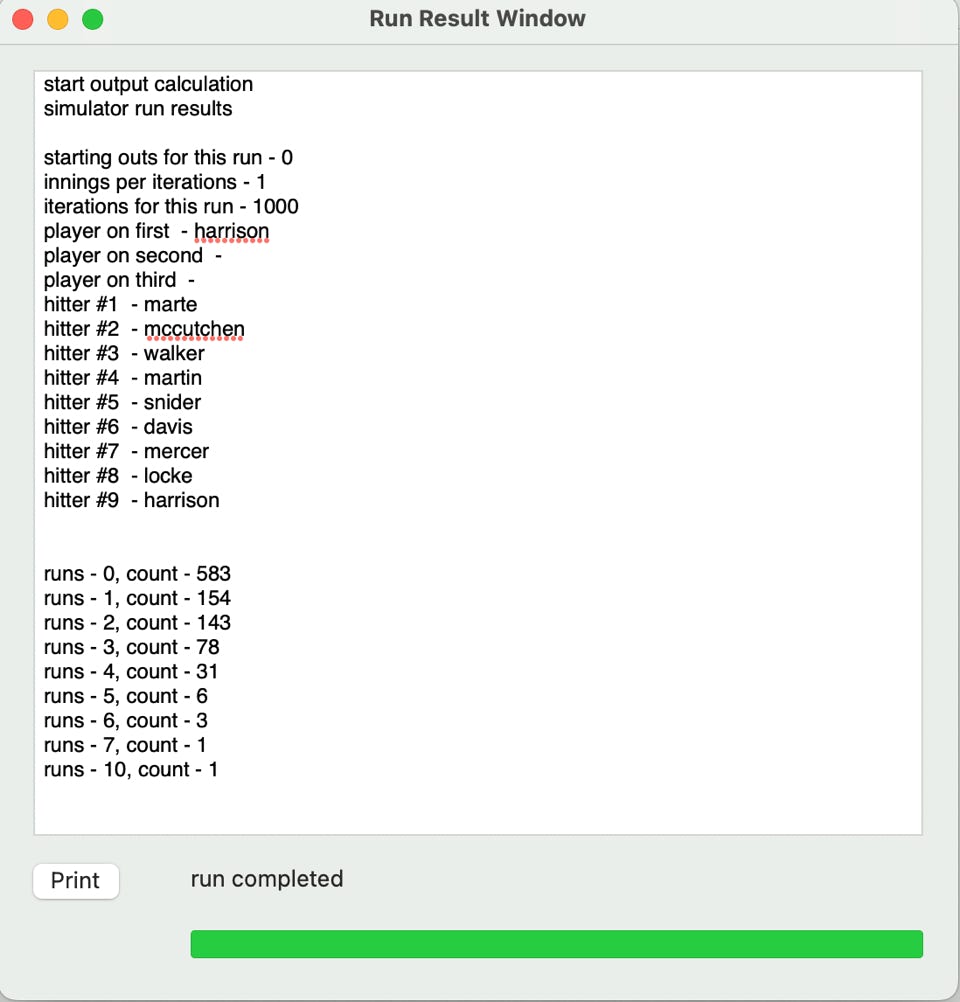
The resulting output screen first shows what screen settings went into the run and some of the results. Scroll down a bit and you get more information.

You see the cumulative batting average results to review as your sanity check.  These seem high to me so probably need to review the input data but this is just a sample run to shows features and how you might use the sanity check.

run 0 = 554 

run 1 = 273

run 2+ = 173

So now let’s redo this without the bunt and see what we get:

This one sets up a little differently with no outs, Harrison first, and the lineup shifted up two positions.  Loaded the spreadsheet and now hit the ‘run’ button:

The run distribution is a little different. 

run 0 = 583 

run 1 = 154

run 2+ = 263 

So... according to this little simulation process, it seems to indicate that with this lineup that bunting bumps down the probability of scoring a single run but increasing the possibility of scoring multiple runs.  Moving this situation down into the lineup to less capable hitters probably skews this even further.  It kind of indicates that the only time with this particular lineup that you want the second hitter bunting is if the first run you score wins the game.

To be sure, you mileage may vary if you move this situation up and down the lineup.  Harrison at second with one out with McCutchen, Walker, and Martin coming up is NOT the same as Walker on second with Snider, Ike Davis, and Mercer following.  Also you can grind in the fact that sacrifice bunts are not 100 percent successful by splitting the run at various percentage point breaks and figuring out where the tipping point is located.