PCA Tutorial

The purpose of this tutorial is to walk the new user through a PCA analysis beginning to end.

Those who have never used H₂O before should see the quick start guide for additional instructions on how to run H₂O.

When to Use PCA

PCA is used to reduce dimensions and solve issues of multicollinearity in high dimension data.

Getting Started

This tutorial uses a publicly available data set that can be found at: http://archive.ics.uci.edu/ml/datasets/Arrhythmia

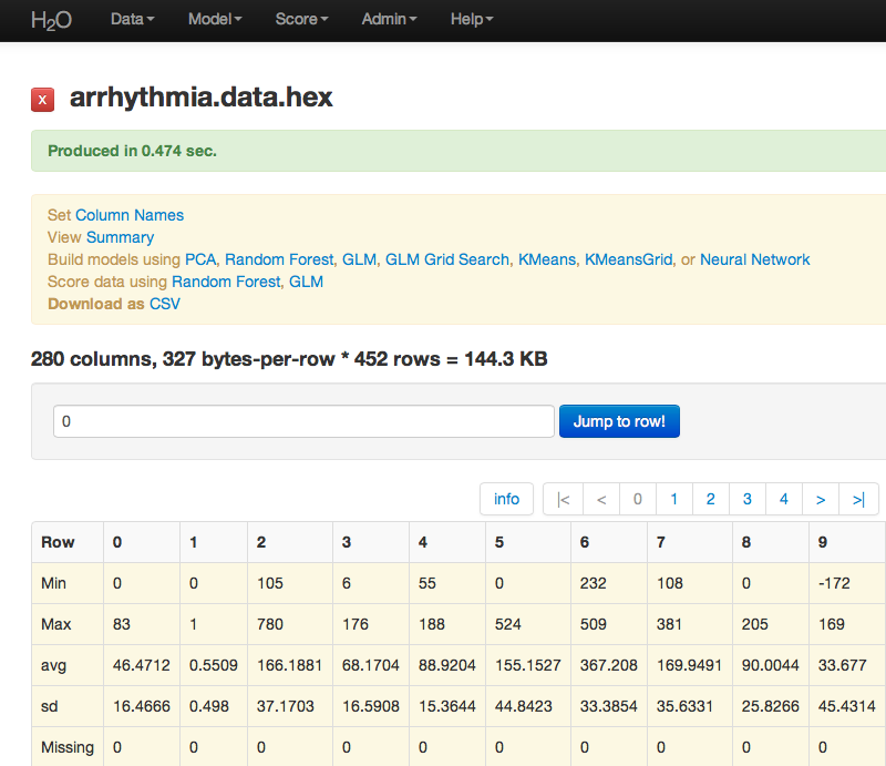
The original data are the Arrhythmia data set made available by UCI Machine Learning repository. They are composed of 452 observations and 279 attributes.

Before modeling, parse data into H₂O as follows:

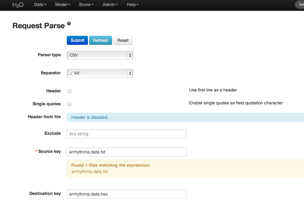
1. Under the drop down menu Data select Upload and use the helper to upload data.
2. User will be redirected to a page with the header “Request Parse”. Select whether the first row of the data set is a header. All other settings can be left in default. Press Submit.
3. Parsing data into H₂O generates a .hex key (“data name.hex”)

After parsing:

Building a Model

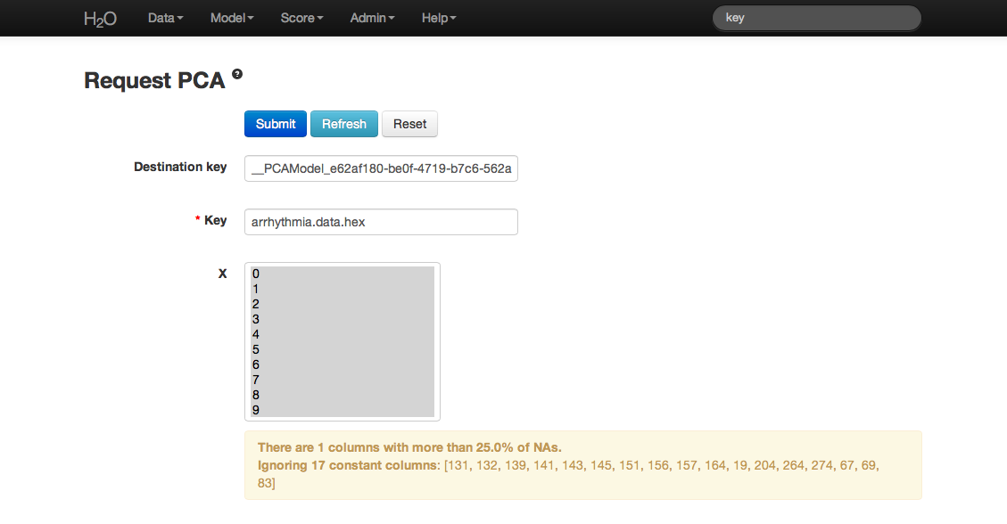
1. Once data are parsed a horizontal menu will appear at the top of the screen reading “Build model using ... ”. Select PCA here, or go to the drop down menu Model and select PCA.
2. In the Key field enter the .hex key for the Arrhythmia data set.
3. In the X field select the set of columns to be included in the components analysis. Note that PCA ignores categorical variables and constant columns.
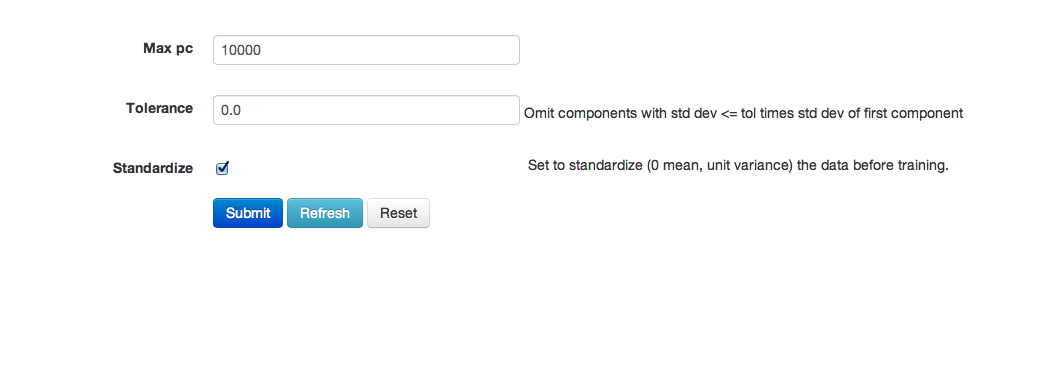
4. Specify MaxPC to be the maximum number of principal components to be returned.
5. Specify Tolerance so that components exhibiting low standard deviation (which indicates a lack of contribution to the overall variance observed in the data) are omitted. In this example we set Tolerance to 3.
6. Choose whether or not to standardize. Standardizing is highly recommended, as choosing to not standardize can produce components that are dominated by variables that appear to have larger variances relative to other attributes as a matter of scale.

Additional specification detail

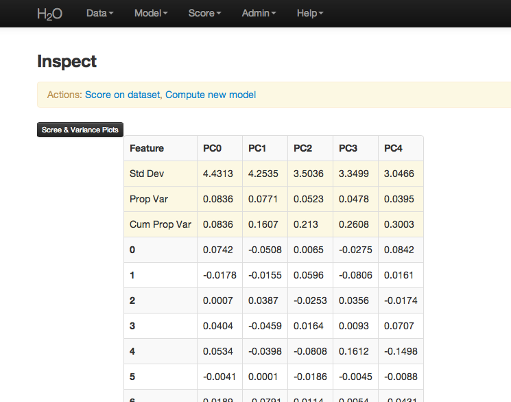
PCA Results

PCA output returns a table displaying the number of components indicated by whichever criteria was more restrictive in this particular case. In this example, a maximum of 5 components were requested, and a tolerance set to 3, so the first 5 components were returned.

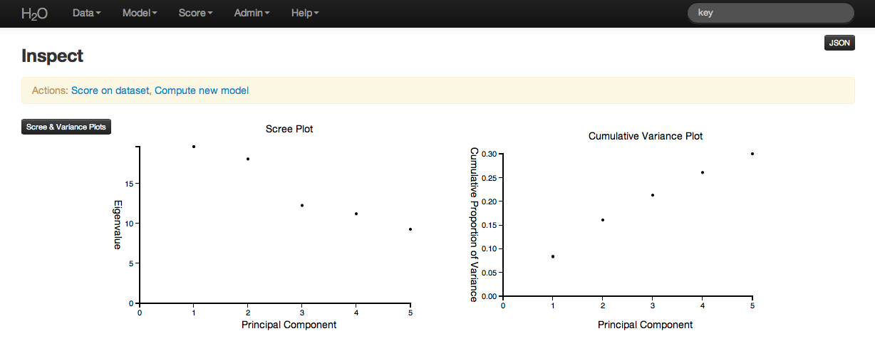
Scree and cumulative variance plots for the components are returned as well. Users can access them by clicking on the black button labeled “Scree and Variance Plots” at the top left of the results page. A scree plot shows the variance of each component, while the cumulative variance plot shows the total variance accounted for by the set of components.

Users should note that if they wish to replicate results between H₂O and R, it is recommended that standardization and cross validation either be turned off in H₂O, or specified in R.

THE END.