CS525 Project 3 - Sonar data raytracing using OpenCL

For this project I decided to work on one of the tasks we are currently udertaking as part of the ENDURANCE project.: sonar data raytracing using a sound speed model. This process is by nature extremely parallel (each sonar ping represents an independent beam to be raytraced), and can greatly benefit from the acceleration that GPU computation can offer.

Introduction

Multibeam sonar system theory is quite complex: What follows is a brief introduction of the aspects more related to this project. This intro has been taken from the MBSystem Cookbook. The Cookbook provides a lot of additional information about how sonars and sonar data processing.

How Sound Travels Through Water

The basic measurement of most sonar systems is the time it takes a sound pressure wave, emitted from some source, to reach a reflector and return. The observed travel time is converted to distance using an estimate of the speed of sound along the sound waves travel path. Estimating the speed of sound in water and the path a sound wave travels is a complex topic that is really beyond the scope of this cookbook. However, understanding the basics provides invaluable insight into sonar operation and the processing of sonar data, and so we have included an abbreviated discussion here.

Speed of Sound

The speed of sound in sea water is roughly 1500 meters/second. However the speed of sound can vary with changes in temperature, salinity and pressure. These variations can drastically change the way sound travels through water, as changes in sound speed between bodies of water, either vertically in the water column or horizontally across the ocean, cause the trajectory of sound waves to bend. Therefore, it is imperative to understand the environmental conditions in which sonar data is taken.

Affects of Temperature, Salinity and Pressure

The speed of sound increases with increases in temperature, salinity and pressure. Although the relationship is much more complex, to a first approximation, the following tables provides constant coefficients of change in sound speed for each of these parameters. Since changes in pressure in the sea typically result from changes in depth, values are provided with respect to changes in depth.

• Change in Speed of Sound per Change in Degree C ---> + 3 meters/sec
• Change in Speed of Sound per Change in ppt Salinity ---> + 1.2 meters/sec
• Change in Speed of Sound per Change in 30 Meters of Depth ---> + .5 meters/sec

Temperature has the largest effect on the speed of sound in the open ocean. Temperature variations range from 28 F near the poles to 90 F or more at the Equator. Of course, relevant temperature differences with regard to multibeam sonar systems are the variations that occur over relatively short distances, in particular those that occur with depth. These are discussed further below.
While the salinity of the world's oceans varies from roughly 32 to 38 ppt. These changes are gradual, such that within the range of a multibeam sonar, the impact on the speed of sound in the ocean is negligible. However near land masses or bodies of sea ice, salinity values can change considerably and can have significant effects on the way sound travels through water.
While the change in the speed of sound for a given depth change is small, in depth excursions where temperature and salinity are relatively constant, pressure changes as a result of increasing depth becomes the dominating factor in changes in the speed of sound.

The Sound Speed Profile

The composite effects of temperature, salinity and pressure are measured in a vertical column of water to provide what is known as the "sound speed profile or SSP . The SSP shown below has been generated using a Chen/Millero sound speed model over real data collected during the ENDURANCE 2009 mission: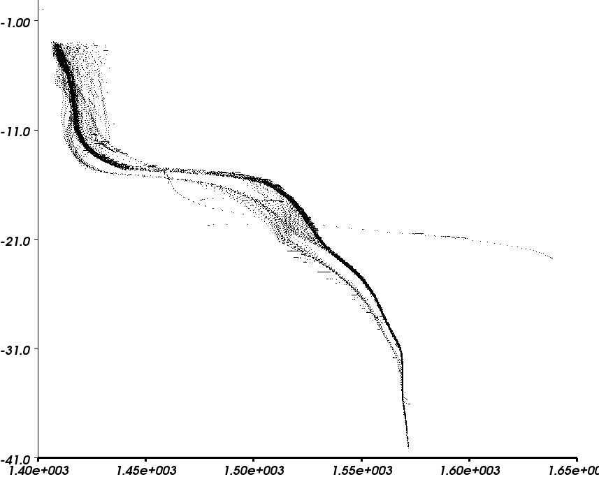 From this data a piecewise linear function is extracted, usually through simple done-by-hand fitting of a limited number of control points. It is this piecewise function that is actually going to be used for the raytracing. The more control points, the more separate layers we will have to raytrace sonar beams through: This raytracing calculation is needed because, as sonar beams go through layers of water with different densities (i.e. different sound speeds) they will be refracted at different angles.

Refraction

It is convenient, when talking about sound and its travel path from a point, to consider the path as a ray. This is a common technique in wave theory, used in optics and other sciences. In a homogeneous medium sound does indeed travel in a straight line. However, when a sound wave passes between two mediums having different sound speeds its direction is bent. This is a property of waves more than sound itself, and many theories and explanations, with varying degrees of success, have been put forth over they years. While not true in all cases a simple one for illustration is offered here.

Snell's Law

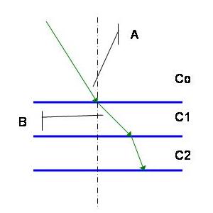
Consider sound wave incident on a boundary between two bodies of water having differing sound speeds as shown in the figure above. Snell's Law states that the Cosine of the initial angle of incidence divided by the initial sound speed is a constant as the sound passes from regions of differing sound speeds.

Cos (A) / Co = Constant

Therefore, if the new region has lower sound speed, the Cosine of the angle of incidence must be less than that of the previous region. Hence the new angle of incidence is less. So one might imagine the sound bending "toward" regions of lower sound speed, in the sense that the angle of sound travel is more steep, and "away" from regions of higher sound speed in the sense that the angle of incidence is more shallow.

Then if one knows the angle that a sound wave left its source, and the sound speed profile of the medium it passes through, one can calculate the path the wave takes over its entire trip.

A slightly more complicated example is one where the sound speed of a single medium changes linearly with depth rather than at discrete depth intervals. In this scenario, the sound ray bends continuously over its travel path. It can be shown that the path the sound travels is that of the arc of a circle whose radius, R, is the ratio of the initial sound speed and the slope of the gradient (R = Co/g)

Data Processing Steps

There are four main steps in the data processing pipeline built for this project:

FBT Data Loading

This step consists in loading the source sonar data and storing it in memory. The data is loaded from files using the fast bathymetry file format. This format was created by the Lamont-Doherty Earth Observatory and the Monterey Bay Aquarium Research Institute to serve as general purpose archive formats for processed swath data. The choice of this format is justified by the fact that the mbsystem toolset can convert almost any source sonar data format into this one, and all of the mbsystem tools (i.e. the data plotting utilities) can be used with this format.
A detailed description of the fast bathymetry file format can be found Here.

Takeoff angle and travel times computation

For each sonar beam, the raytracing algorithm needs the beam travel time and the angle at which it departed from the sonar transducer. This information is not directly present in the source data, since fast bathymetry just stores depth readings using the transducer position and the ship heading as a reference frame. This is a good format if we just want to visualize the data (is it straightforward to generate a 3d point cloud out of this information) but it is not what we need for the raytracing.
To compute the takeoff angles we use a polar shperical coordinate conversion. During this step we have to make sure the ship reference frame is correct (especially, the original depth has to be converted taking into accout the sonar transducer depth at the corresponding time, otherwise the angles will be incorrect). For the beam travel times, we simply compute the original beam length and use a nominal sound speed of 1500 meters per second ( the standard speed of sound in water).
IMPORTANT NOTE: This assumption may or may not be correct depending on how data was collected. This correction should be done using actual sound speed readings at the transducer source during data collection. If this information is available, it is easy to take it into account during the travel time computation.

Raytracing

This step performs the actual beam raytracing through a sound speed profile specified and loaded as a piecewise linear function. As a first (non parallelized step) gradients for the sound speed profile are computed. They will be used during the actual, parallel raytracing. As explained in previous sections, the raytracing algorithm takes into account both constant layers (where raytracing is linear) and non-zero gradient layers, where rays follow circular paths.
The raytracing code is derived directly from the mbsystem toolset raytracing functions.

FBT output writing

During this step, we simply generate an output file containing the processed data, in the same fast bathymetry format used for the input data.

Implementation

Program Structure

The program has been built as two separate modules: a C library (libfbt), containing most of the code, and a simple command-line executable using the library to process a single fbt file passed as a parameter, together with a SSP input file. This allows the future integration of the library into other applications (i.e. LookingGlass)

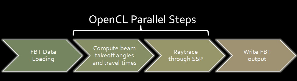
OpenCL Implementation

OpenCL was chosen over CUDA because it allows us to compile and execute kernels using CPU cores, if GPU acceleration is not available. This means that even without the appropriate drivers, we can still get a performance benefit parallelizing the computation on a multi core machine. With CUDA this is not possible: kernels can be executed only on CUDA-compatible GPUs. CUDA emulation mode requires a program recompilation and is just a debugging tool, not designed for production-grade performance: Emulated CUDA kernels actually run slower that corresponding sequential CPU code.

Kernels and Workgroup organization

The processing pipeline uses two separate kernels, one for the takeoff angle computation, and another one for the actual raytracing. The parallel workgroups are organized as follows:

• Each thread processes a single sonar beam.
• Thread blocks process all of the sonar beams generated by the transducer at a single point in time (a single ping): This is the most natural way to distribute work across processing units (and it is the way sonar data is normally organized): While the ship moves, multibeam sonar systems generate pings at a regular interval: each ping is constituted by a number of separate sonar beams. In other words, all of these sonar beams share some physical quantities (i.e. they have been generated at the same point in space), and it makes sense to process them all together inside a single thread block to possibly take advantage of data sharing for certain pieces of data (i.e. the sound speed profile, assuming we want to use multiple ones for different points in space).

The only limitation of the presented approach is that the number of beams generated during a single ping must not exceed the maximum number of threads per thread-block (i.e. 256). This is usually not the case, since most multibeam systems generate about 100 beams per ping. Otherwise, we can can still split ping processing across multiple thread blocks, by doing the right global / local thread id to beam index conversion.

Experimental results

The initial idea was testing the program using a part of East Lake Bonney bathymetry from ENDURANCE missions 2008 or 2009. Sadly this was not possible, since bathymetry data from the ENDURANCE missions needs some additional processing (i.e. navigation merging) before it is possible to convert it to the fast bathymetry format. As a fallback, I used data coming from the standard mbsystem data package: In particular I chose a chunk of sonar data coming from a 1998 survey of Lo'ihi Seamount, an underwater volcano located around 35 km (22 mi) off the southeast coast of the island of Hawaii.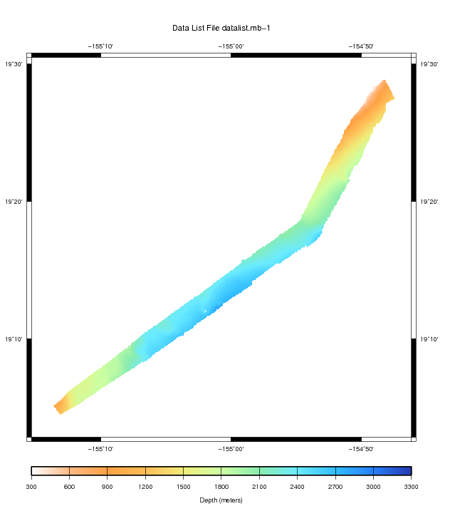
The single swath I considered is pretty small: 2400 pings of about 135 beams each, making up a total of 324'000 sonar beams. Still, this is enough to measure performance differences between standard and parallel implementations of the raytracing algorythm.

Performance

The parallel implementation has been measured to be about 40 times faster than the standard implementation. It is worth noting how the parallel code was not particularly optimized: I simply ported the mbsystem code in the most straightforward manner possible, to avoid breaking up something in the pretty complex raytracer.
I also suspect the bottleneck of the system right now lies in the memory transfer: the dataset may be too small to get a more significant performance gain out of the parallel implementation.

Errors

The two previous screenshots display two versions of the processed dataset: The one on the left is generated by the standard mbsystem tool, the left one has been created by the parallel raytracer. No large scale differences are evident but looking more in detail it is possible to see some slight differences in the data contours, as the two following images show: I suspect these differences derive by the fact that the parallel implementation used single precision floating point values for its calculations, and approximated fast trigonometric functions.
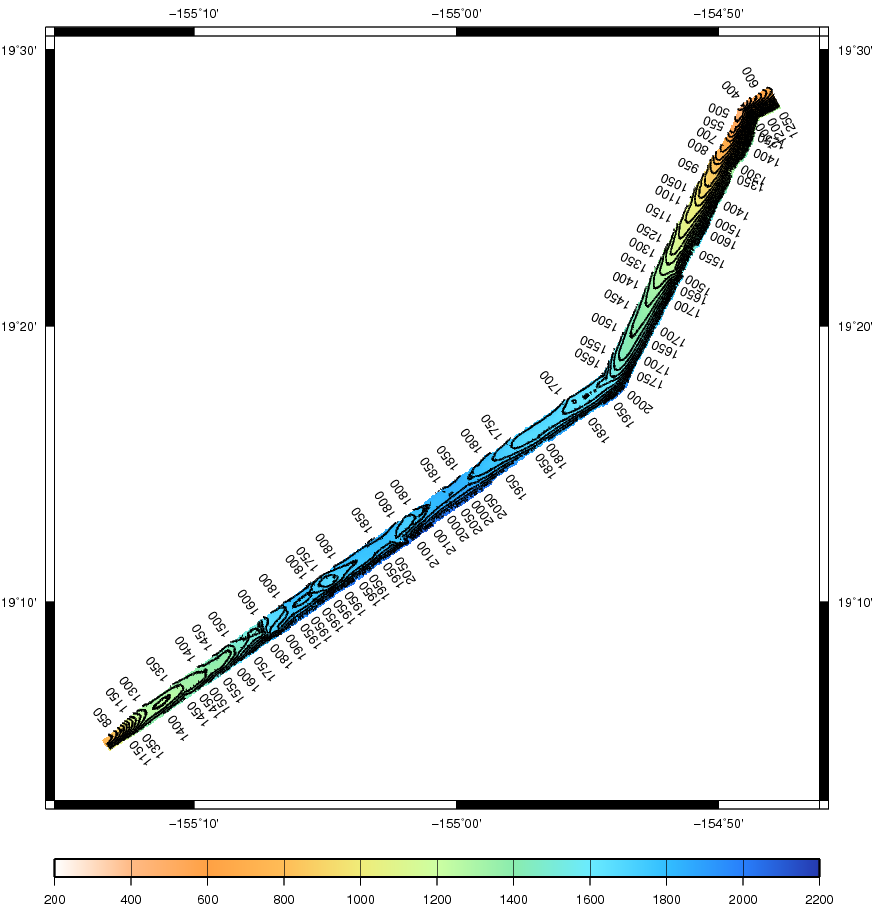
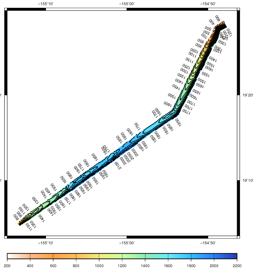
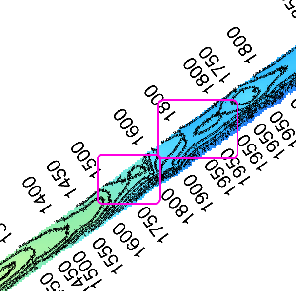
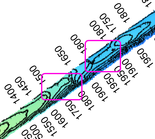
The measured means square error (MSE) for the two datasets is of about 2 meters per beam: This result by itself is not bad (considering the bathimetry extends to 2000 meters) and it is probably smaller than the sonar tolerance range, but error peaks as the ones that seem present by looking at the contours in the previous images may be unacceptable. This needs to be investigated further.