Final - It's All About Me
For this year's final we were supposed to analyze Andy's electric, water and gas bills over a period of
about 10 years, to extract short and long time trends. Also, we were challenged to identify
some interesting events (the installation of a bigger fish pond,
a couple of guest staying home for some weeks, installation of a thermostat, switching to more efficient
light bulbs and so on)
Used Software
For data analysis I decided to use SciLab. SciLab is a free clone of Matlab, and, among other
things, allows to perform data analysis and 2D / 3D ploting 2D or 3D using a simple scripting language.
Plotting Raw Data
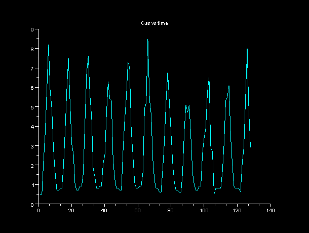
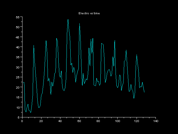
The three following plots show the variations of gas, electricity and water bills over time. The X-Axis unit is
months, starting from august 1998 to march 2009 (128 months). The seasonal variations in Gas and electricity due
to heating / cooling are extremely evident.
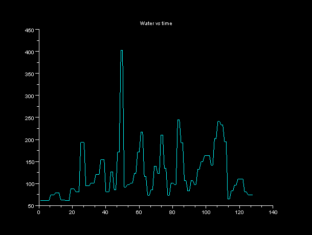
The water data shows peaks with at rough 12-month intervals. These peaks start in 2000 (the year the pond has been
installed), so they seem to be almost completely related to pond water changes in the summer (garden watering too?).
Extracting Seasonal Trends
The first data analysis step I wanted to perform was seasonal trend extraction. gas and electricticy usages are deeply
dependent on heating and cooling. Therefore, I expected temperature to have a noticeable impact on those two values.
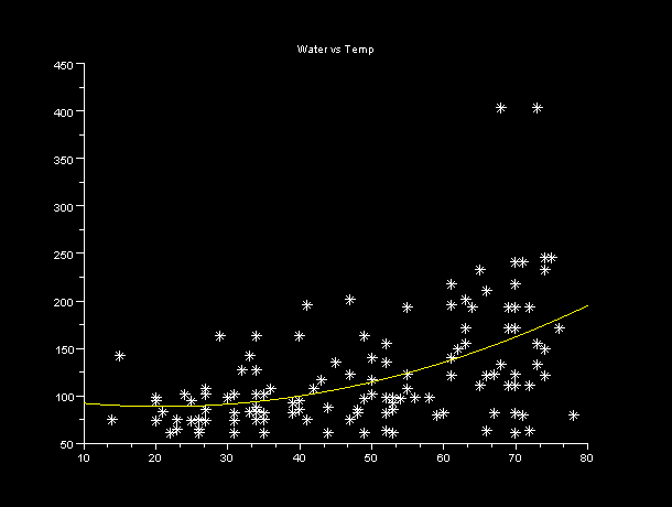
This was confirmed by representing gas and electricity costs against temperature as scatter plots:
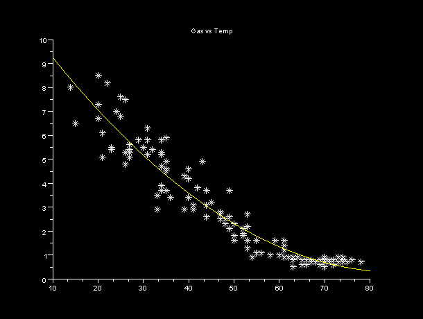
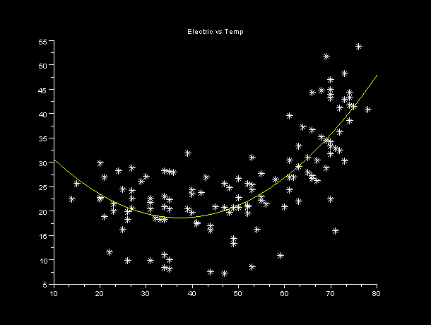
I performed curve-fitting on the scatter plots, using a second order function (the shape of data suggested second order
fitting was enough, performing third order fitting confirmed this since the third order coefficient was extremely close to zero).
Curve fitting allowed me to obtain functions that correlated temperature to the expected gas and electricity costs. It
was easy to change the domain of those functions from temperature to time (We had information about temperature for
each year/month in the dataset).
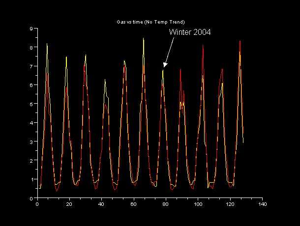
The time plot of Gas bills plus the plot of the expected cost value show how the two values closely match. This is
indicative of the fact that the great majority of gas consumption is related to heating. Also, heating appeared to
cost more than expected, until winter 2004. This is suggesting that, starting from 2005, a thermostat has been installed.
We can look for a confirmation of this by looking at electricity data:
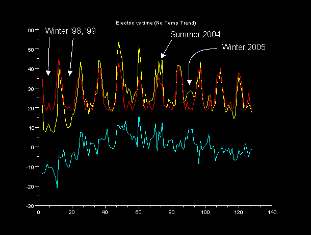
The last over-usage of electricity is evident in summer 2004, confirming the suspects of a thermostat installed in 2005.
It is also interesting to notice how electricity usage was significantly low in winters '98 and '99. Maybe no space
heater was installed at the time?
Trying to extract other events from this data proved to be almost impossible. I tried for example to identify the
point in time when the light bulbs were changed to fluorescents: I knew that about 20 bubls have been changed
almost simultaneously. I used the following table:
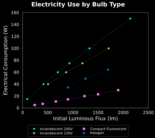
And assumed 60W bulbs were involved in the substitution. This means that
(assuming
arbitrarily lights were on for about 3 hours/day):
- Consumption with incandescent bulbs: 60W * 20 * 3h = 3600kWh/Day
- Consumption with fluorescent bulbs: 16W * 20 * 3h = 960kWh/Day
- Consumption Drop: 2640kWh/Fay
I then looked at the data (with temperature trend removed) to find consumption drops close to that value, finding
about 10 of them. I'm not even confident the light change is actually one of those points, since too many factors
are influencing data, and the calculated drop due to light substitution is a rough approximation anyways.
Water data
Season trends in water data were much less evident, but it was still possible to extract a temperature-related trend.
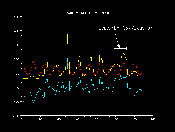
Comparing water consumption with temperature-based trends evidences an interesting over-usage period that goes
approximately from september 2006 to august 2007. I was not able to map this to one of the 'events' suggested
by Andy.
 Share this Page