Transient Throttle Conditions and How to Set it up on Modular ECUs

This is the middle part of my fuel model talk from PRI in 2016, but I’ll also be discussing settings in the Modular ECU specifically in this article.
Firstly let’s discuss what happens in a transient throttle condition – specifically when you open the throttle. We have all driven cars with aftermarket ECUs with no consideration for what happens in a throttle transient condition and we know they feel awful, but to properly understand what needs to be done, we need to understand the physics of what’s actually happening in the engine and why we need to consider transient conditions in the first place.
The other consideration, once we know what happens in the engine, is what do we do about it. I’ve seen some other ECUs with up to 8 different tables to make different changes to the amount of fuel injected under transient throttle conditions, and often it’s not clear which one needs to be adjusted. They all interact and as I said in the talk about the steady state fuel model, if you need 8 separate tables with values that don’t relate to what the engine is doing, or that aren’t replicated across engines, then perhaps the model isn’t reflecting the engine very well.
There are 3 reasons that we need to deal with transient conditions on a port injected engine.
The first reason is that measuring MAP is hard. The manifold pressure changes throughout the engine cycle due to each cylinder or rotor doing its induction stroke. Here’s a picture taken from an inline 6 cylinder engine.
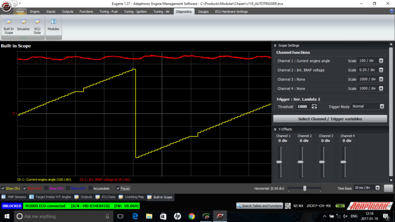
Unfiltered IMAP
To get this signal smooth enough to be useful, this must either be filtered in the time domain or the angle domain, otherwise even at idle the MAP signal will jump around and so will your fuel delivery. One way you can do this is with a simple time based filter, which introduces a delay. Another way is with an average over an angle interval, in this case 120 degrees. A third way, which we don’t do but I’ve heard other people suggest, is to just take the MAP signal at a single angle so it’s at the same point in the wave each time. Both the angle-based methods introduce their own delays, in that the signal you are looking at could be up to 120 degrees old. At low engine speeds, for example idle, this could correspond to enough time for a throttle to open and air to rush into a cylinder that’s currently doing an induction stroke. So we need some way to estimate what the ACTUAL manifold pressure is, at least well enough to handle the transient condition.
A second problem is the fuel film or wall-wetting situation. Unfortunately on a port injected engine, when the injector delivers a certain amount of fuel, not all of it goes directly into the cylinder or rotor. A certain percentage ends up on the runner walls on a film (or “pool” or “puddle” if you like). This fuel isn’t wasted; it evaporates over time and gets drawn into the engine as fuel vapour. However it doesn’t go into the cylinder immediately; it has to form a film first which then evaporates over time. As the delivered fuel quantity changes with different loads, the steady state size of the fuel film also changes. Therefore if the ECU just starts to deliver the correct new fuel quantity, then a large portion of this fuel delivered will be taken up by “filling up” the film to its new steady state value. This is the key reason for needing what is often called “acceleration enrichment”. It’s not actually enrichment the engine needs; but the ECU needs to inject more fuel, just to get to the same air-fuel ratio, because of this fuel film effect.
The final problem is what I’m going to call the “gulp of air” problem. In many situations, the fuel is injected before the inlet valve is opened because of how the injection timing is set. On a 4 cylinder engine, one cylinder will always be doing an induction stroke whenever you open the throttle, which means that one cylinder is always going to have inadequate fuel delivered if it was delivered before the throttle was opened – the ECU would need a crystal ball to be able to predict when you were going to open the throttle, at least on a mechanical throttle system. So the ECU needs a way of delivering an additional squirt of fuel to chase down the air, and this is called an asynchronous injection pulse. It’s asynchronous because it happens out of the sequence of the regular fuel injection pulses, which are timed with the engine rotation.
Let’s first talk about the first problem, which is the filtering required on the MAP signal slowing it to the point where it becomes a problem for transient throttle conditions. I don’t know how other ECU manufacturers get around this problem, other than the method I described before of having 8 different tables for the amount of fuel enrichment to provide based on certain throttle opening percentages and rates. The reason we don’t want to do that is firstly we used to do that, and it was fiddly to set up and didn’t give very good results. Secondly, it’s not a very good model of the system. If you imagine an engine at idle, the MAP might be about 30 kPa. If you suddenly open the throttle all the way, the MAP will jump up to 100 kPa as quickly as you can move the pedal. However if the MAP sensor has not responded appreciably due to the filtering, then you would need a 200% enrichment to deal with this situation. If you’re needing 200% enrichment to reach the correct value, it means you’re starting with the wrong value in the first place. And lastly, if someone had to change their MAP filtering because of some unstable reading on boost or whatever, it would change what you’d need to enter in the acceleration enrichment settings, when nothing on the engine has changed.
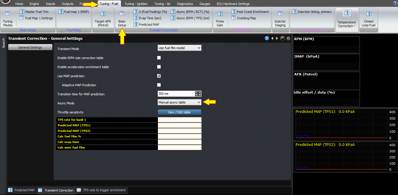
The way we do it instead is we have a model of the engine’s MAP at different RPM and TPS combinations. The Predicted MAP table is visible under the fuel tuning, transient corrections section, and this is a table of the actual MAP value that you would get under each RPM / TPS combination. On a dyno it’s very easy to fill out manually, and there’s an adaptive MAP prediction setting where the ECU will learn the predicted MAP value as you reach each condition. When the ECU detects a rapid throttle opening, it looks at the greater of either the predicted MAP, or the measured MAP from the sensor, for a fixed amount of time called the “transition time for MAP prediction” under the basic setup. You can also disable MAP prediction entirely on this page if you want to.
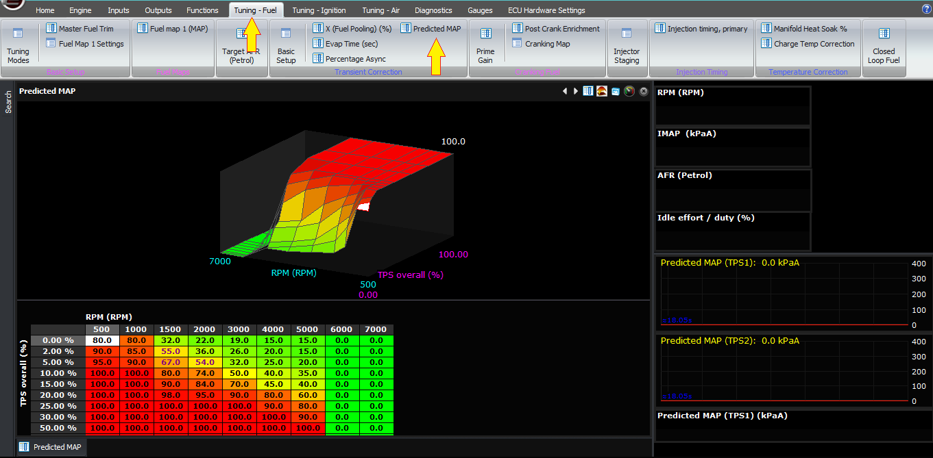
Tuning Fuel>Predicted MAP
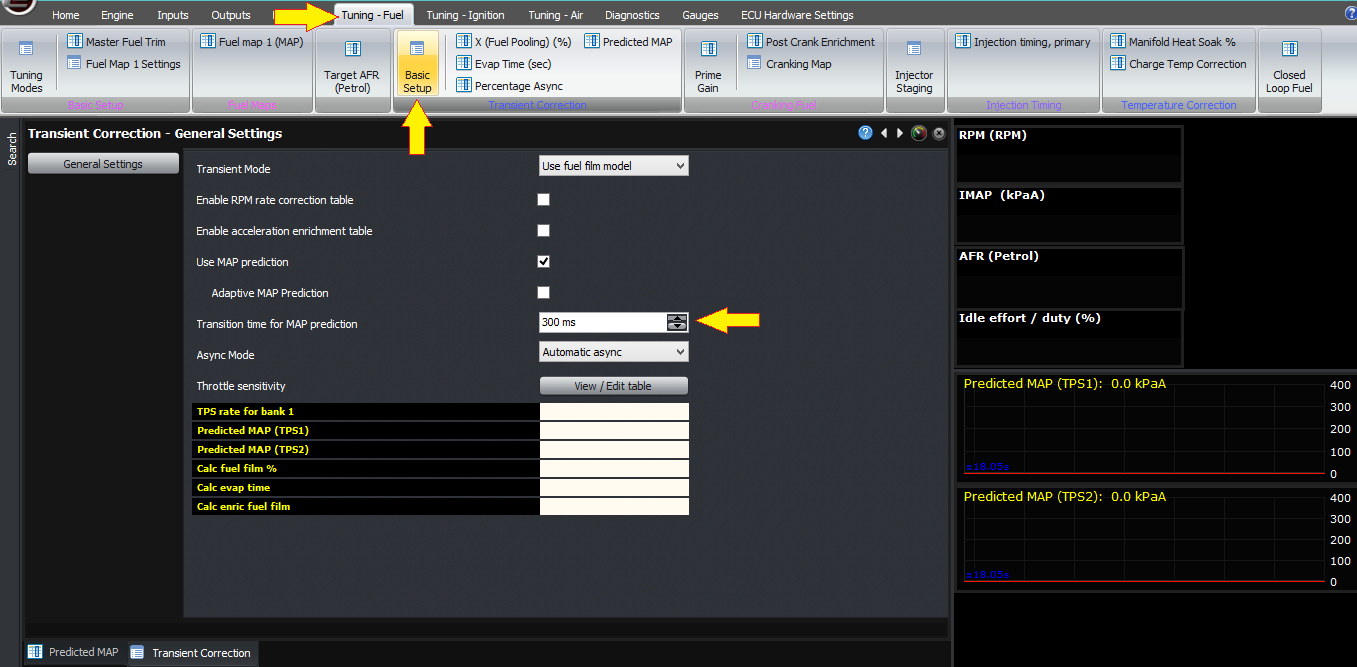
Tuning fuel>BasicSetup>Transition time for MAP prediction
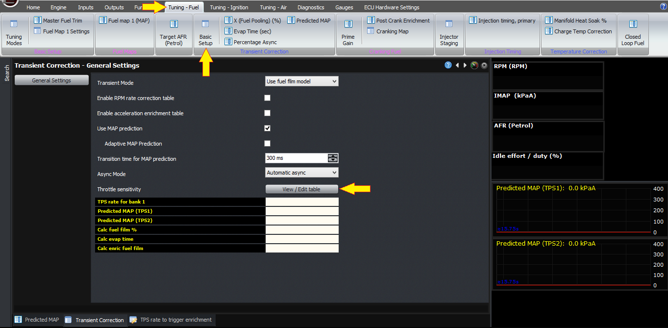
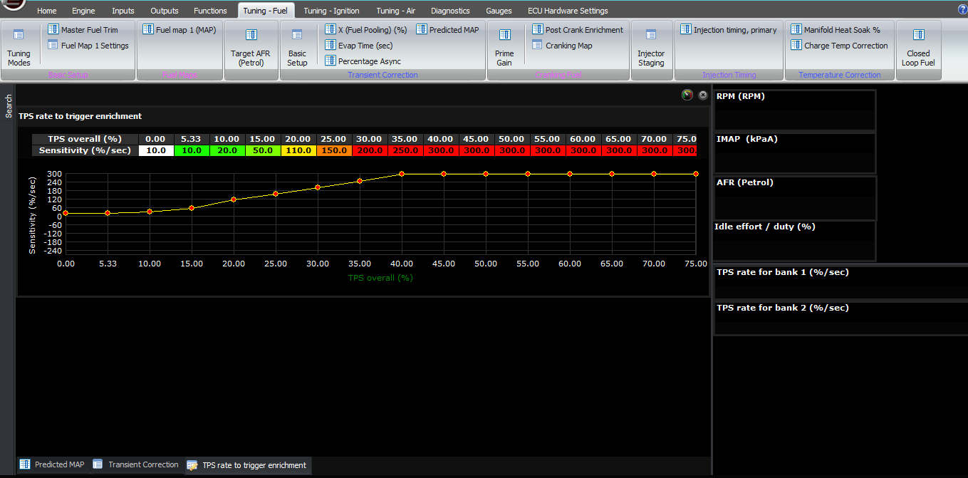
The other setting relevant to the MAP prediction is the throttle sensitivity, which is how fast the throttle has to be opened, to trigger MAP prediction. If you click on the button for the throttle sensitivity table, you can see the threshold rates (in %/second) required to trigger the MAP prediction at each TPS opening point, and the live view at the bottom tells you the current TPS rate. So you can play with the pedal yourself and visualise what numbers you get with different rates of pumping the throttle, if the numbers themselves aren’t clear.
Once you’ve entered the MAP values at each RPM / TPS combination, you can check that it’s working correctly under different conditions by either logging or using a live log view of the IMAP or intake manifold absolute pressure. When you do a throttle transition, you should see a step change in the IMAP because of the MAP prediction and it should transition pretty smoothly to the steady state value from the MAP sensor. If it’s very slow to rise then either the predicted MAP value is too low, or the throttle sensitivity is too high so it’s not triggering the MAP prediction. If it jumps high and then comes back down with a step when the MAP prediction time is over, then that means your predicted MAP value is too high for that RPM / TPS combination.
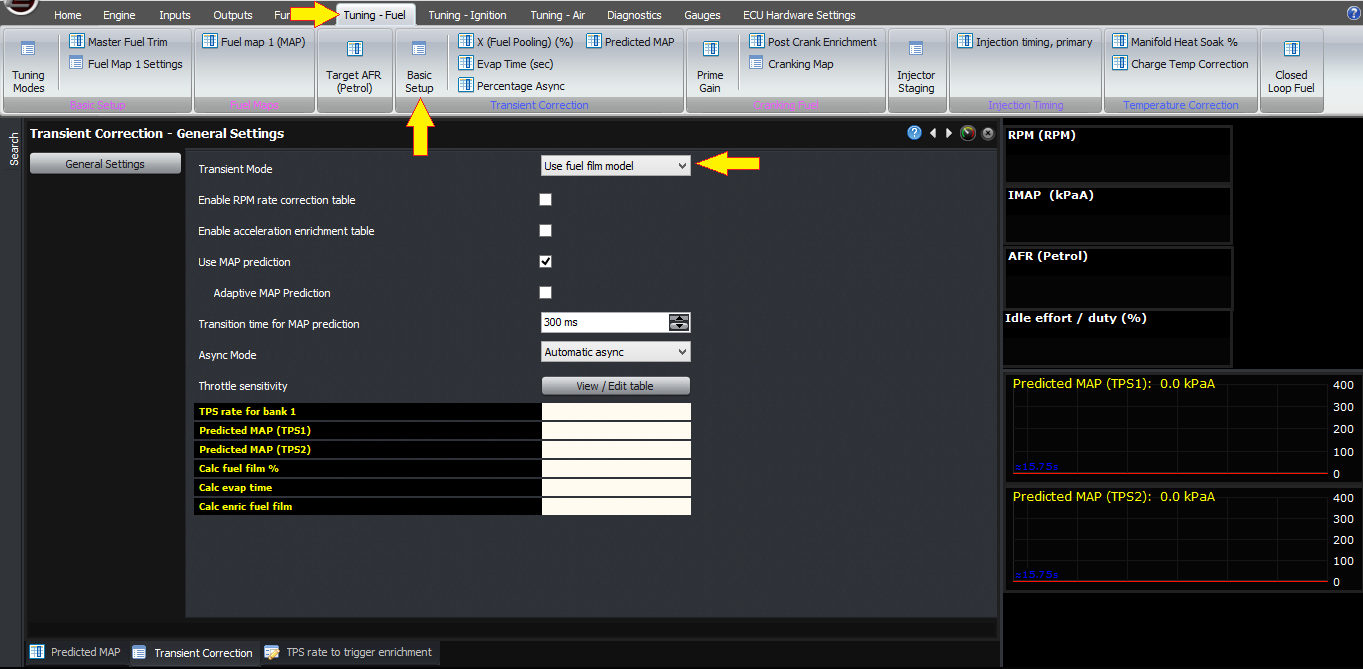
Enabling Fuel Film Model
Now let’s talk about the fuel film phenomenon. This is the way we prefer to handle transients, and the way to enable it is in the transient throttle basic setup, to select the transient mode as “use fuel film model”. The theory of this was explained in a youtube video by an ex-Ford engineer Dr Jim Cowart (https://www.youtube.com/watch?v=0ItkpVofKLw), and he describe the “X-Tau” model, where X is the percentage of fuel that ends up on the runner walls in a flim, and Tau is the time constant for it to evaporate. He describes that X is mostly dependent on coolant temperature and to a lesser extent manifold pressure, whereas Tau is mostly dependent on RPM and to a lesser extent, manifold pressure. In our software we call it “fuel pooling” and “evaporation time” to make it a bit more easy to understand and remember.
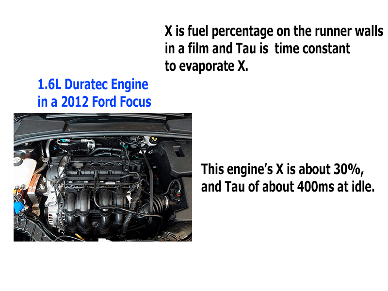
Dr Cowart mentioned in his video that the Ford Duratec engines he was calibrating had X of about 30%, and Tau of about 400ms at idle. I’ve found with most Japanese engines that X is only about 15% with standard injectors – although if you have a narrow spray pattern injector like an Injector Dynamics one, and a dual inlet valve head, then often the injector stream points right at the divider wall between the two runners, and a lot of fuel ends up on the divider. This has the effect of increasing X; so an engine that might be 15% on factory injectors might increase to 40% or so with upgraded injectors.
If we take Dr Cowart’s example, let’s further assume the engine requires 10mg of fuel per induction stroke at idle, and 40mg at WOT.
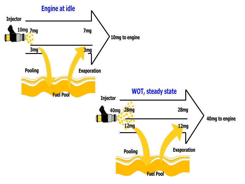
If X = 30%, that means that out of the 10mg injected, 3mg goes into filling up the film, and 3mg worth of film evaporates and gets sucked into the engine, in the steady state. The fuel film remains the same size, and 10mg still gets injected into the engine.
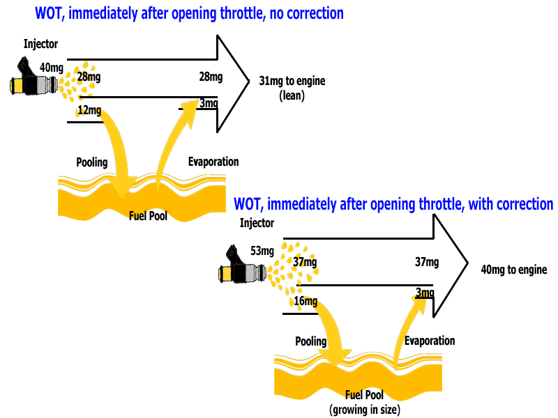
We open the throttle to wide open from idle. We know that we need 40mg to go into the engine, but if the ECU delivers 40mg, then only 70% of that, or 28mg goes straight into the engine. The other 30% or 12mg goes into the fuel film, and 3mg evaporates from how big the fuel film was before. So the engine gets 31 mg of fuel instead of 40.
So instead the ECU calculates that the engine needs 40 mg of fuel. It knows, based on the model of the fuel film, that it has enough fuel film to deliver 3mg of fuel. Therefore it needs to inject enough fuel the 70% that will go into the cylinder will equate to 37mg. This means the ECU needs to inject 37 / 0.7 = 53mg – and the other 16mg will go into building up the fuel film on the runner wall.
Another way to think of this is an “enrichment” of 32%.
This technique, according to Dr Cowart and also our own testing, works really well for hot engines, cold engines, different throttle opening rates, vacuum boost, engine size, injector type and all the other things that are built into the model.
In terms of the values for X and Tau settings, I watched the video and waited for the punchline which was how to determine what X and Tau should be… and unfortunately they need to be determined empirically. Ie, they need to be tuned. Sorry!
For this to work, firstly disable the asynchronous injection because that will complicate things. Secondly try to set the injection timing so that the throttle response is best (even though it won’t be great).
Disabling Async
X is the amount of fuel that ends up on the runner walls. So if you increase this, it will increase the additional amount of fuel the ECU will inject. So if it’s lean when you first open the throttle (eg for 200ms or so), then increase X.
If it goes rich and then lean, then that probably means that X is too high but the time is too short. If it goes correct, but then lean, then X is probably about right but the time is too short. If it’s correct and then it goes overly rich, then try reducing the time.
In general Tau or the evaporation time reduces with RPM. Times are normally in the region of 0.15 – 0.4 seconds at idle. I haven’t found it changes appreciably with manifold pressure.
X, or the percentage fuel pooling, varies with coolant temperature because it affects the temperature of the runner wall and therefore how much fuel condenses. As I mentioned before, a well set up engine like an OEM one in my experience requires X about 15% when hot and slightly more when cold (eg 25%), but with people putting on aftermarket injectors with spray patterns not matched to the engine, this can go up to 40% or so on even a warm engine.
The last topic we will discuss is the asynchronous injection, to deal with the “gulp of air” issue. Firstly, sometimes people say things like “well, how fast can the air really move anyway, it’s got to get all the way from the throttle body, fill up the plenum and into the cylinder”. If you have a pressure drop with a ratio of more than 2:1, which you would on most engines at idle, the air actually goes sonic through the restriction, ie at the speed of sound. The speed of sound at atmospheric pressure is about 300m/s, so to travel the distance between the throttle body and the cylinder, which unless you have a supercharged Lotus will be less than a metre, we are talking about a few milliseconds.
I explained the theory behind it before in the introduction, so let’s look at an example. Let’s choose the example before where we have an engine at idle which needs 10mg at idle, and then 53mg to be injected immediately after we open the throttle. If we’ve done a closed-valve injection, then we’ve already done the injection pulse before we knew how big it needed to be. So instead we will do an asynchronous injection pulse to make up the difference. In this case, the difference that we need to make up is 43 mg.
Whether we actually need to do this 43mg, or a slightly higher or lower amount, depends on injector timing, injector placement and other factors.
The normal way we do this is by selecting the Async mode as being “automatic async”. Then, we have an async gain map where we can adjust the amount of asynchronous injection burst, relative to coolant temperature and RPM. Often at lower temperatures, more async is required, up to 200% with E85 for example – and at higher engine speeds, less async is required.

Enabling Async
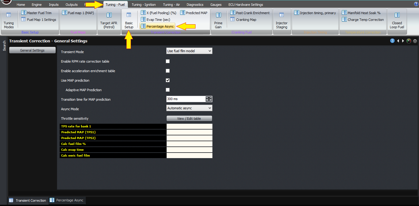
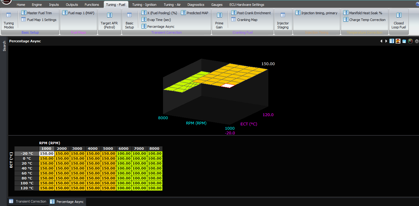
The map is called the asynchronous gain. In the above example, the ECU worked out that there was a shortfall of fuel delivered of 43mg. If you set the async gain to 100% at the current RPM and temperature, then that would cause the ECU to deliver a new pulse from the injectors that corresponds to 43mg worth of fuel. If you had set the async gain to 200%, then the ECU would inject 86mg of fuel with the async pulse. You can see that this is working on the async value in the gauges.
The best results are obtained by setting the async gain to zero, and adjusting the injection timing to optimise the response without async, optimising X and Tau and then using the async function to get the last little bit of response.
The above description should be sufficient and so far this has worked well. However if you do prefer to handle the transient conditions manually, instead of with a model, then you can also do this.
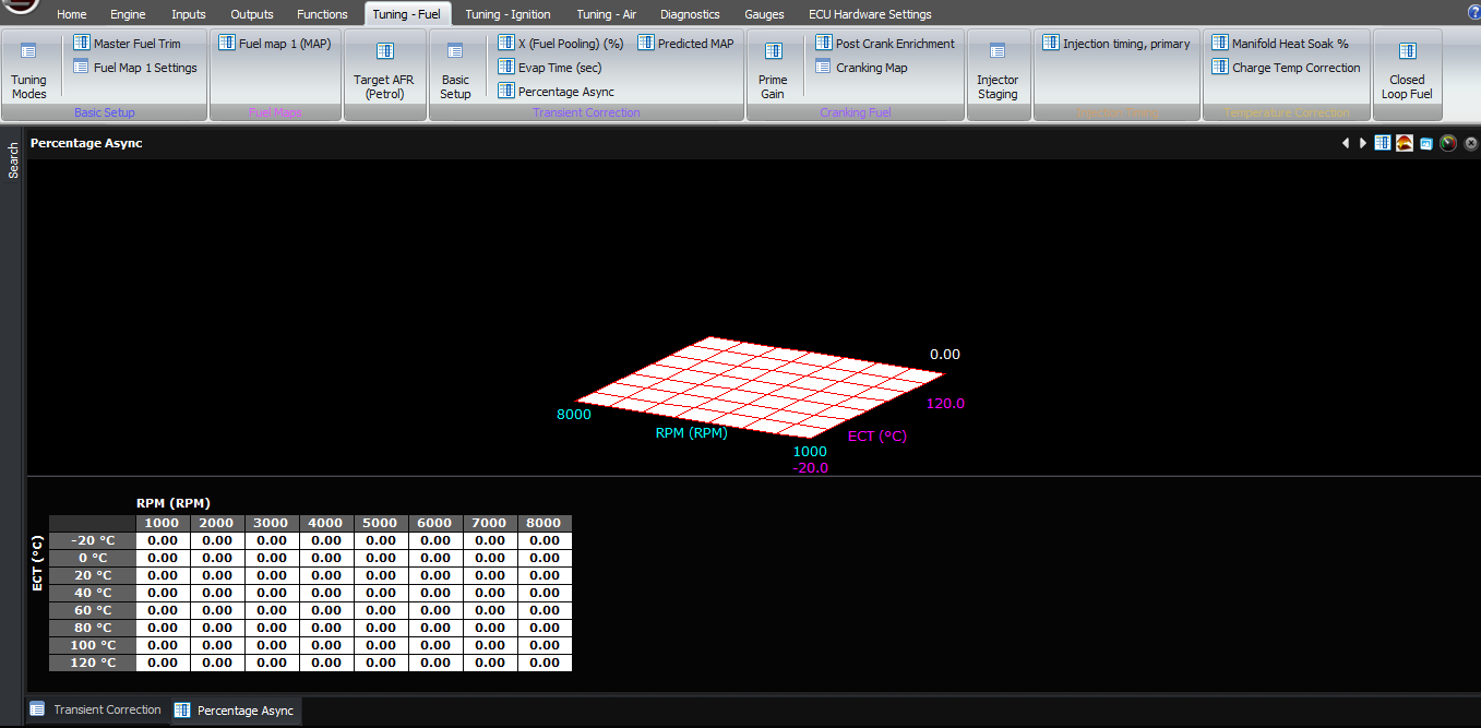
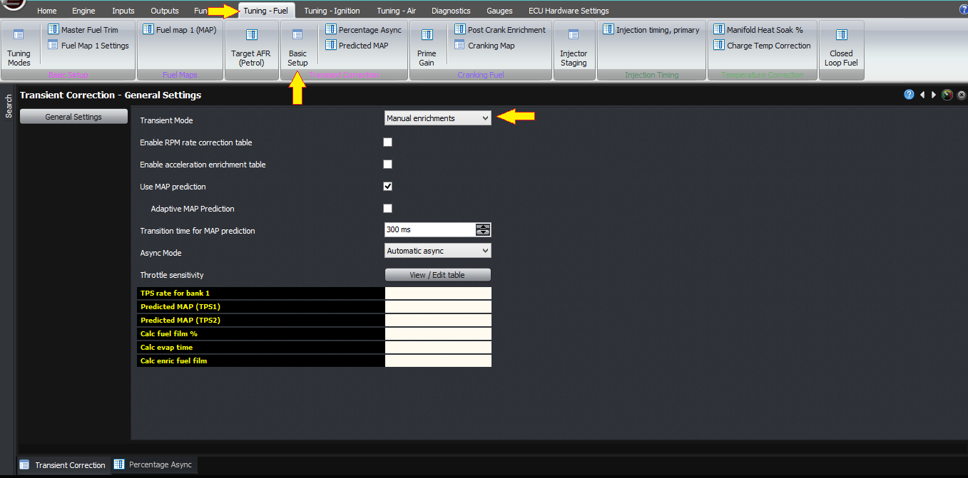
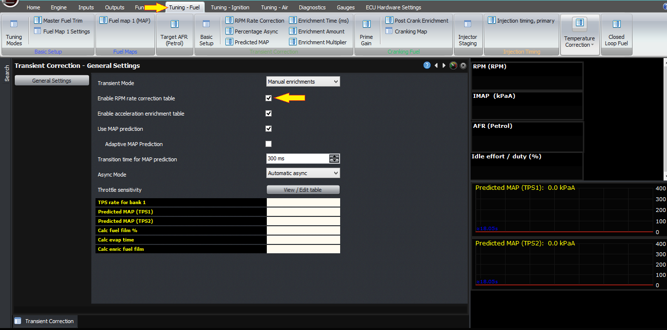
Firstly, you can set the fuel film model to “manual enrichments”, and this disables the fuel film modelling and adjustments to the fuel requirements of the engine based on transients. If you want to make corrections for transients, which you will, they will need to be done using the manual enrichment table.
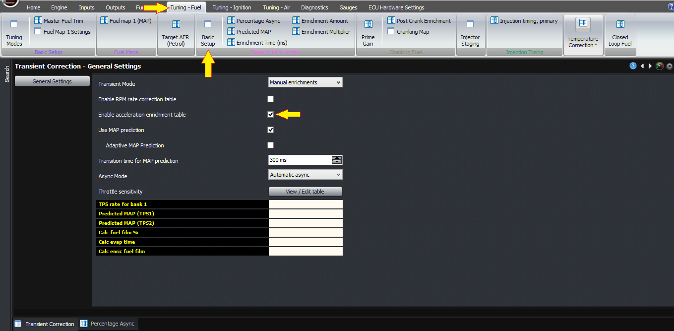
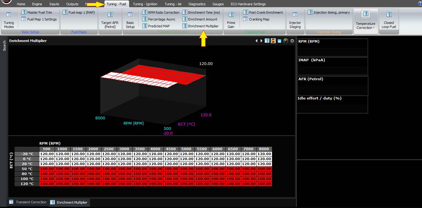
To activate the manual enrichment table, you must select the checkbox in the basic setup. This gives you three more maps; enrichment time, enrichment amount and enrichment multiplier.
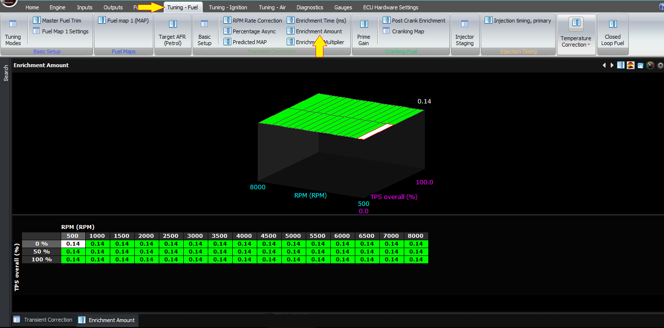
The enrichment amount is the basic table, which gives your percentage enrichment as a function of throttle position and RPM. The ECU calculates a delta of this, for example if you have 0% at TPS=0, and 40% and TPS =50%, and 50% at TPS =100%, then when you go from closed throttle to 50% throttle, you will have 40% enrichment, and then if you go from 50% to 100%, after the first enrichment has finished, you will have an additional 10%.
The enrichment multiplier table is based on engine speed and coolant temperature and allows for the fact that engines generally may need more enrichment, even as a percentage, at lower coolant temperatures. This is a multiplier, so most of the time this table should be at 100%, but if you want to add another 20% of enrichment at a certain coolant temperature, you would enter 120%.
The final setting is the enrichment time, which is another map you can adjust if you want to do it manually.
Note that you can also use this in conjunction with the fuel film model if you wish to; it just shouldn’t be necessary in theory.
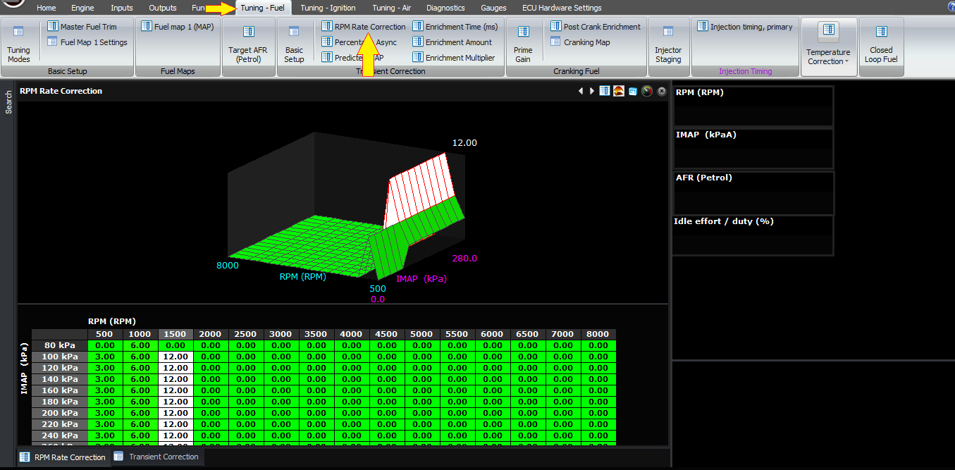
Another transient setting you can enable is the RPM rate correction table. This table is based off RPM and load, and the value is the percentage enrichment at an RPM rate of 1000 RPM/second. For example, if you wanted the ECU to always enrich by 6% for a rate of 1000 RPM/second, across all RPM and load conditions, you would fill the table with 6%. This also means that at 500 RPM/second RPM rate, you would get a 3% enrichment, and 2000 RPM/second would give you a 12% enrichment. Again this condition should in theory be handled by the fuel film model but it’s here if you want to set it manually.
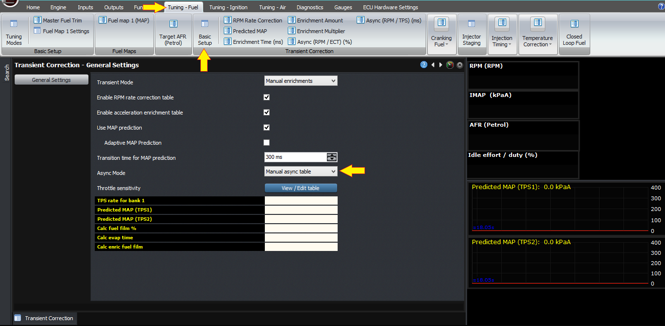
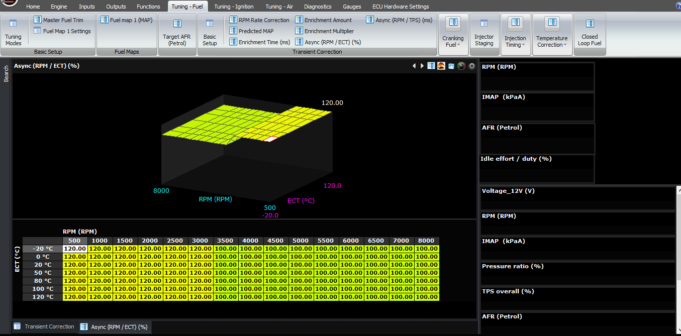
There is also a manual asynchronous mode which can be enabled, but when done so it is itself in milliseconds, not percentage or milligrams or microlitres. When this setting is enabled, you have 2 new tables; Async (RPM/ TPS) and Async (RPM / ECT). These two are multiplied together. So for example the RPM/ECT map would normally be set to 100% everywhere, except slightly higher as required at the lower coolant temperatures, and the RPM/TPS map would be your main millisecond based asynchronous pulse map.
In general we don’t recommend these manual modes, because the results are often too specific to one engine or installation, and they aren’t replicable to other engines. On the one hand it prevents us from making a good starting point because of this, and secondly it means that when people do contact our support people for help, we have no way of seeing if the table is right because it’s so specific to each engine.
Please see my other videos on steady state fuel calculation and also the injector model to gain a complete understanding of how the fuel calculations work inside the ECU.
Thank you!
©2018 Adaptronic