Principal Components Analysis

The H₂O PCA algorithm is still in development. If you have questions or comments please see our contact us document. H₂O is an open source tool and welcomes user collaboration.

Defining a PCA Model

X:

The set of numeric variables that the PCA algorithm is to be applied to. Selections are made by highlighting and selecting from the field, which populates when the data key is specified. PCA does not include categorical variables in analysis. If a variable is a factor, but has been coded as a number (for instance, color has been coded so that Green = 1, Red = 2, and Yellow = 3), users should be sure that these variables are not selected before running PCA. Including these variables can adversely impact results, because PCA will not correctly interpret them. Categorical variables that are alpha or alpha numeric will be omitted by default. These are listed under the field of X variables in a yellow message box.

Tolerance:

A tuning parameter that allows the specification of a minimum level of variance accounted for. A tolerance set at X is a threshold for exclusion so that components with less than X times the standard deviation of the strongest predictive component are not included in results. For instance, for a tolerance of 2 if the standard deviation of the strongest predictor (the first component) is .39, than any subsequent component with standard deviation less than (2)(.39) = .78 will not be included in the analysis of principal components.

Standardize:

Allows users to specify whether data should be transformed so that each column has a mean of 0 and a standard deviation of 1 prior to carrying out PCA.

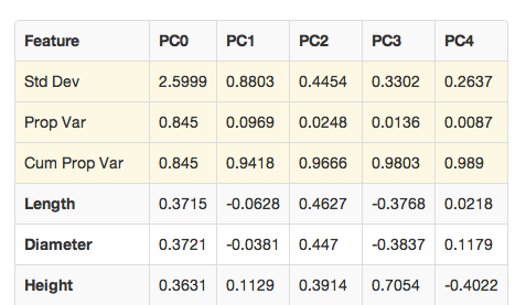
Interpreting Results

The results of PCA are presented as a table. An example of such a table is given below. In the simplest conceptual terms, PCA can be viewed as an algorithm that takes a given set of old variables, and performs transformations to yield a new set of variables. The new set of variables have useful practical application, as well as many desirable behaviors for further modeling.

Std dev

Standard deviation. This is the standard deviation of the component defined in that column. In the example shown below the standard deviation of component PC0 is given as 2.5999.

Prop Var

Proportion of variance. This value signifies the proportion of

variance in the overall data set accounted for by the component. In the example shown below the proportion of variance accounted for by PC0 is 76.5%.

Cum Prop Var

Cumulative proportion of variance. This value signifies the cumulative proportion accounted for by the set of principal components in descending order of contribution. For instance, in the example below the two strongest components are PC0 and PC1. PC0 accounts for about 76% of the variance in the dataset alone, while PC1 alone accounts for about 10% of variance. Together the two components account for 86% of variance; the value given in the Cum Prop Var field of the PC1 column.

Variable Rows

In the PCA results table the factors included in the composition of principal components are listed, and their contribution to the component is given (called factor loadings). Note that if the contributions are summed by the column, the absolute value of each of the factor loadings sum to the total variance of the principal component.

Notes on the application of PCA

H₂O’s PCA algorithm relies on a variance covariance matrix, not a correlation coefficient matrix. Covariance and correlation are related, but not equivalent. Specifically, the correlation between two variables is their normalized covariance. For this reason, it’s recommended that users standardize data before running a PCA analysis.

Additionally, modeling is driven by the simple assumption that set of derived variables can be appropriately characterized by a linear combination. PCA generates a set of new variables composed of combinations of the original variables. The variance explained by PCA is the covariance observed in the whole set of variables. If the objective of a PCA analysis is to use the new variables generated to predict an outcome of interest, that outcome must not be included in the PCA analysis. Otherwise, when the new variables are used to generate a model, the dependent variable will occur on both sides of the predictive equation.

PCA Algorithm

Let \(X\) be an \(M\times N\) matrix where

1. Each row corresponds to the set of all measurements on a particular attribute, and
2. Each column corresponds to a set of measurements from a given observation or trial

The covariance matrix \(C_{x}\) is

\(C_{x}=\frac{1}{n}XX^{T}\)

where \(n\) is the number of observations.

\(C_{x}\) is a square, symmetric \(m\times m\) matrix, the diagonal entries of which are the variances of attributes, and the off diagonal entries are covariances between attributes.

The objective of PCA is to maximize variance while minimizing covariance.

To accomplish this suppose a new matrix \(C_{y}\) with off diagonal entries of 0, and each successive dimension of Y ranked according to variance.

PCA finds an orthonormal matrix \(P\) such that \(Y=PX\) constrained by the requirement that

\(C_{y}=\frac{1}{n}YY^{T}\)

be a diagonal matrix.

The rows of \(P\) are the principal components of X.

\(C_{y}=\frac{1}{n}YY^{T}\)

\(=\frac{1}{n}(PX)(PX)^{T}\)

\(C_{y}=PC_{x}P^{T}\).

Because any symmetric matrix is diagonalized by an orthogonal matrix of its eigenvectors, solve matrix \(P\) to be a matrix where each row is an eigenvector of \(\frac{1}{n}XX^{T}=C_{x}\)

Then the principal components of \(X\) are the eigenvectors of \(C_{x}\), and the \(i^{th}\) diagonal value of \(C_{y}\) is the variance of \(X\) along \(p_{i}\).

Eigenvectors of \(C_{x}\) are found by first finding the eigenvalues \(\lambda\) of \(C_{x}\).

For each eigenvalue \(lambda\) \((C-{x}-\lambda I)x =0\) where \(x\) is the eigenvector associated with \(\lambda\).

Solve for \(x\) by Gaussian elimination.