SageMaker Canvas Demo
Marketing Response Campaign (Classification)
In this demo, we will learn how to use SageMaker Canvas to build no-code classification models to predict customers' response to marketing campaigns.
Datasets can be downloaded here:
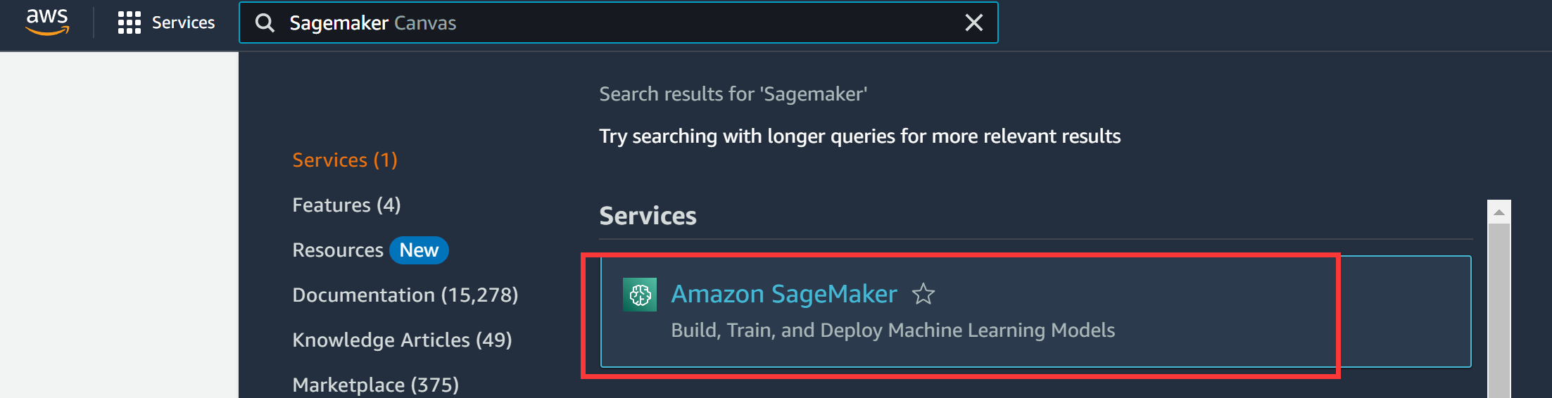
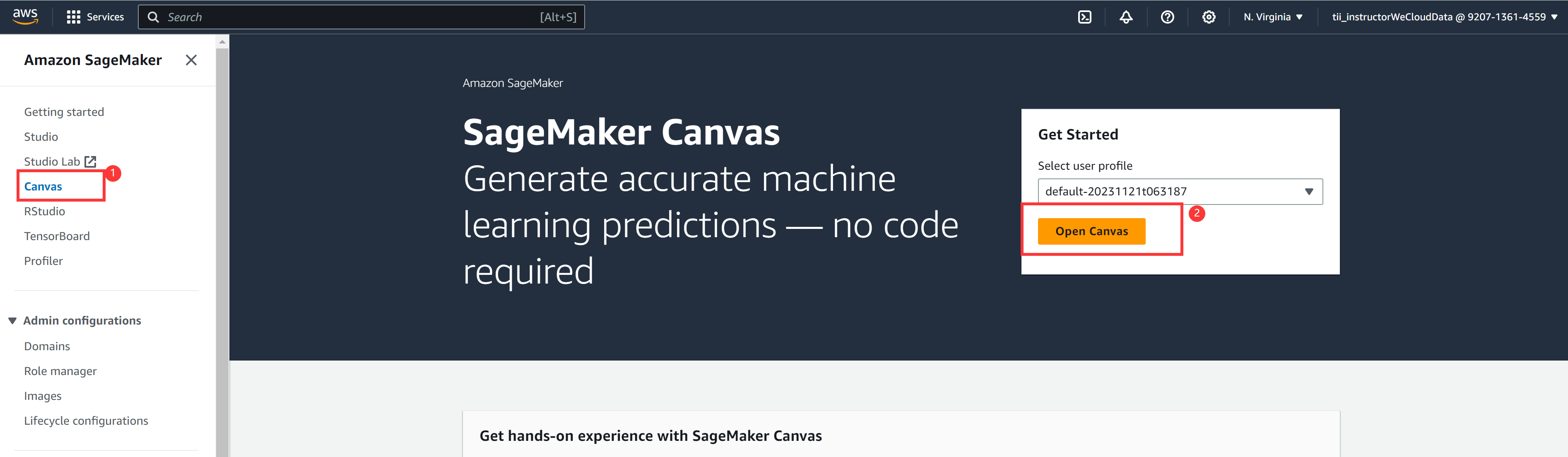
First, we need to launch the SageMaker Canvas application. For that, navigate to SageMaker service and then in the Canvas screen, select "Open Canvas":
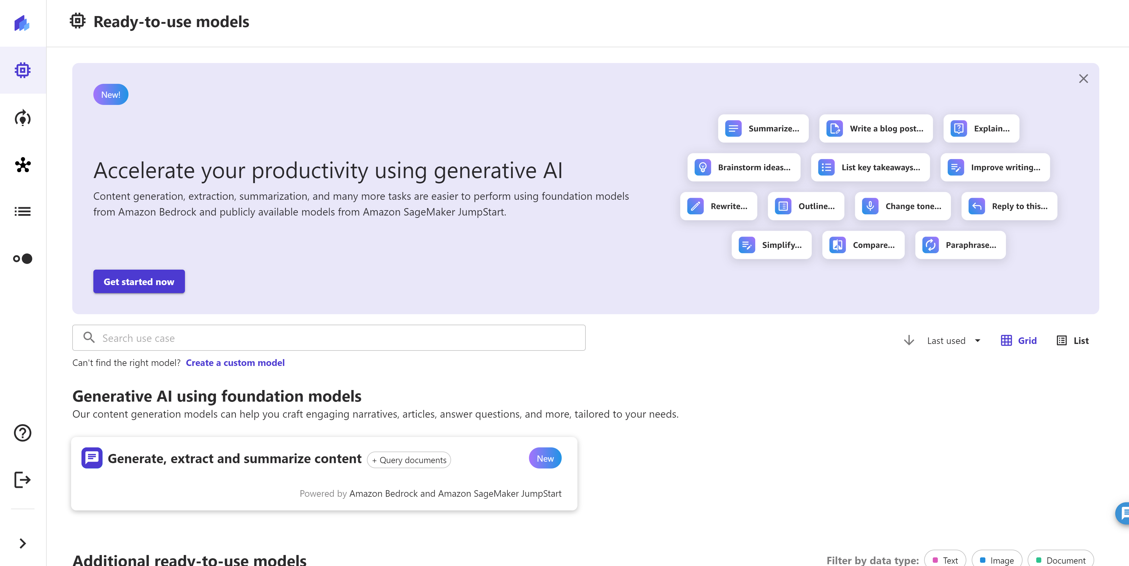
It will open the Canvas app in new tab:
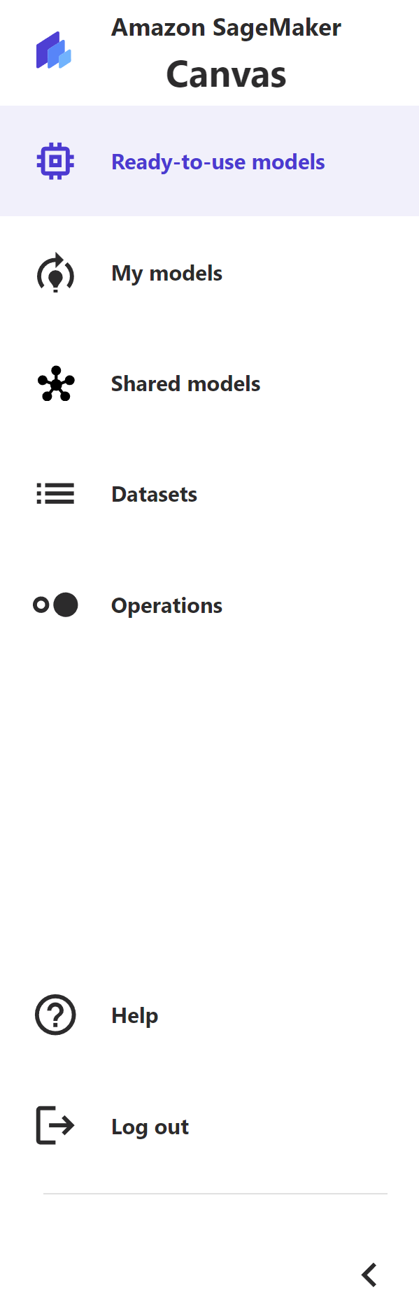
If you click on the bottom left arrow ( > ) button you can see the full name of the icons.

In this exercise, we will create a model that solve a binary classification problem. Model predicts whether a lead will convert into a sale or not based on the different marketing activities/metrics captured for that lead by the marketing campaigns. Download the web marketing data and lead data files to your local desktop/laptop. We will upload these 2 files later in the Sagemaker Canvas for training the model. Let’s have a look into the data. open both csv files in your laptop.
Download Links:
Lead Data
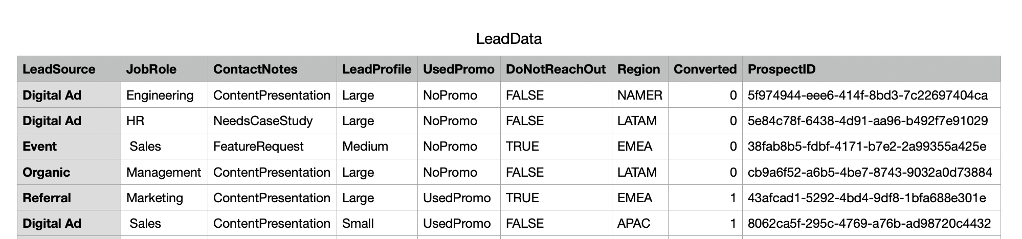
LeadData.csv file provides data about the lead and each lead has a unique ProspectID associated with it.
It provides information including job role (JobRole), lead profile (LeadProfile) , whether they used marketing promotion or not (UsedPromo), region ( Region ), unique Id ( prospectID ) and whether they converted into a sales or not ( Converted ) etc. This "converted" field is our target feature for model prediction.
Web Marketing Data
WebMarketingData.csv file provides data on what all different marketing activities / matrices were performed by the lead under different campaigns run by marketing team.
It provides data including the last campaign activity performed by the lead ( LastCampaignActivity ), number of page views per visit ( PageViewsPerVisit ), total time spend on website ( TotalTimeOnWebsite ), whether the lead attended the marketing event or not ( AttendMarketingEvent ), whether the lead viewed the advertisement or not ( ViewedAdvertisement ) etc.
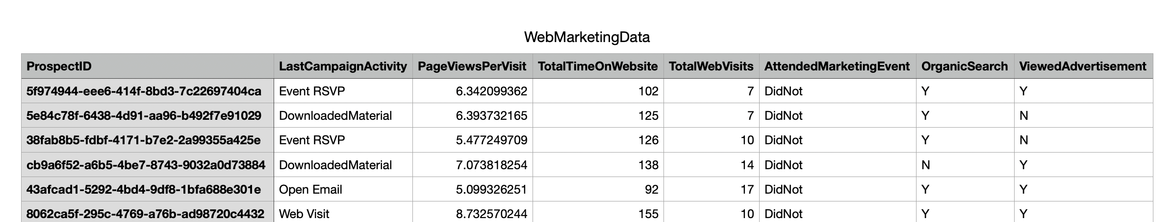
Please Note: In both files, the field "ProspectID" joins each lead in LeadData.csv file to WebMarketingData.csv file.
Now let's import both of these two files in Sagemaker Canvas to train the model.
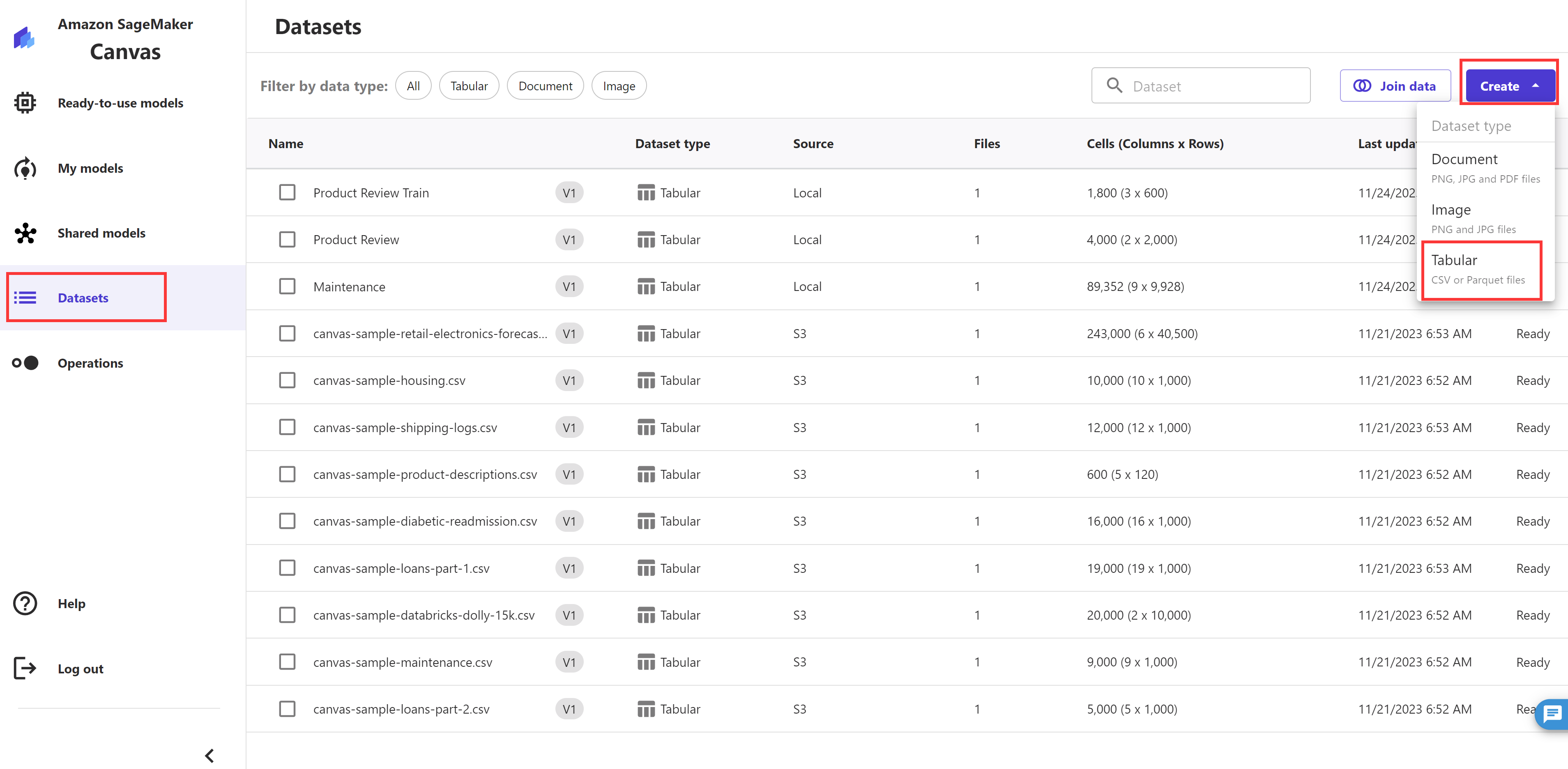
In the left panel of the Canvas console, click the Dataset, then click Create, for the dataset type, we use Tabular
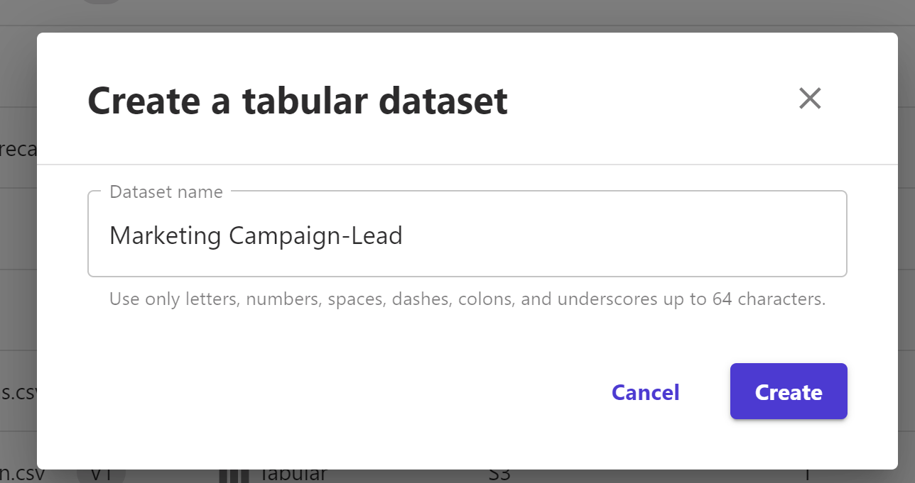
Let's give our dataset a name, for example, Marketing Campaign-Lead
For the Data Source , leave it as Local upload, click Selcet files from your computer, then select and upload our LeadData.csv. Once finished, click Preview
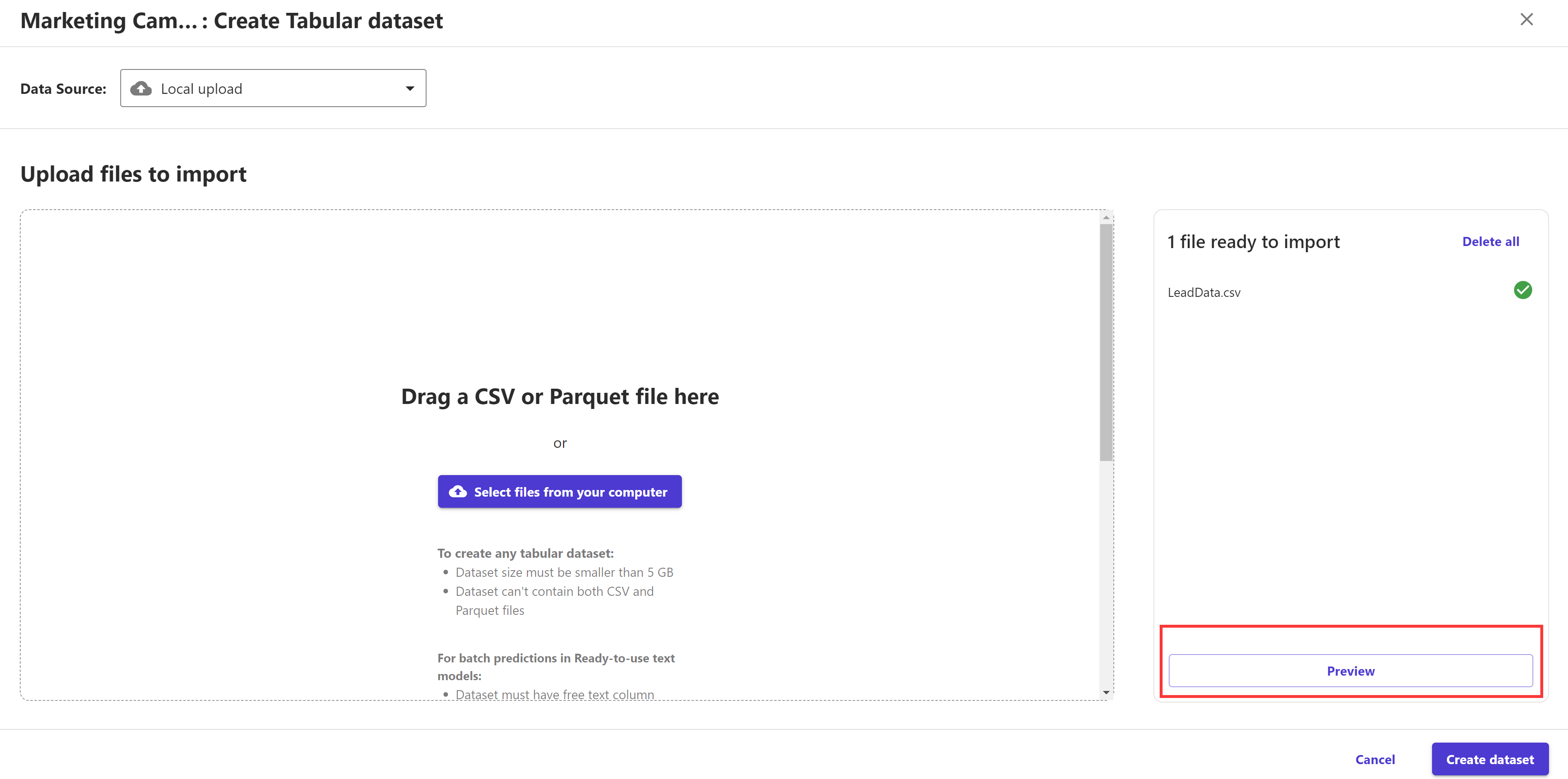
After a quick check, click Create dataset.

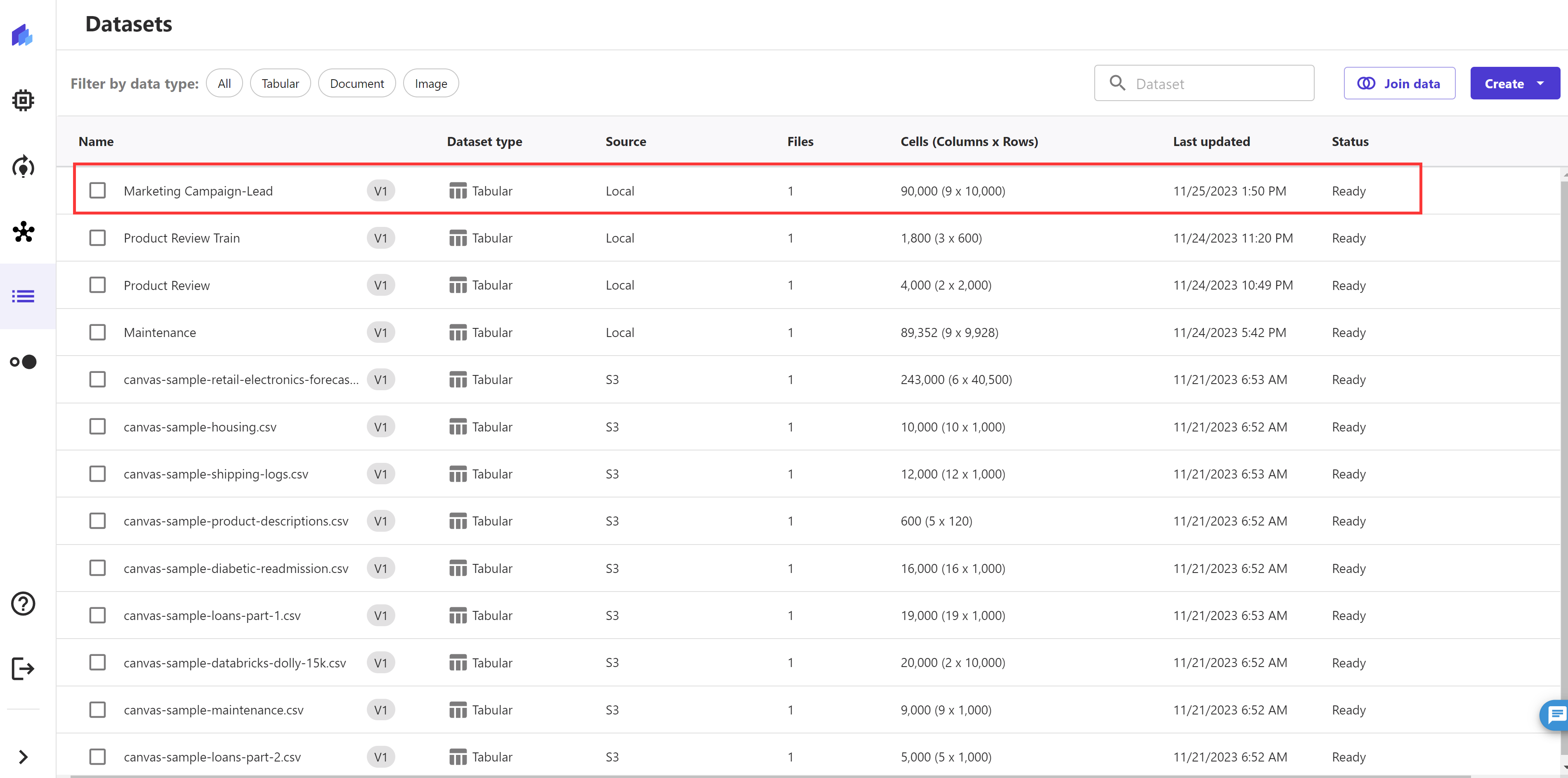
The import process takes approximately a couple of seconds. When it’s complete, we can see the dataset is in Ready status.
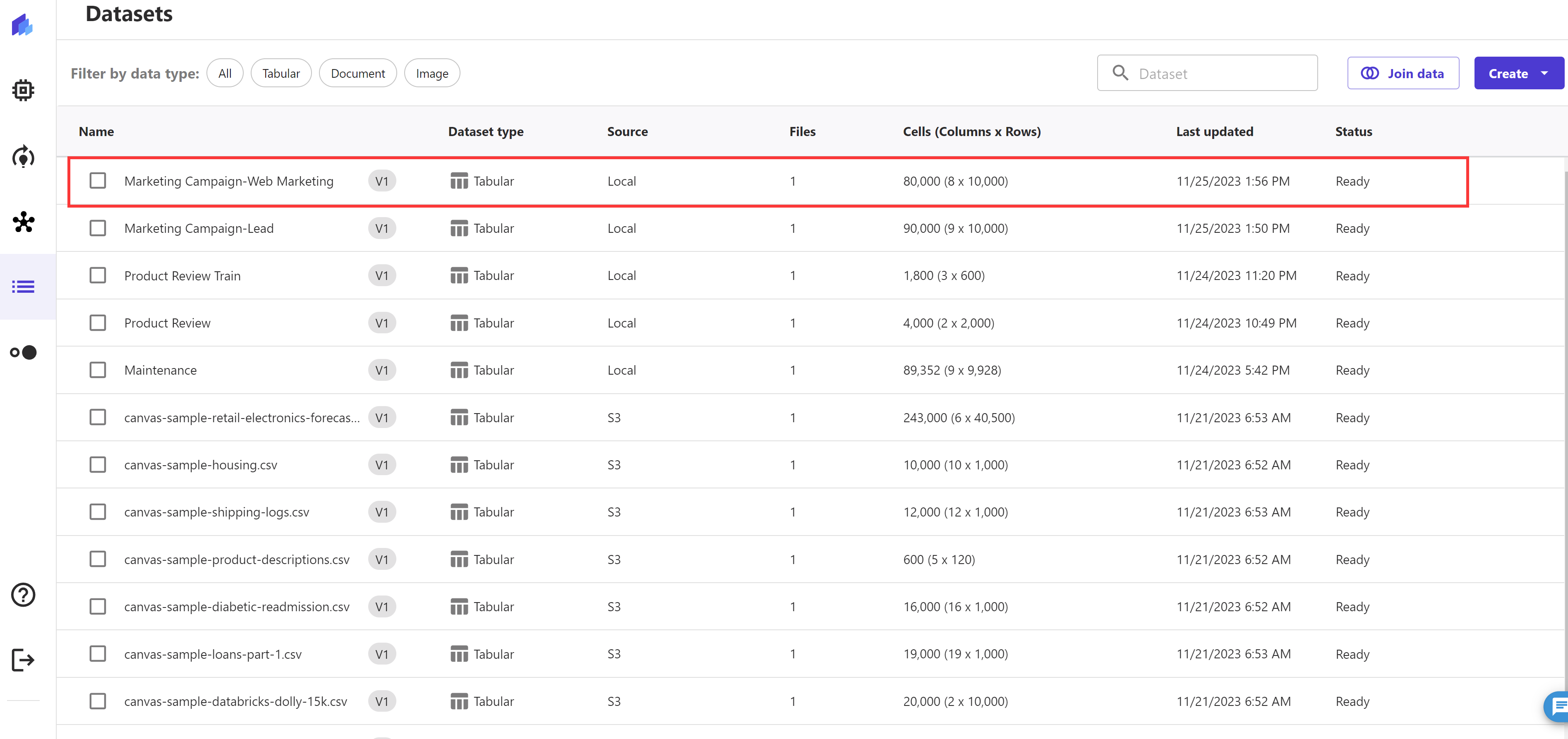
Let's repeat above steps to create the Marketing Campaign-Web Marketing Dataset from the WebMarketingData.csv file
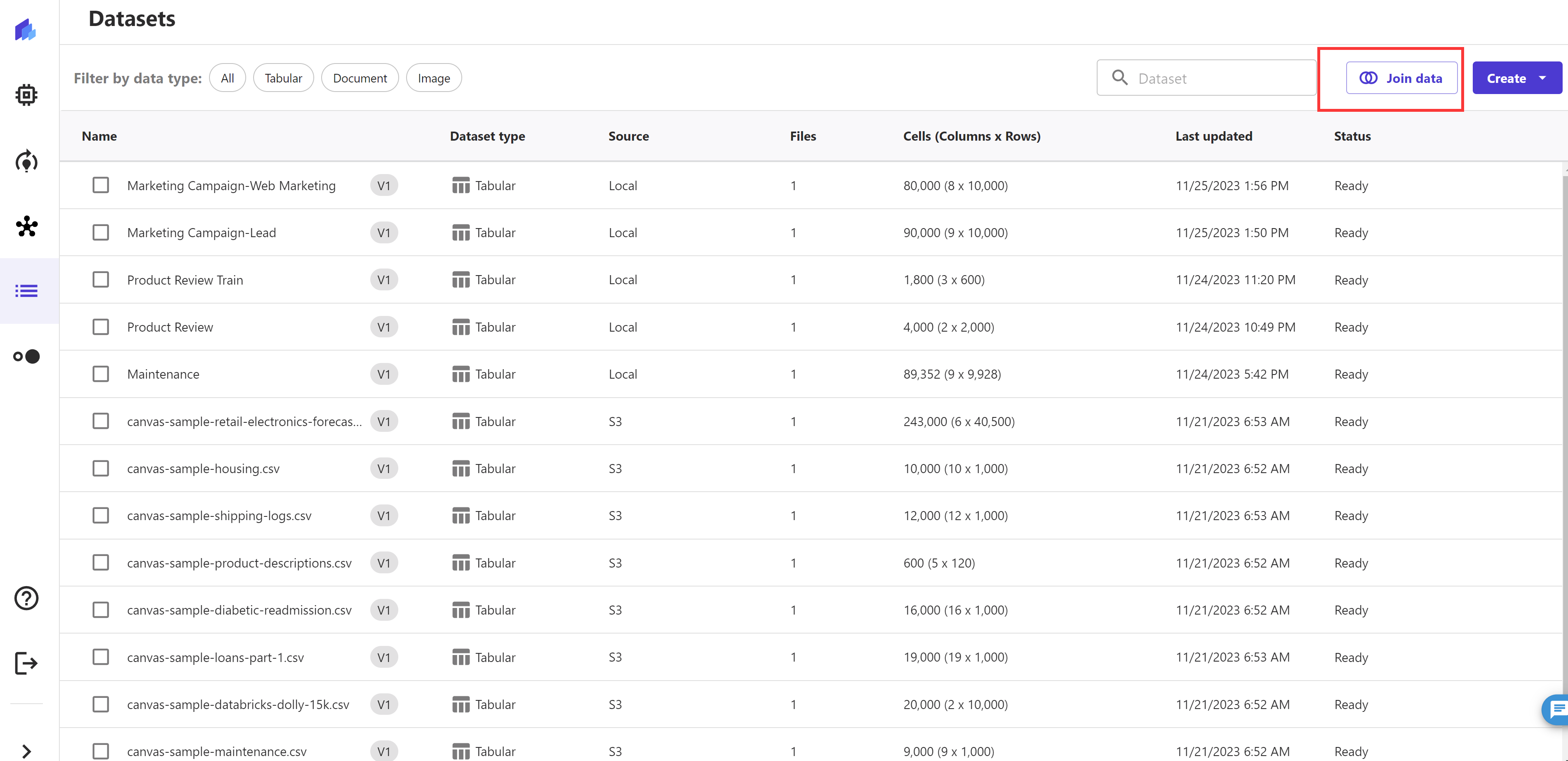
Now we can join both datasets which create a new dataset for model training .
Select the button "Join data" in the top right corner and drag and drop both of the datasets in the Canvas UI:
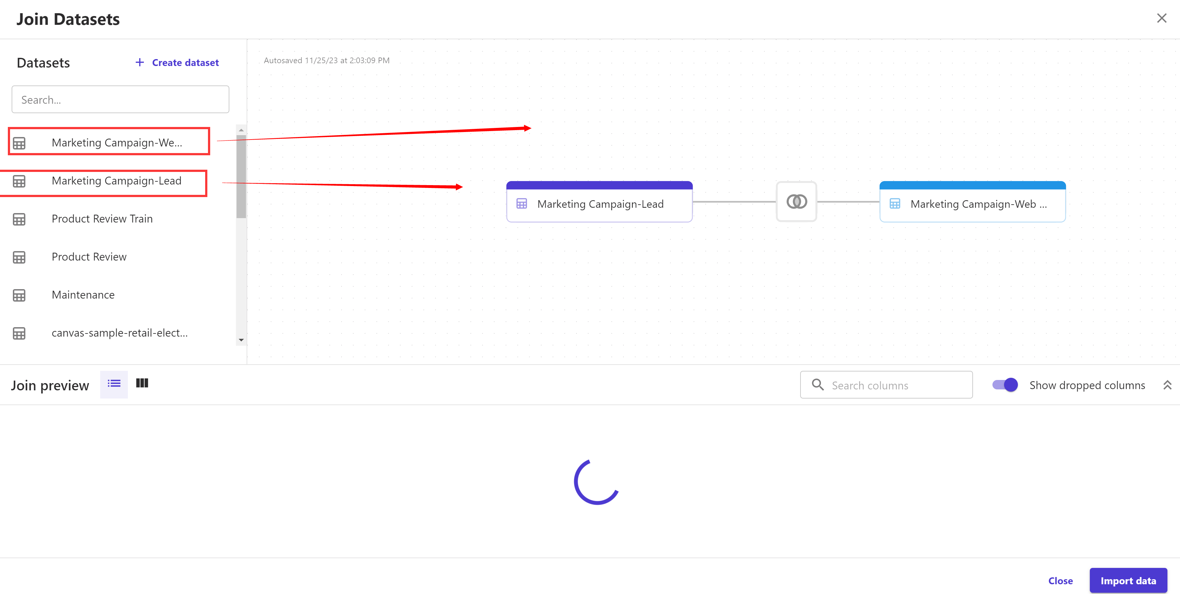
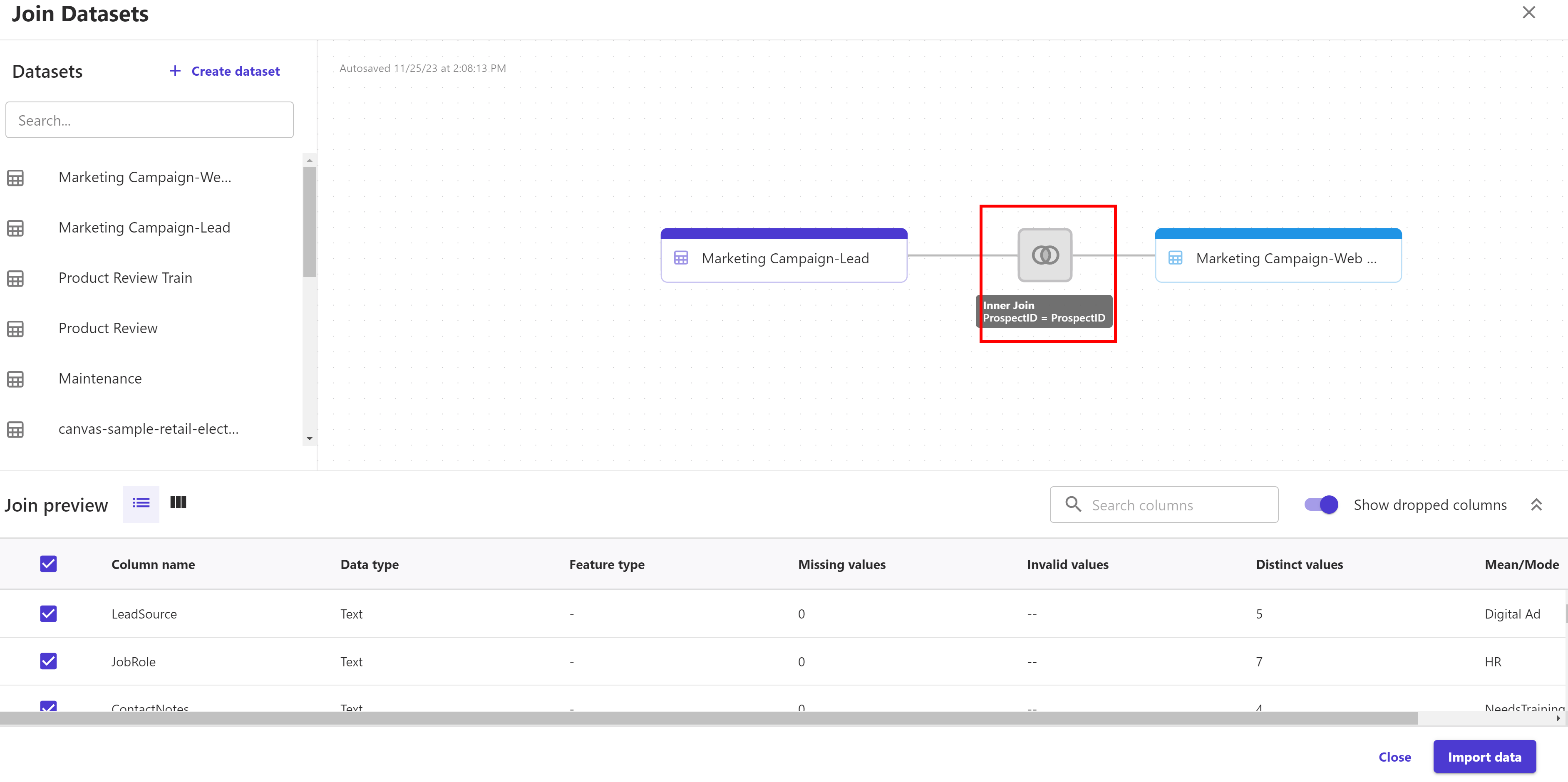
Canvas will automatically use "ProspectID" field to perform inner join for these two datasets
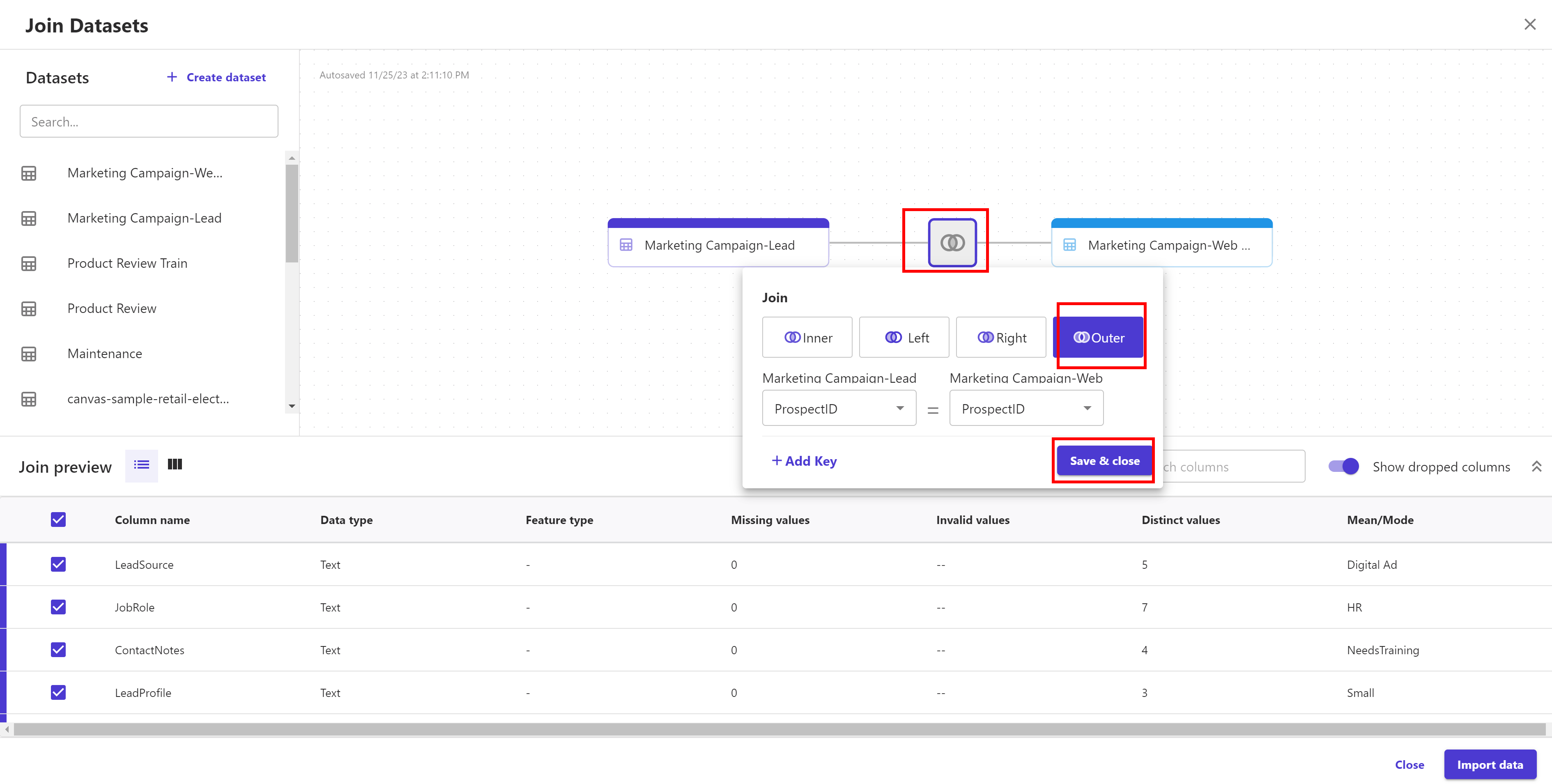
Let's switch the join method to Outer join by clicking the intersection of both the datasets. Don't forget to click "Save & Close" button
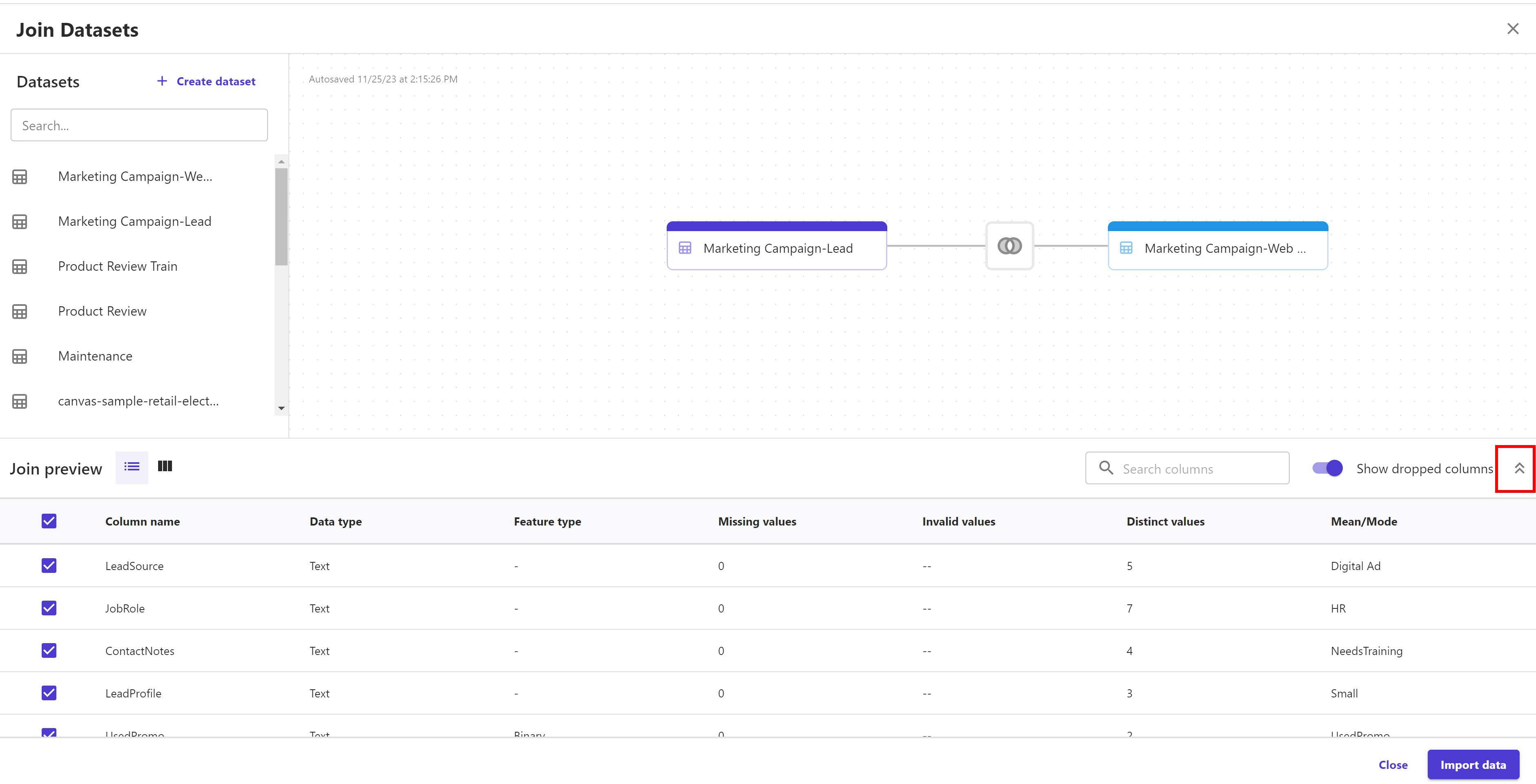
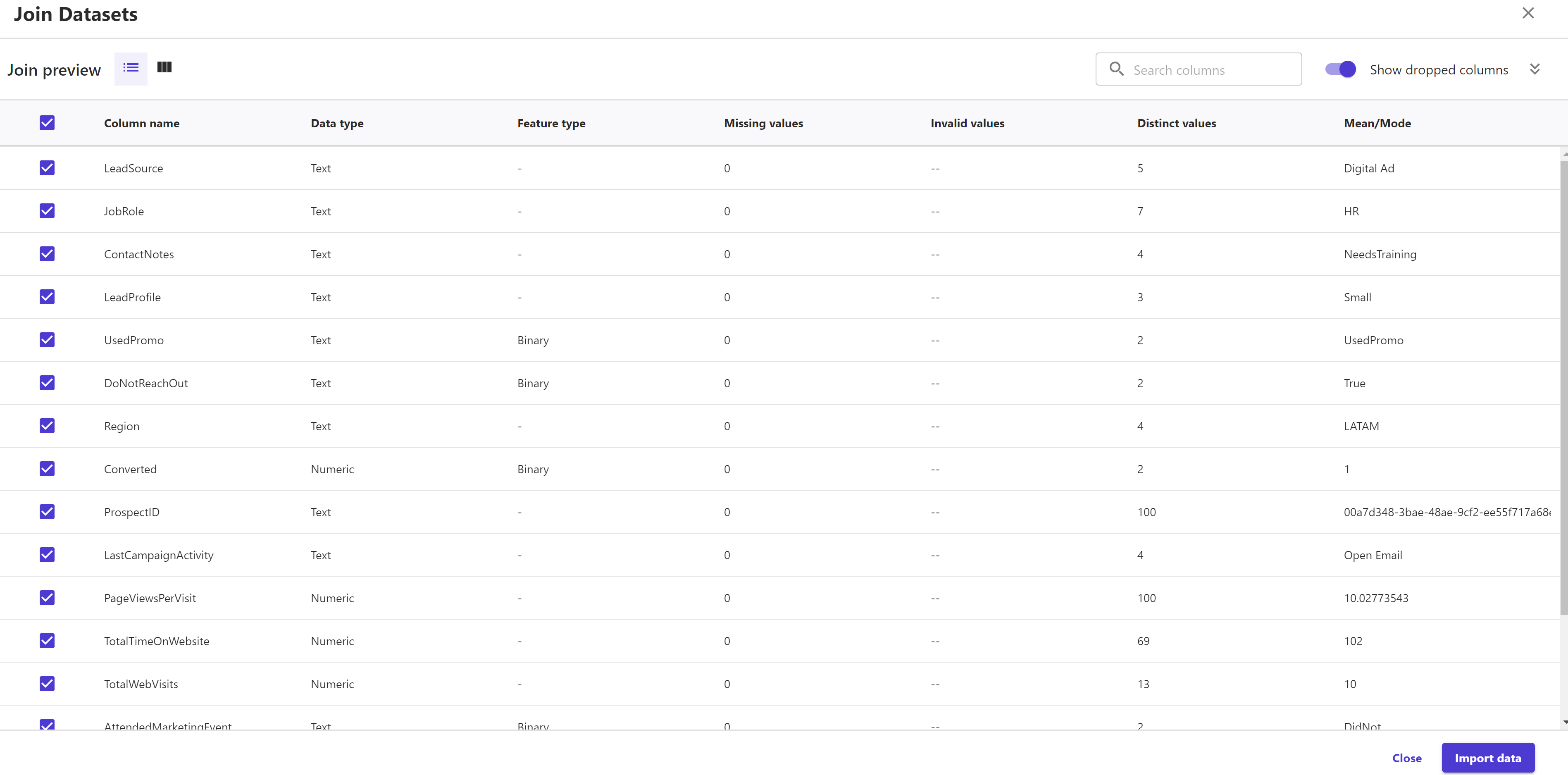
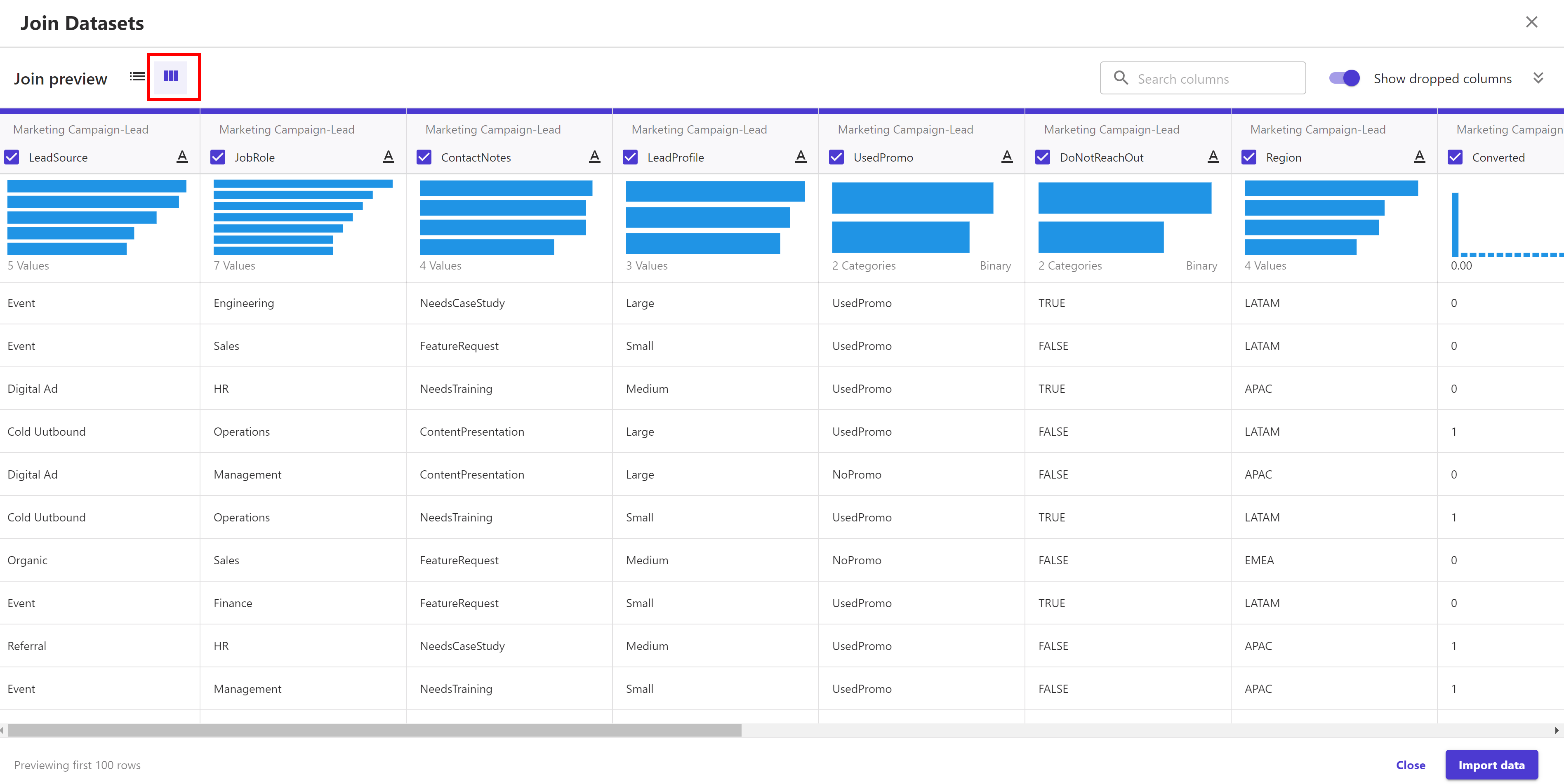
Before importing the data, we can preview the joined dataset in case we want as shown below where it shows statistical data in numerical and graphical forms; for each column in the new dataset. Click on the double arrows to expand the join preview section:
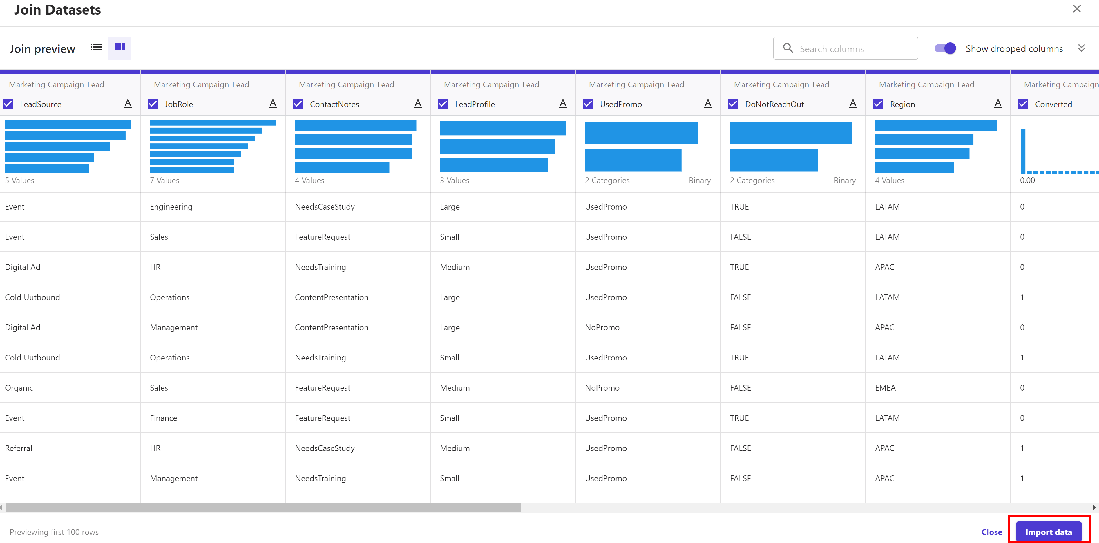
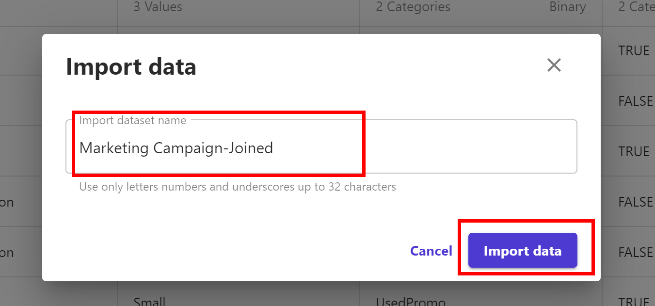
Click on Import data button and provide import dataset name, for example, Marketing Campaign-Joined, and the click Import data again.
Once finished, we can see the new dataset in the Datasets page.
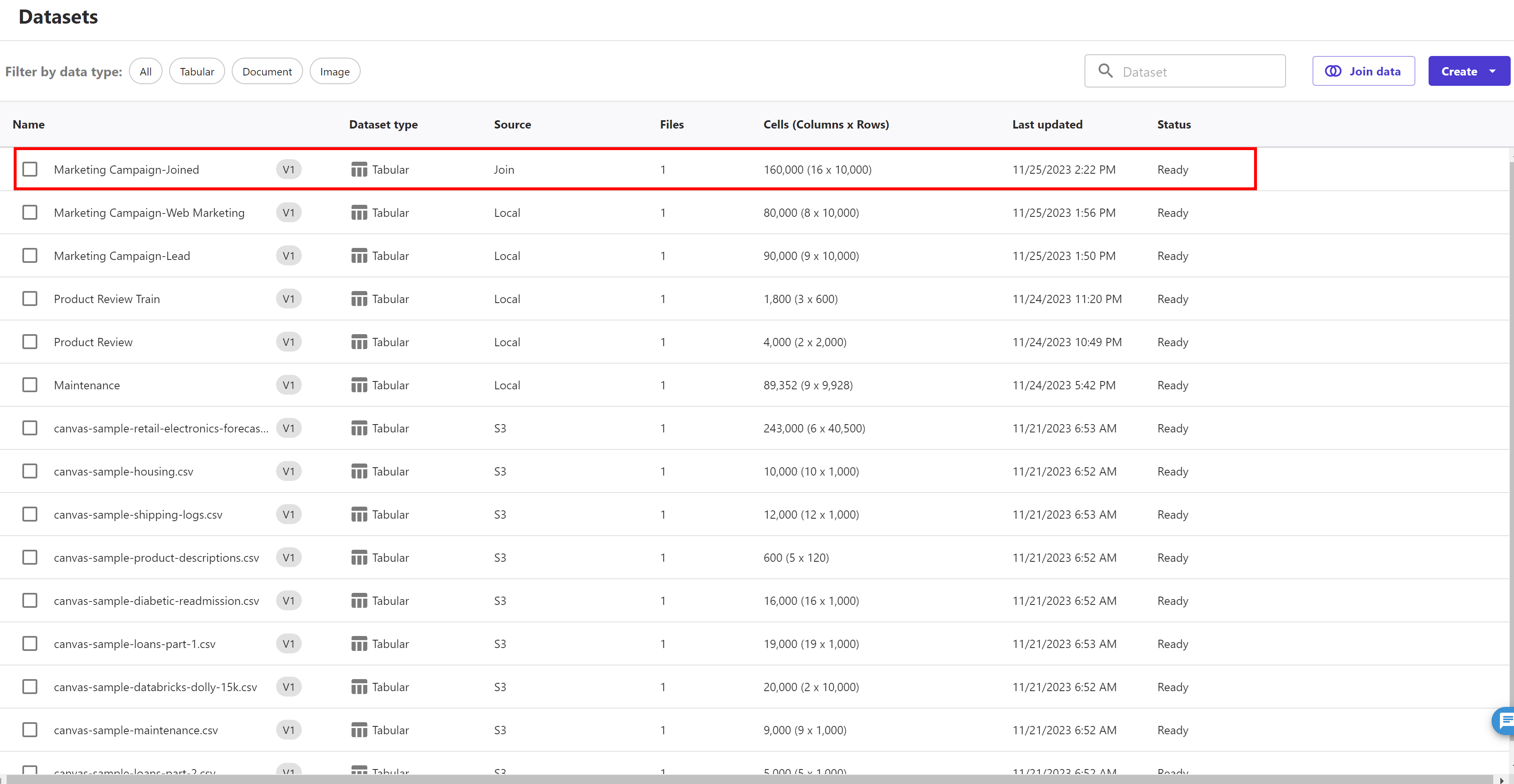
We can use this new dataset to train our model.
Now, let's start building our model.
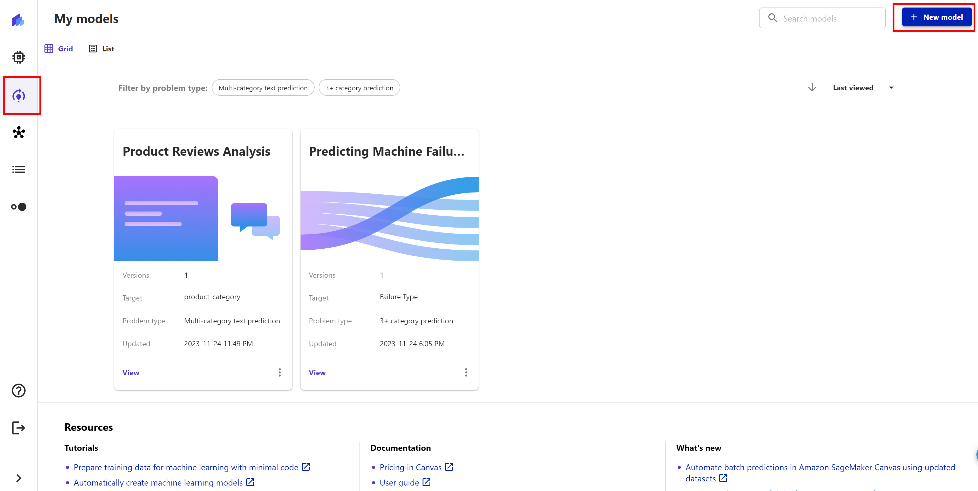
In the left panel, click My models icon, and the click + New model.
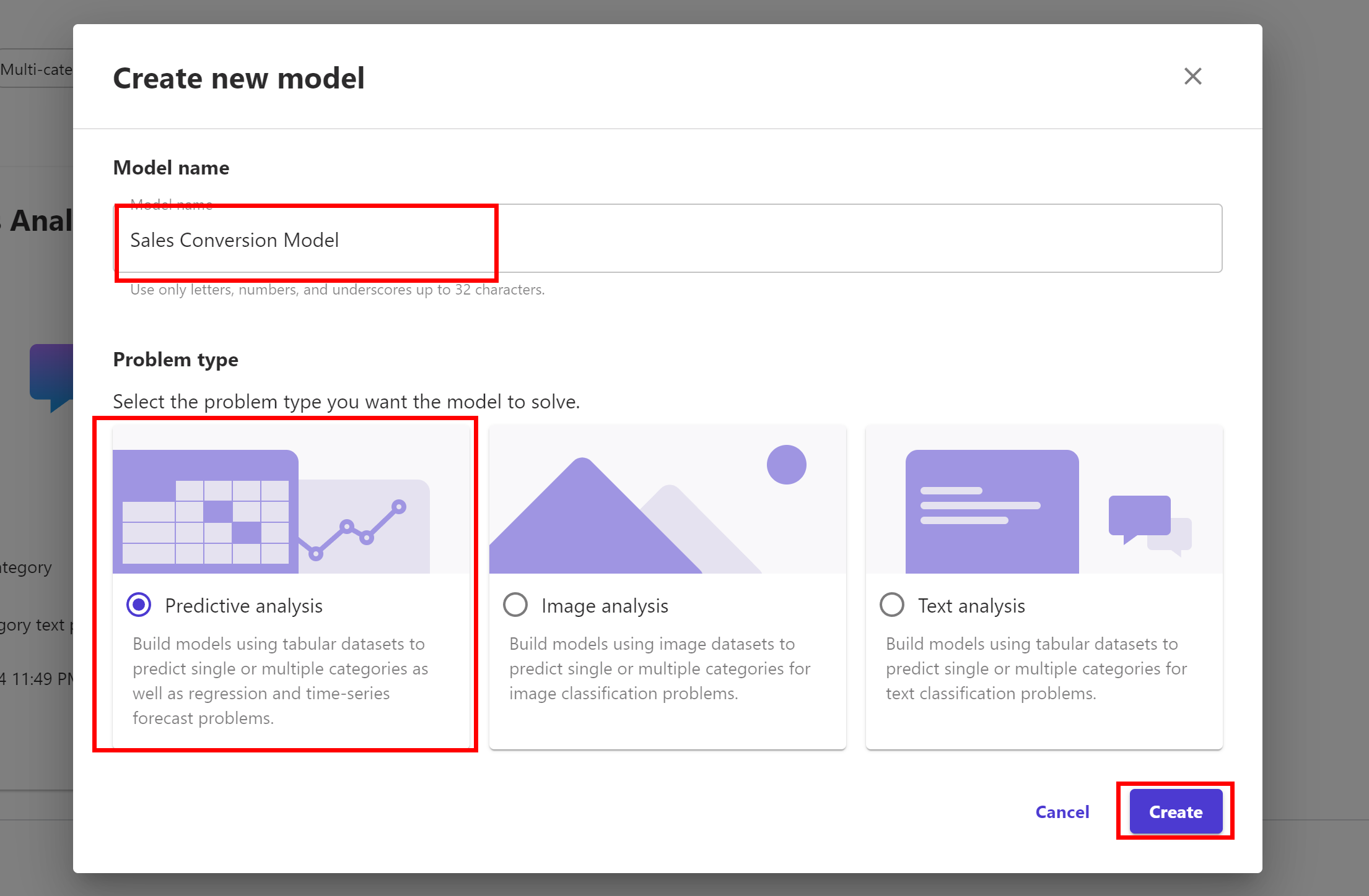
Give our model a name, for example, Sales Conversion Model. For the model type, we choose, Predictive analysis. Then click Create.
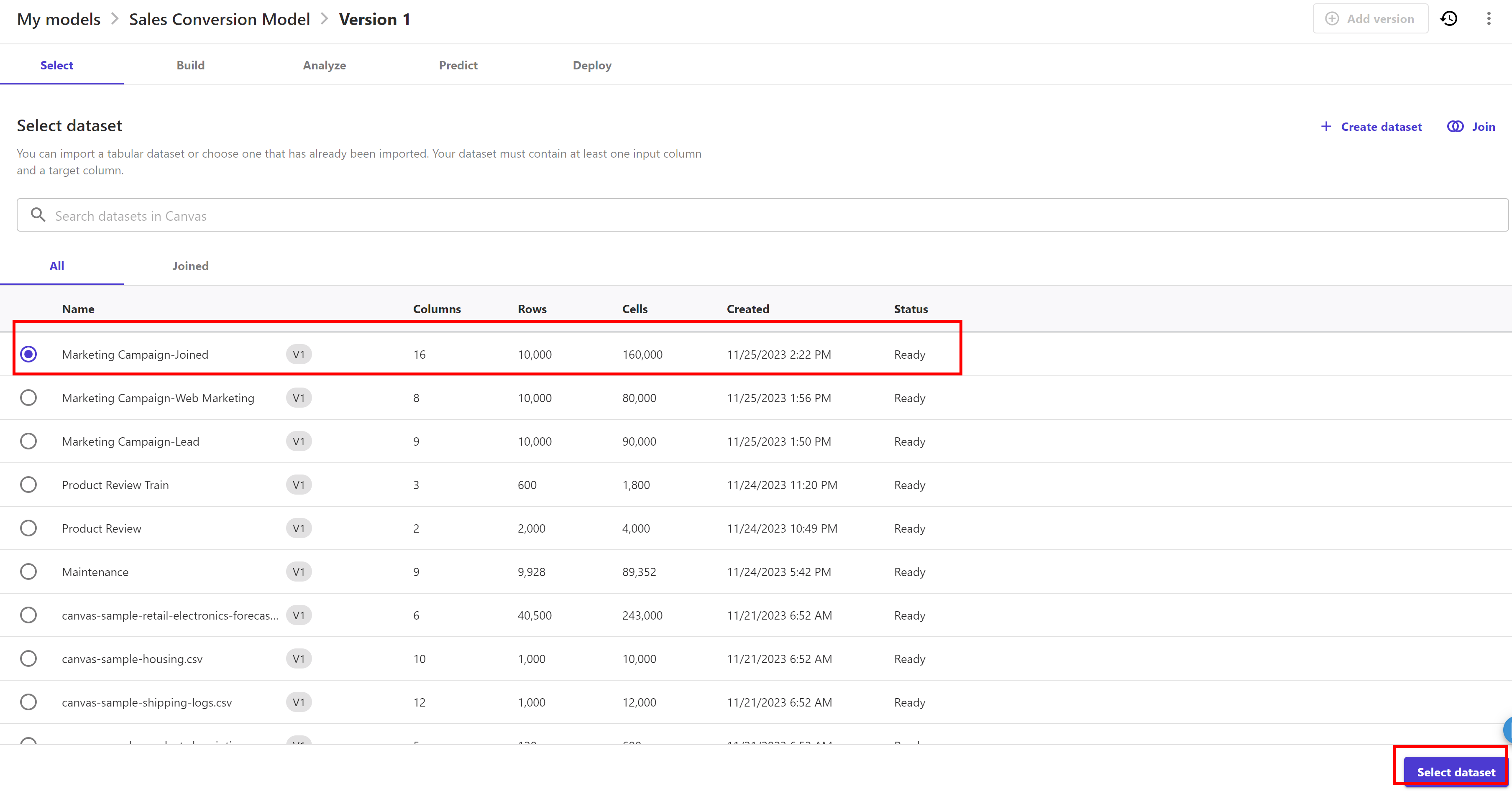
Then select the Marketing Campaign-Joined dataset we just created and click Select dataset
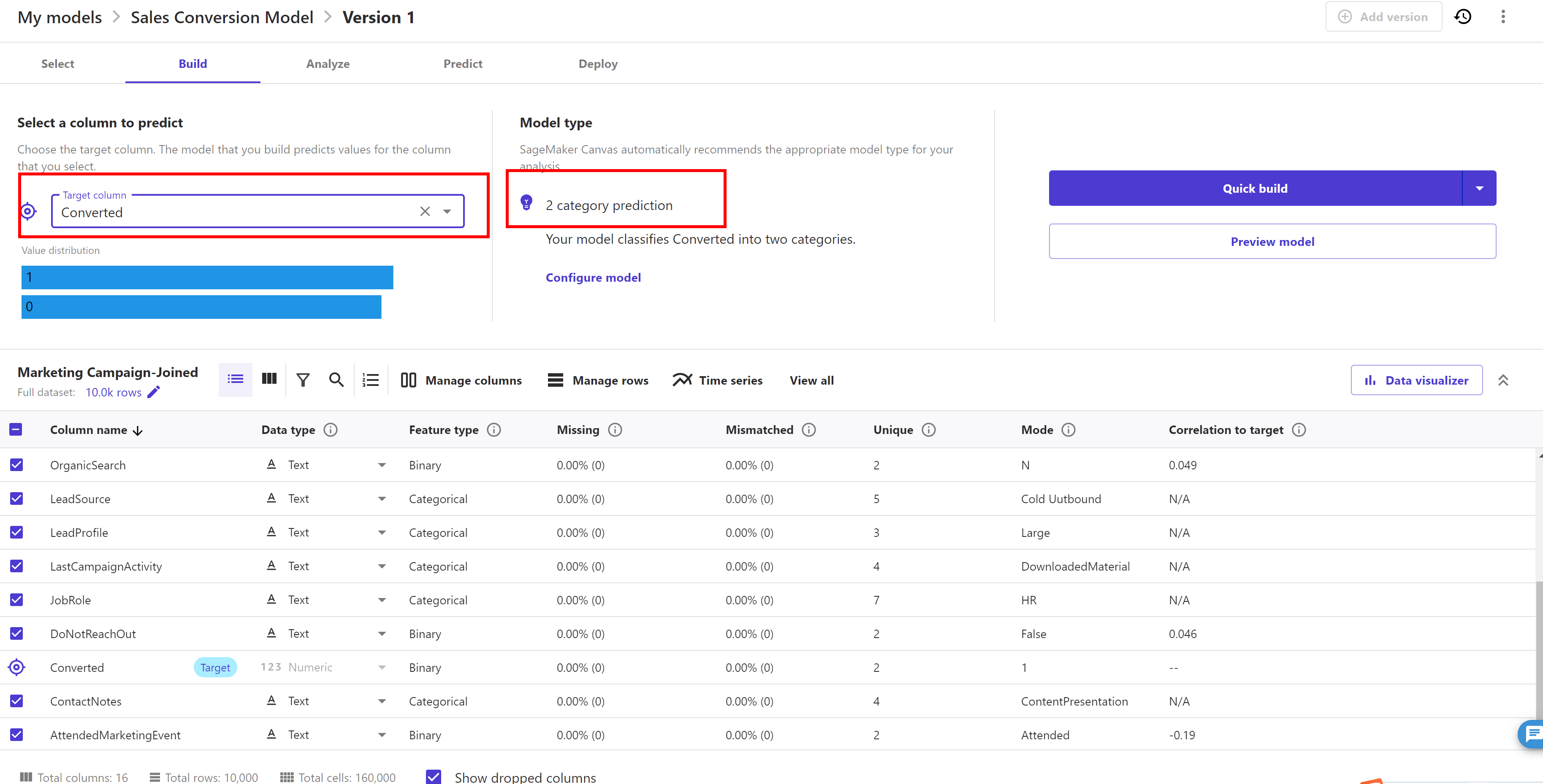
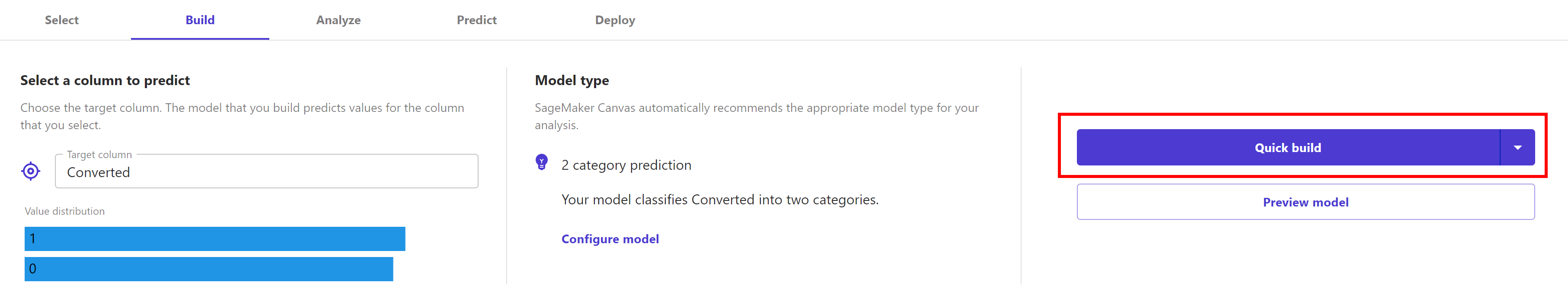
Select the Target column as "Converted". SageMaker Canvas automatically detects that this is a 2 Category problem.
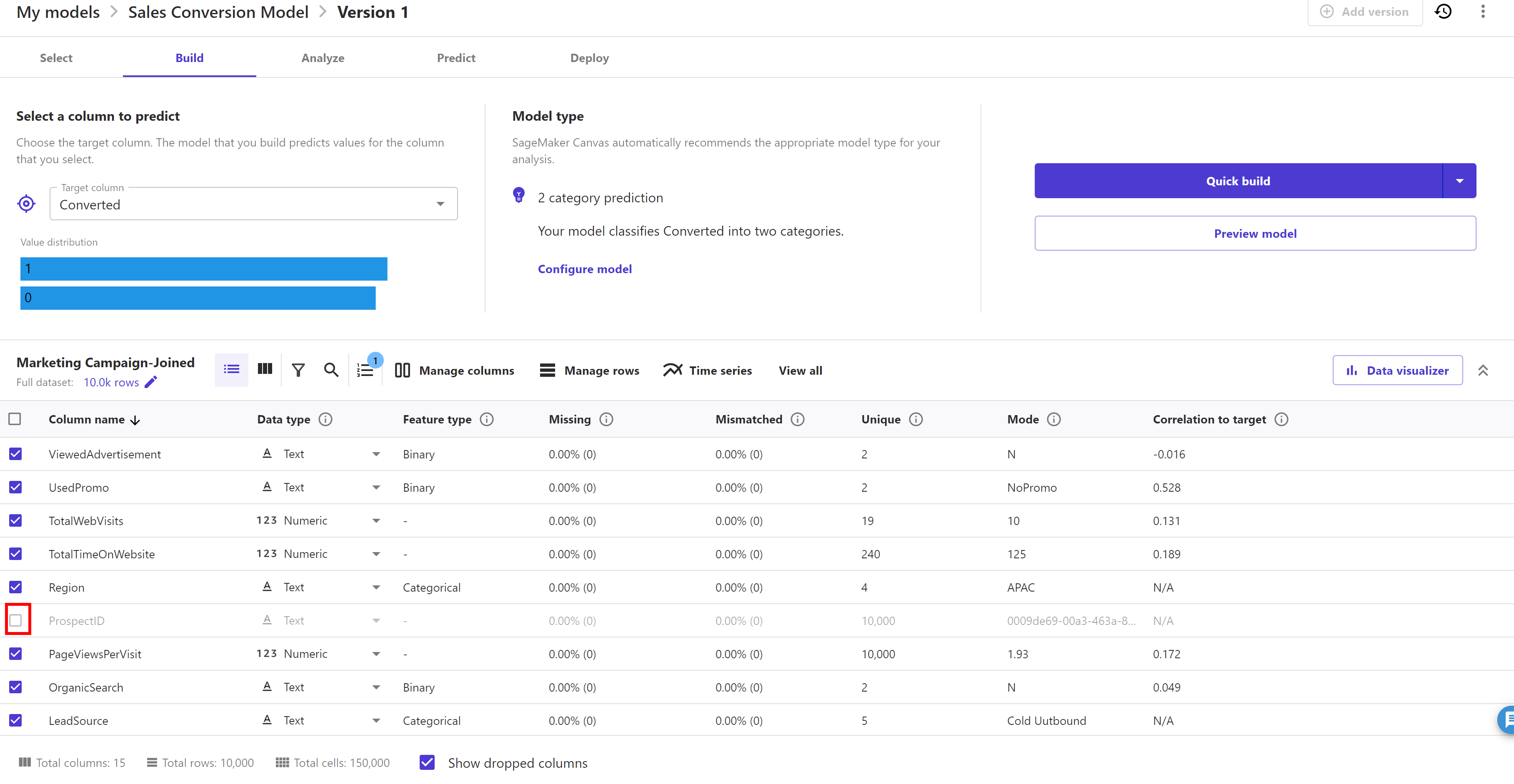
Remove the select mark against the 'ProspectID' field as it doesn't have any impact on 'converted' target feature and hence not required to train the model.
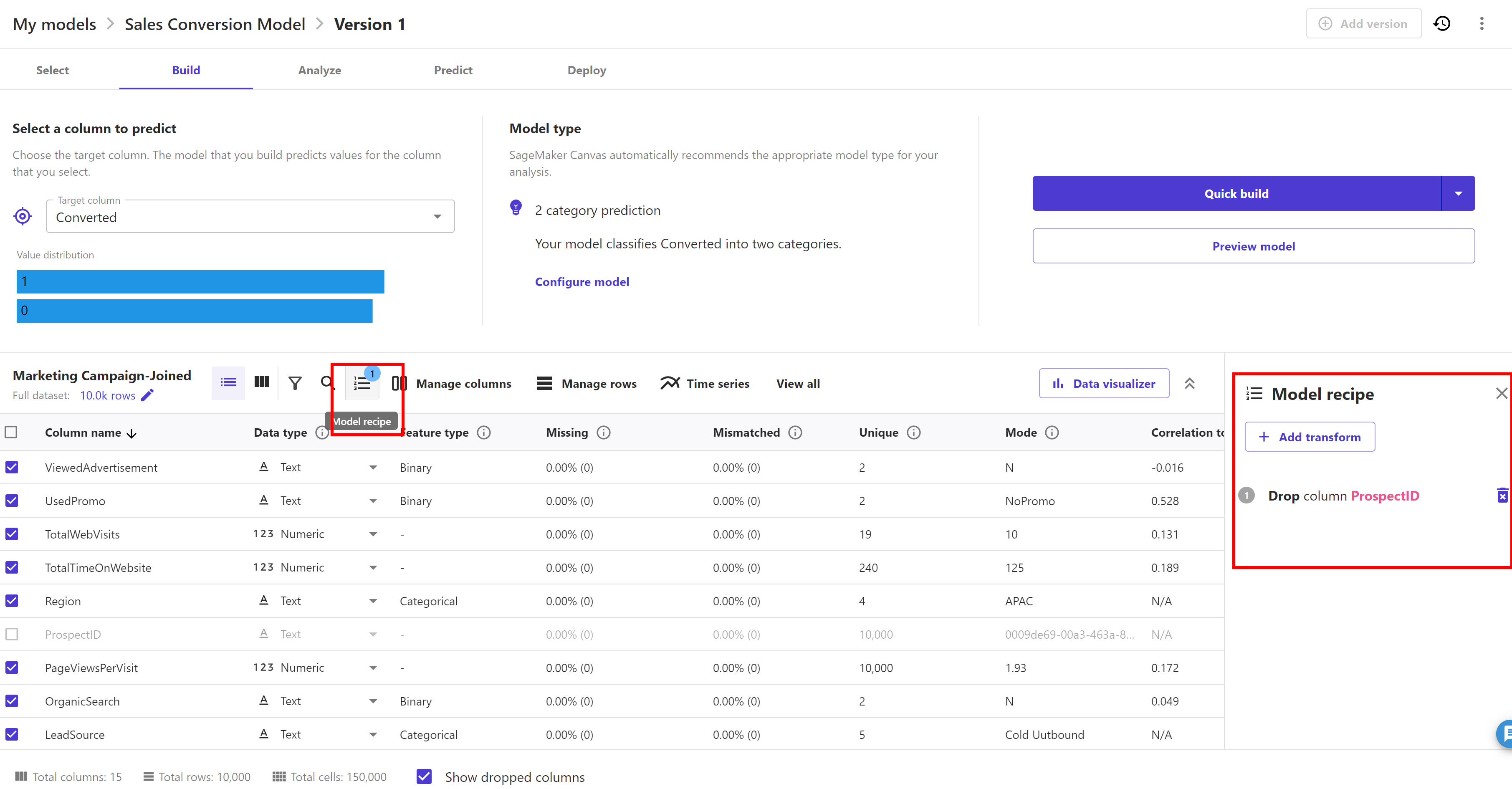
Click on "model recipe" button which demonstrates that ProspectID feature is dropped now.
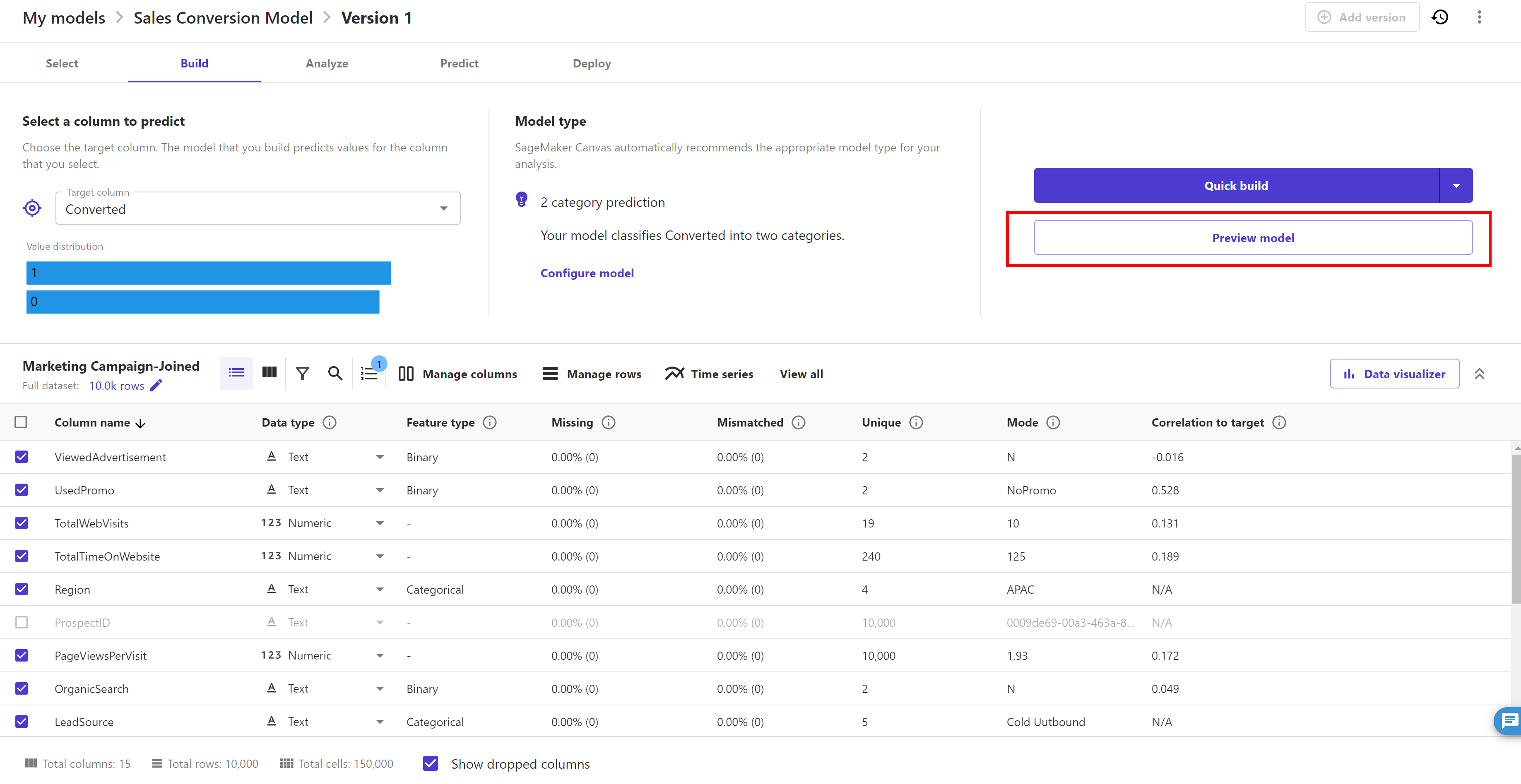
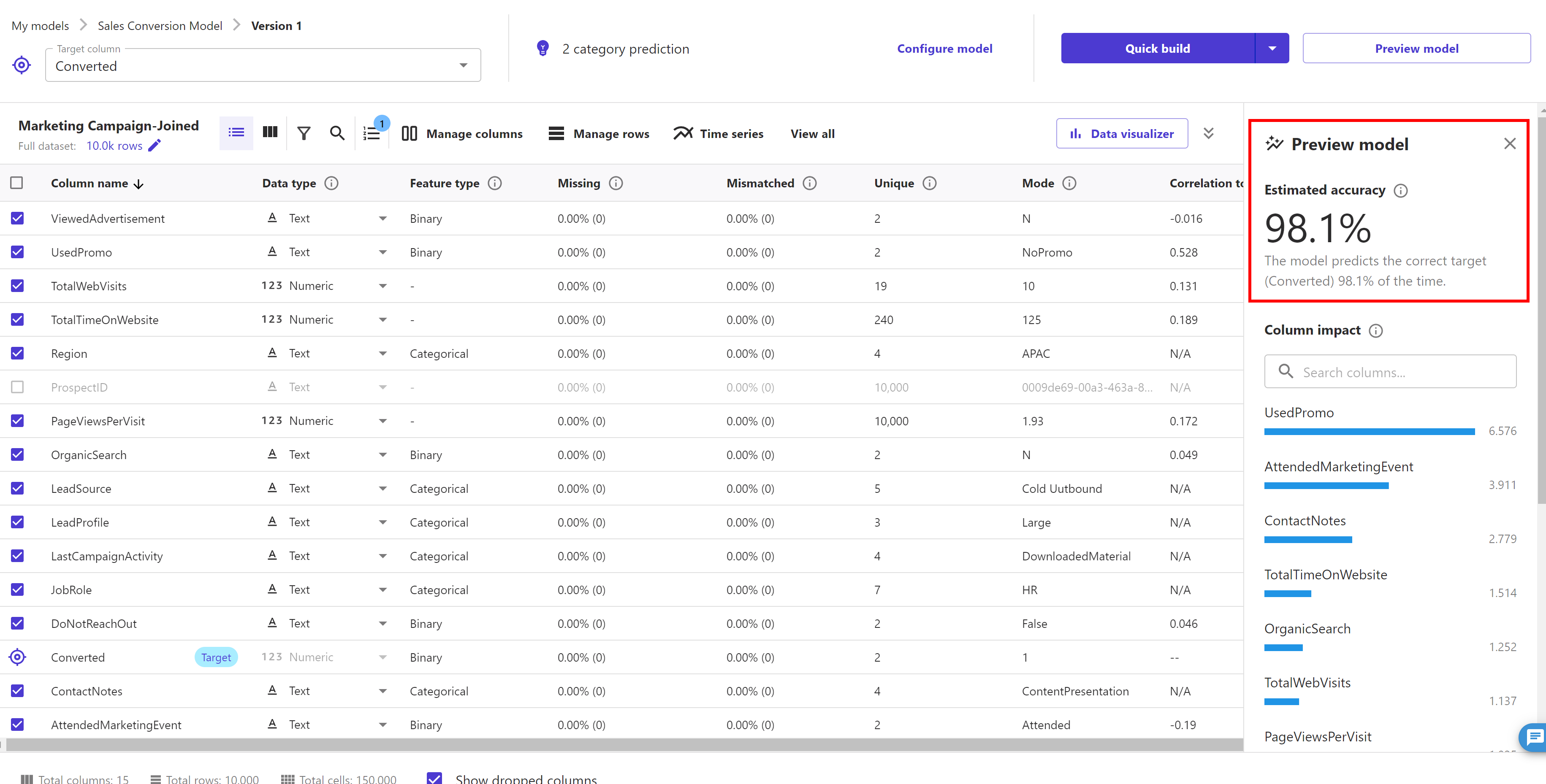
Before going ahead to build a model, SageMaker Canvas provides us functionality of previewing our model before building it. SageMaker Canvas gives us the ability to get insights from our data before we build a model by choosing Preview model. For example, we can see how the data in each column is distributed. For models built using categorical data, we choose Preview model to generate an Estimated accuracy prediction of how well the model can analyze our data. SageMaker Canvas uses a subset of our data to build a model quickly to check if our data is ready to generate an accurate prediction. Using this sample model, we can understand the current model accuracy and the relative impact of each column on predictions.
As we can see here that the accuracy is quite good (your model accuracy and column impact order may differ from here as it depends what sample dataset was picked by preview mode functionality.
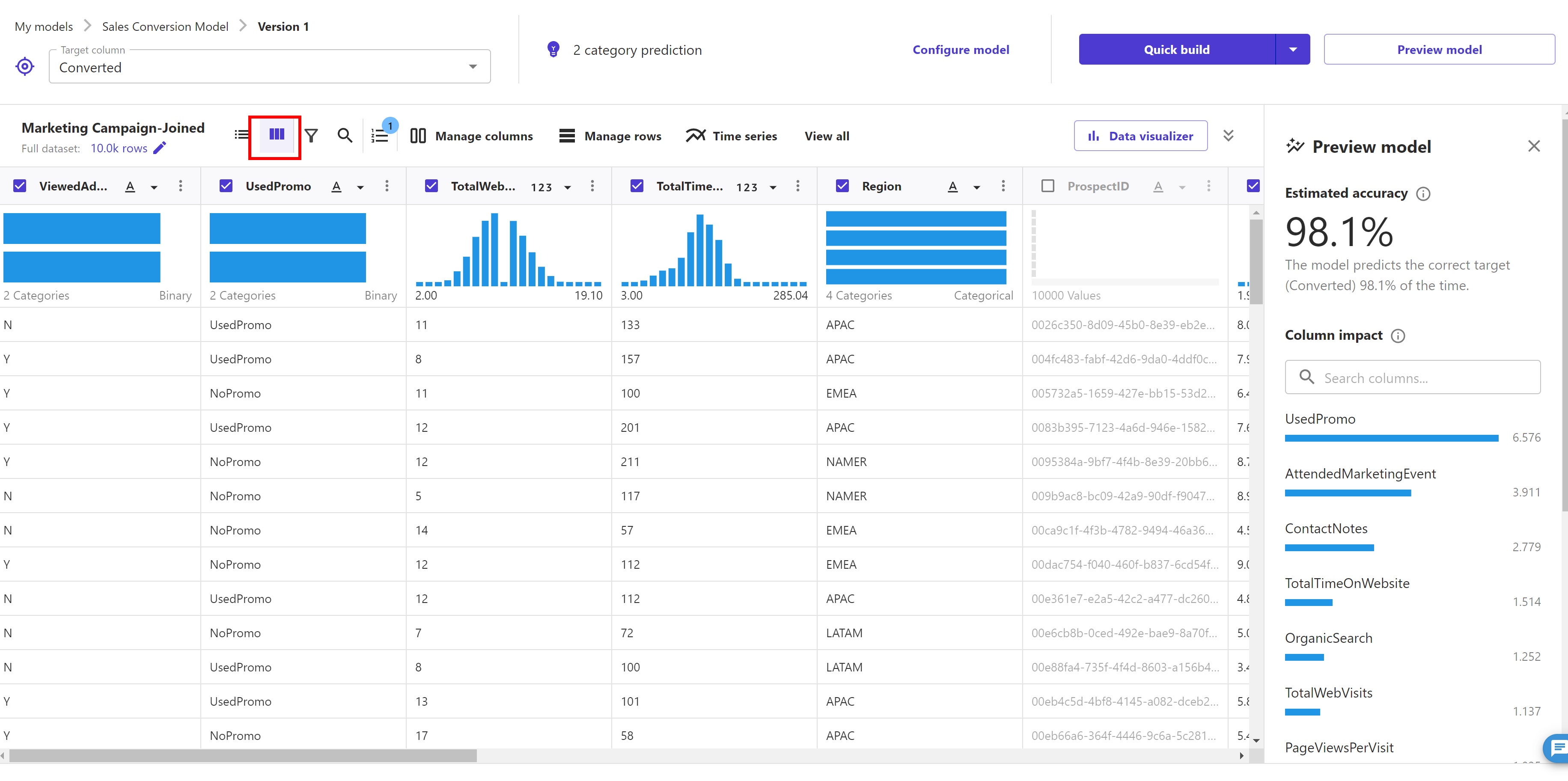
We can also select the "Grid View" to see how the data in each column is distributed.
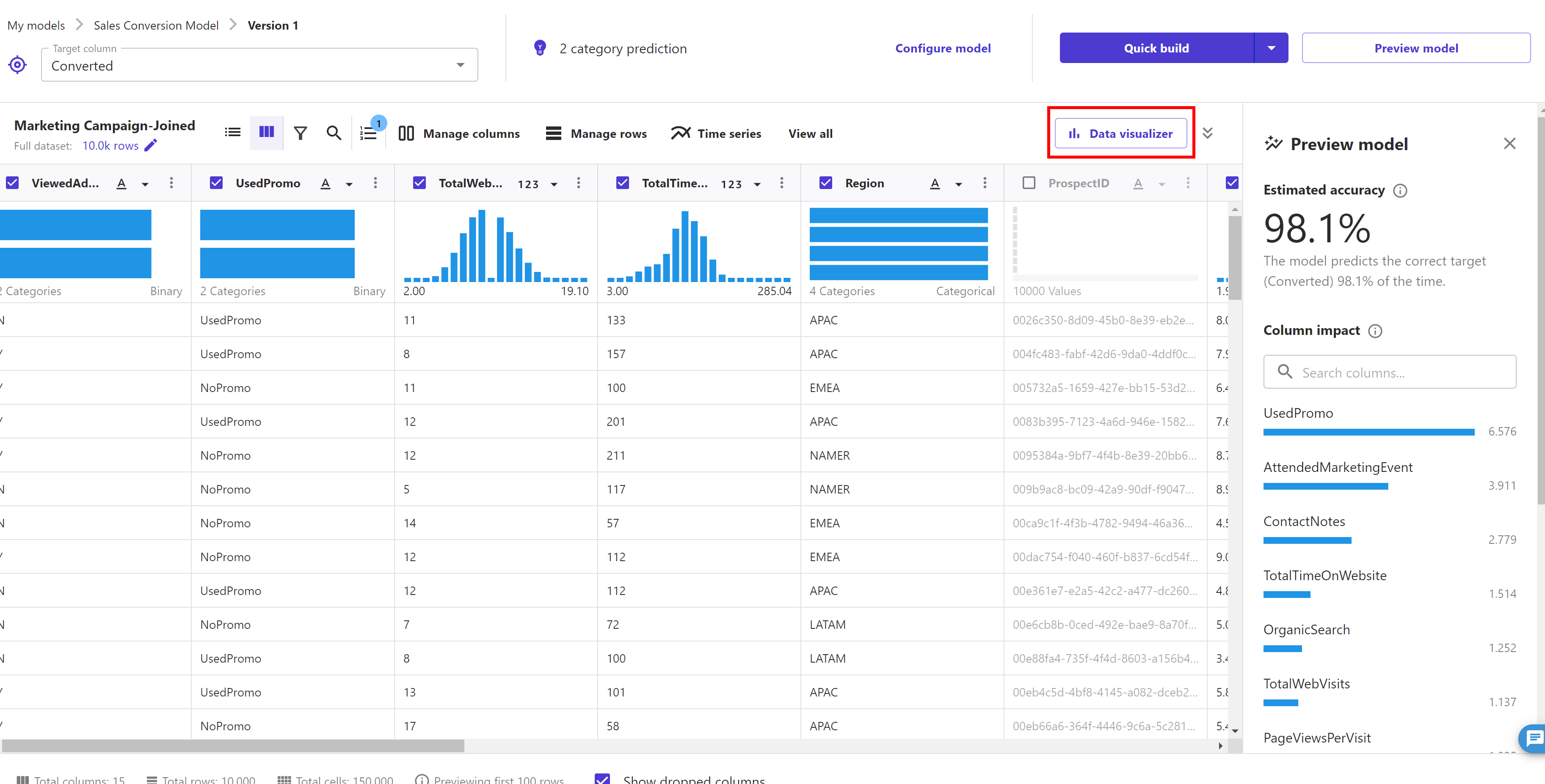
Now click on the "Data visualizer" button. This feature in Canvas allows us to see if there are relationship between elements. We can explore and visualize our data, to help us gain advanced insights into our data before building your ML models. We can visualize using scatter plots, bar charts, and box plots, which can help us understand our data and discover the relationships between features that could affect the model accuracy.
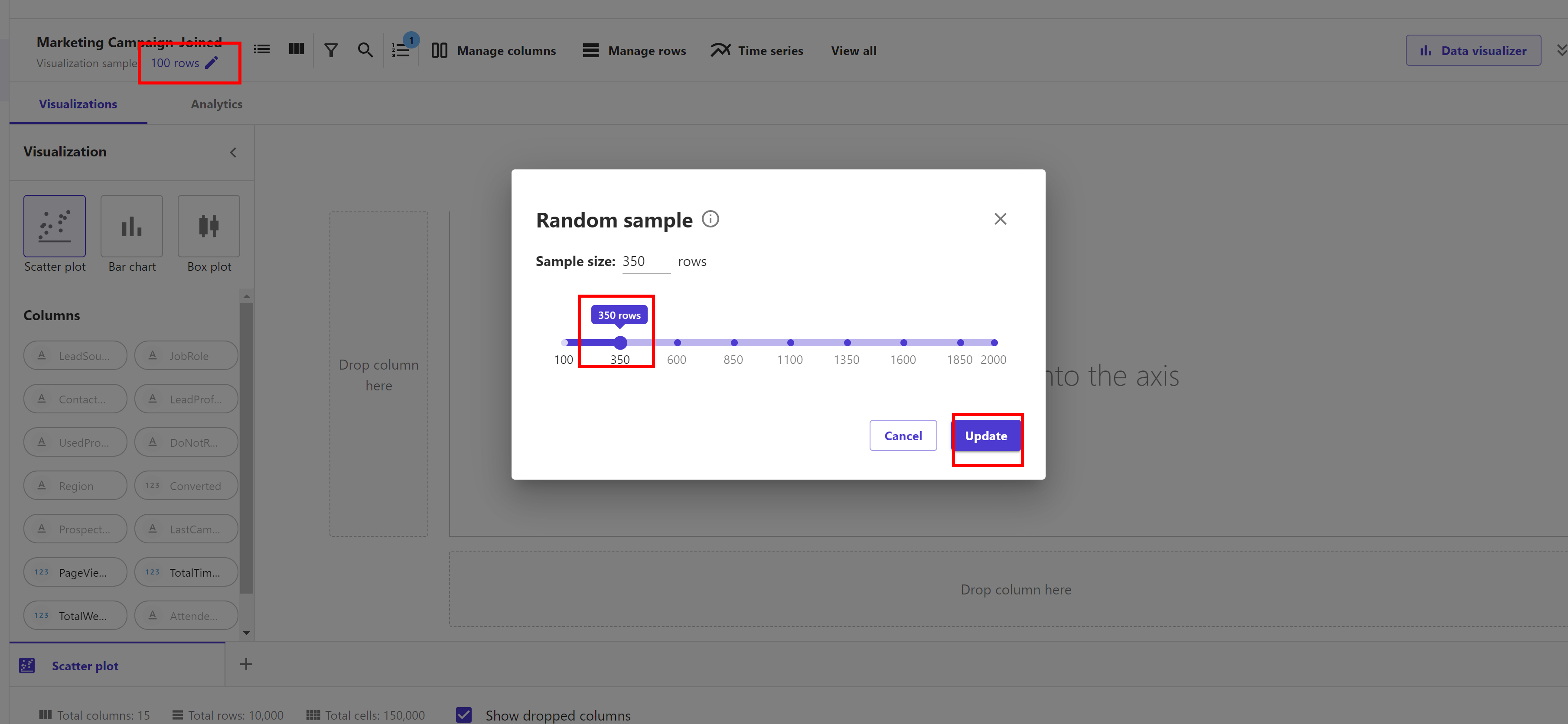
We can change the sample size based on our dataset to get a better perspective. To do this in the Data Visualizer choose number of rows next to Visualization sample and then use the slider to select our desired sample size. For example, we select 350 rows, click "Update".
Under visualization we can see "Scatter plot" is selected by default. A scatter plot shows the relationship between two quantitative variables measured for the same individuals. In our case, it’s important to understand the relationship between values to check for any correlation. For this we are going to select the column "PageViewsPerVisit" and drag it to the Y axis, and select the column "TotalTimeOnWebsite" and drag it to the X axis.
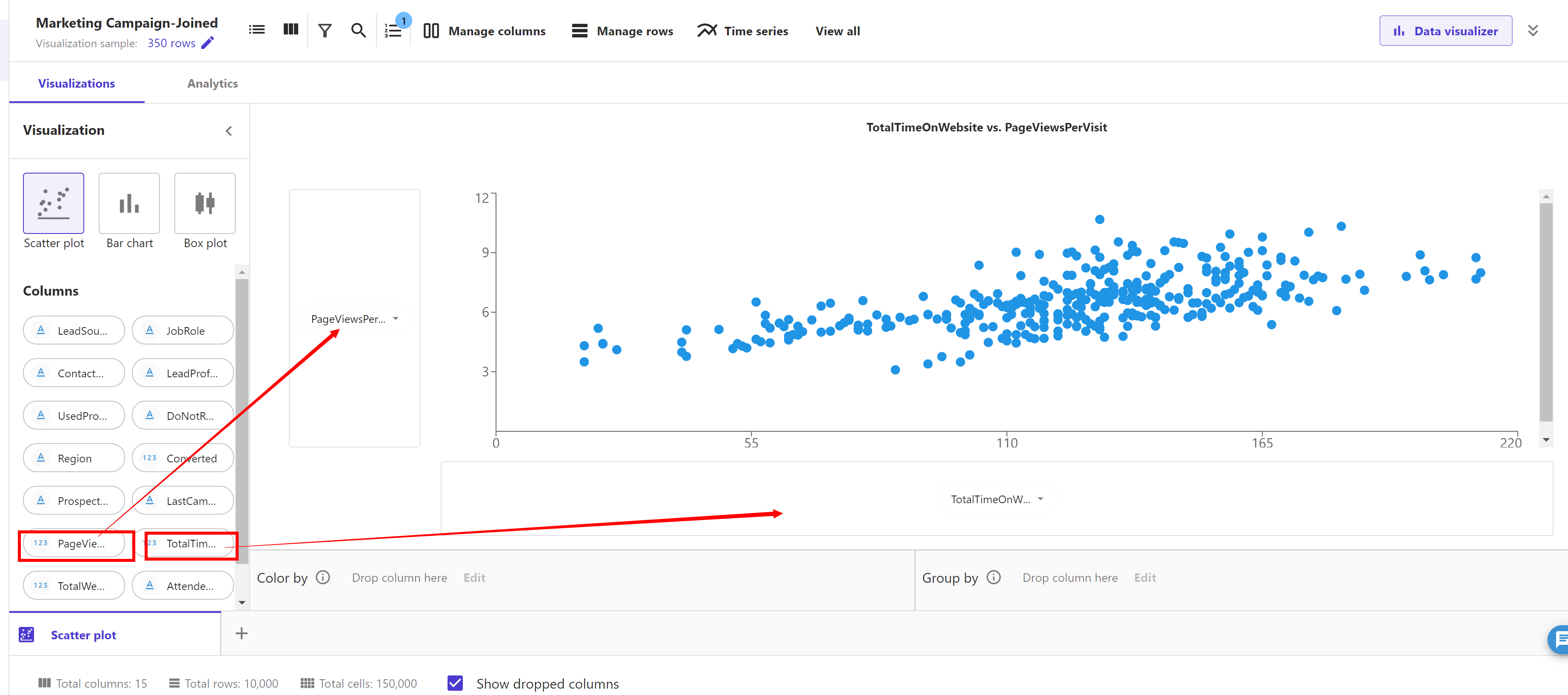
Including feature pairs with high correlation, in some ML algorithms, can take additional storage and reduce the speed of training, and having similar information in more than one column might lead to the model overemphasizing the impacts and lead to undesired bias in the model. For this case we won’t be removing any feature.
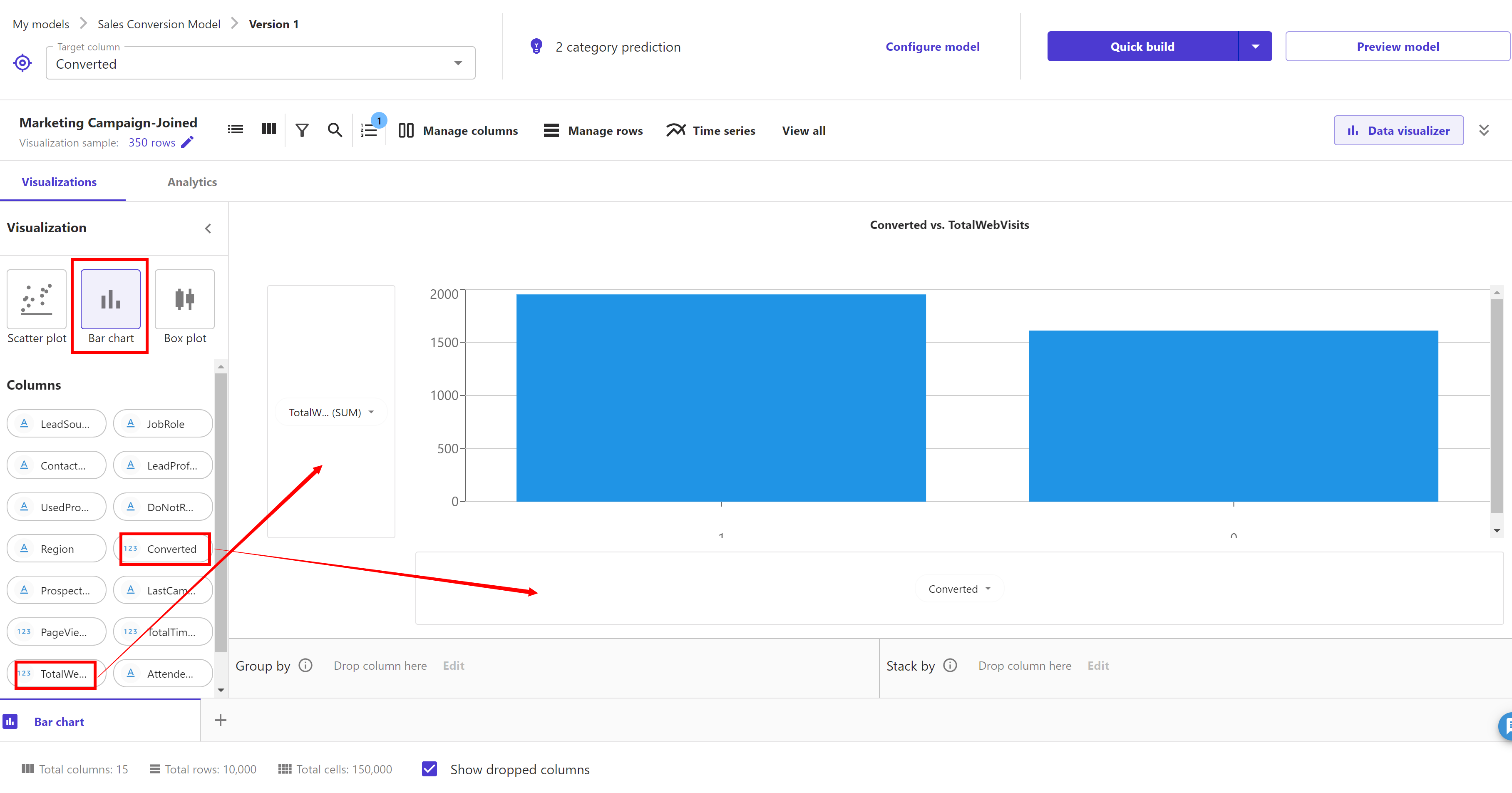
Now let’s look at data balance and variation. We will create a bar chart to see the how the number of web visits are distributed across our target column Converted or not. Under visualization select "Bar chart". Select column "TotalWebVisits" and drag it to the Y axis, and select column "Converted" and drag it to the X axis.
Now, let’s look at Box plots. Select "Box Plots" and drag and drop "TotalTimeOnWebsite" and "Converted" to the y-axis and x-axis, respectively.
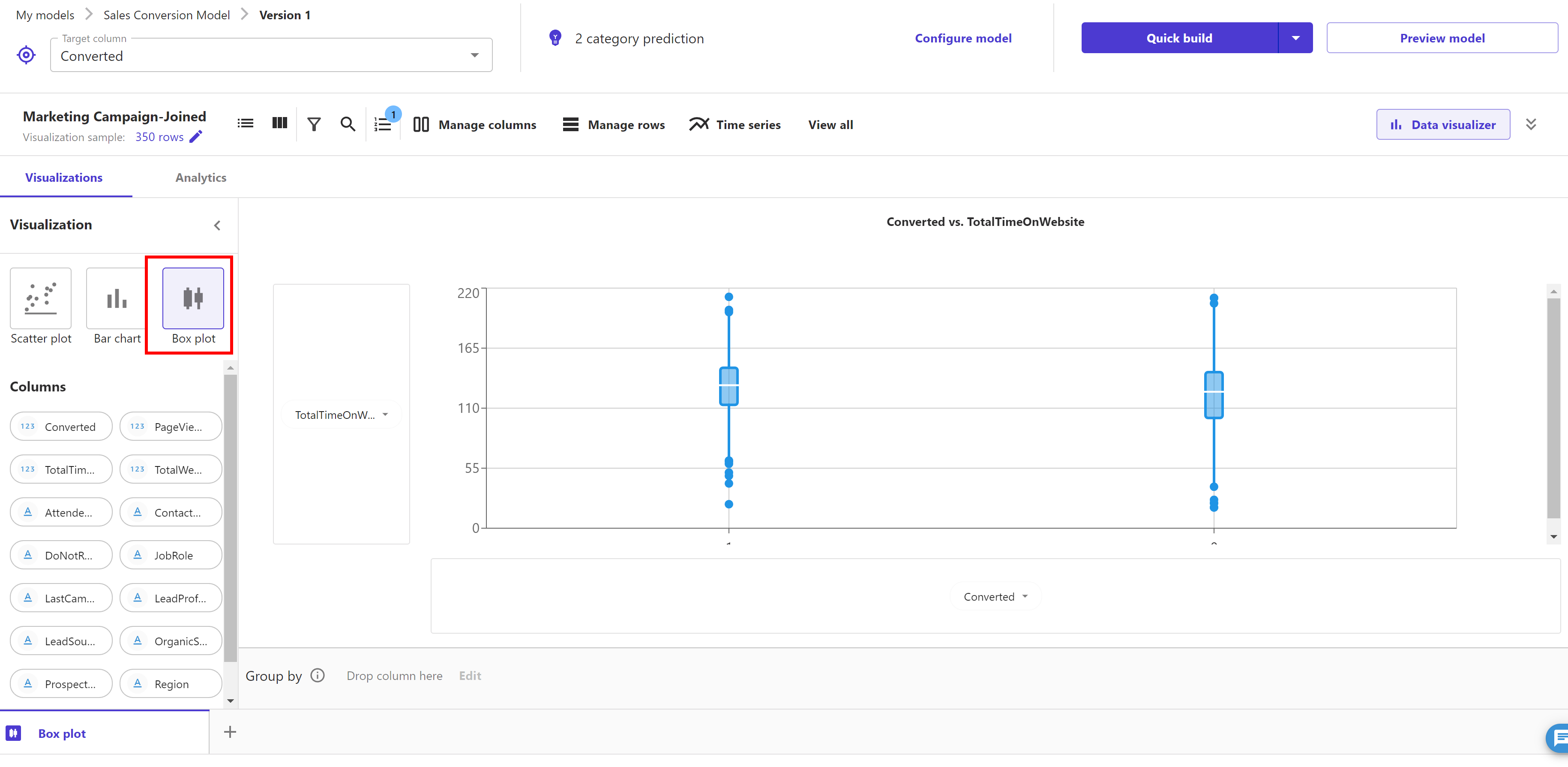
Box plots are useful because they show differences in the behaviour of data by class (churn or not). Because we’re going to predict churn (target column), let’s create a box plot of some features against our target column to infer descriptive statistics on the dataset, such as mean, max, min, median, and outliers.
From our observations, we can determine that the dataset is fairly balanced. We want the data to be evenly distributed across true and false values so that the model isn’t biased towards one value. Now we are ready to build the model.
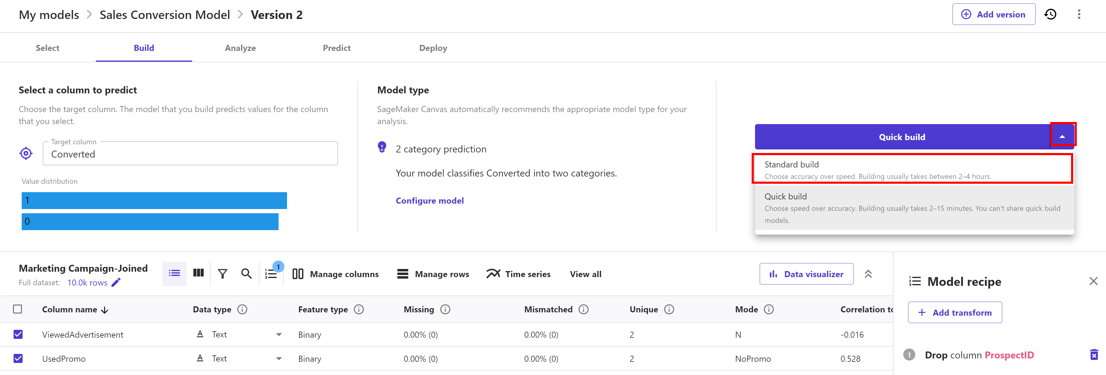
Click on the arrow of "Quick build" button and we will see 2 options to build the model. First one is the Standard build and second one is Quick build.
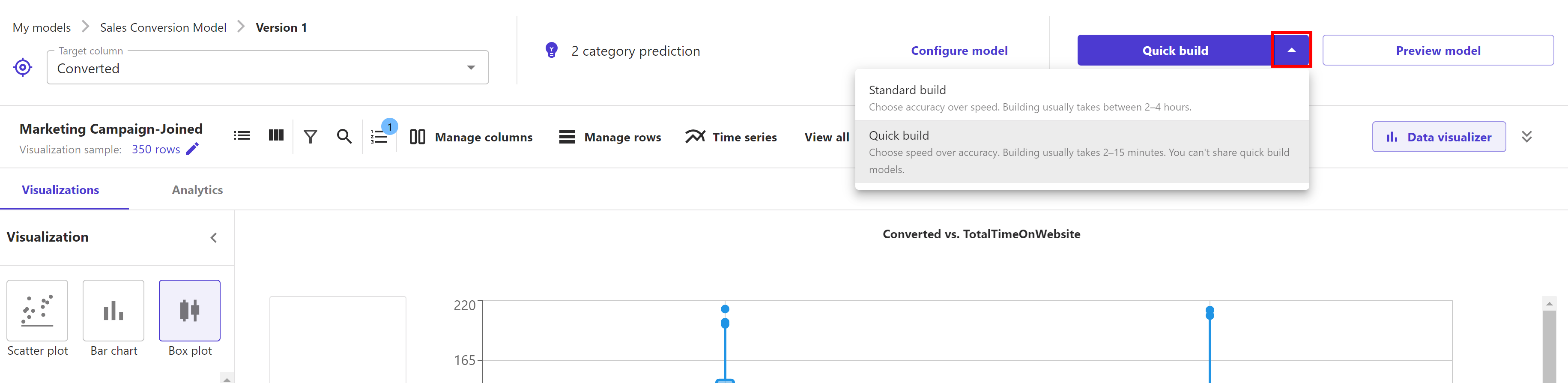
For now, we will use the "Quick build". Click on the "Quick build" button and it starts building the model. It takes around 5-10 minutes to complete.
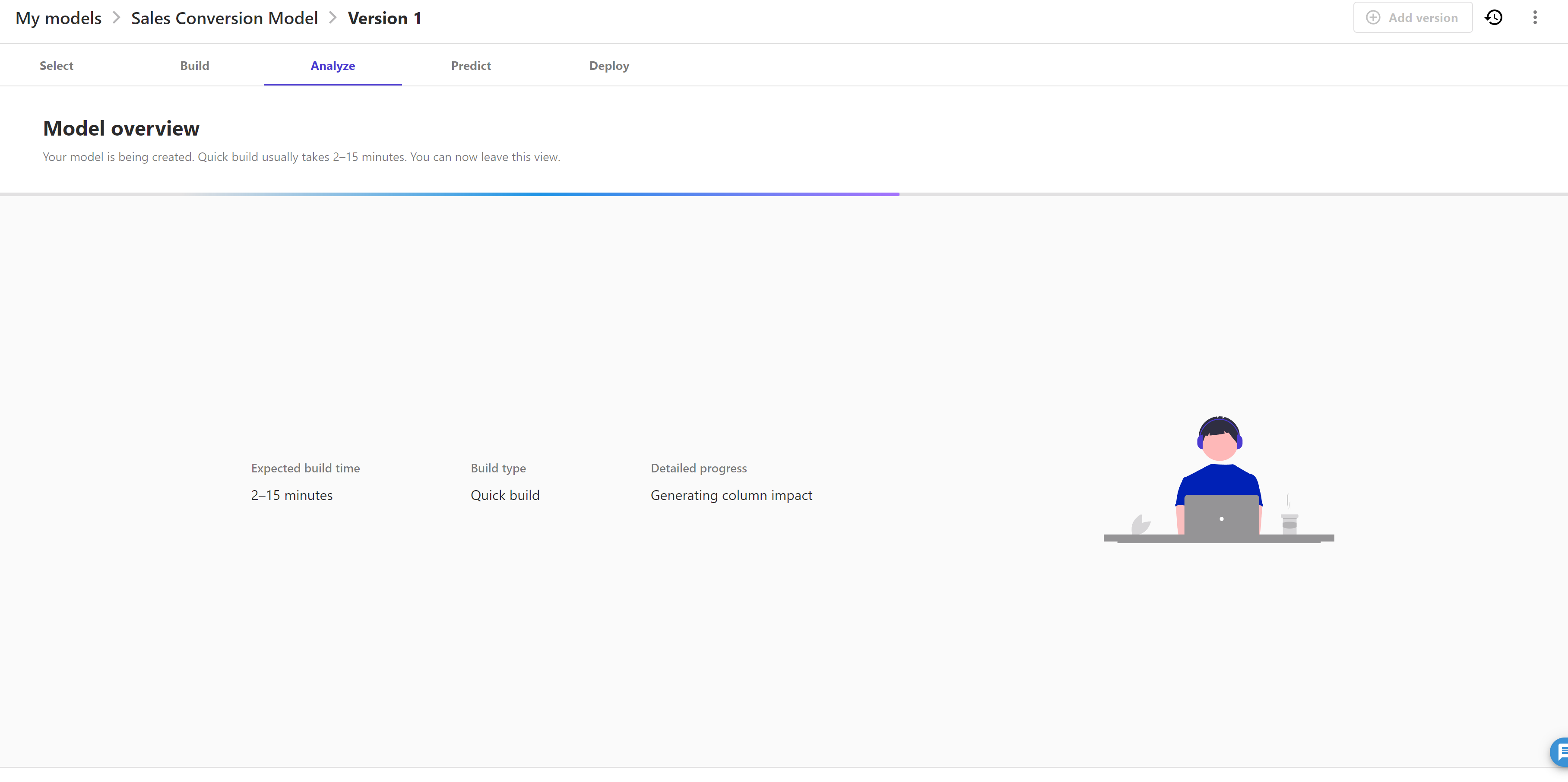
Once model build is complete we can see estimated accuracy and column impact list as below.
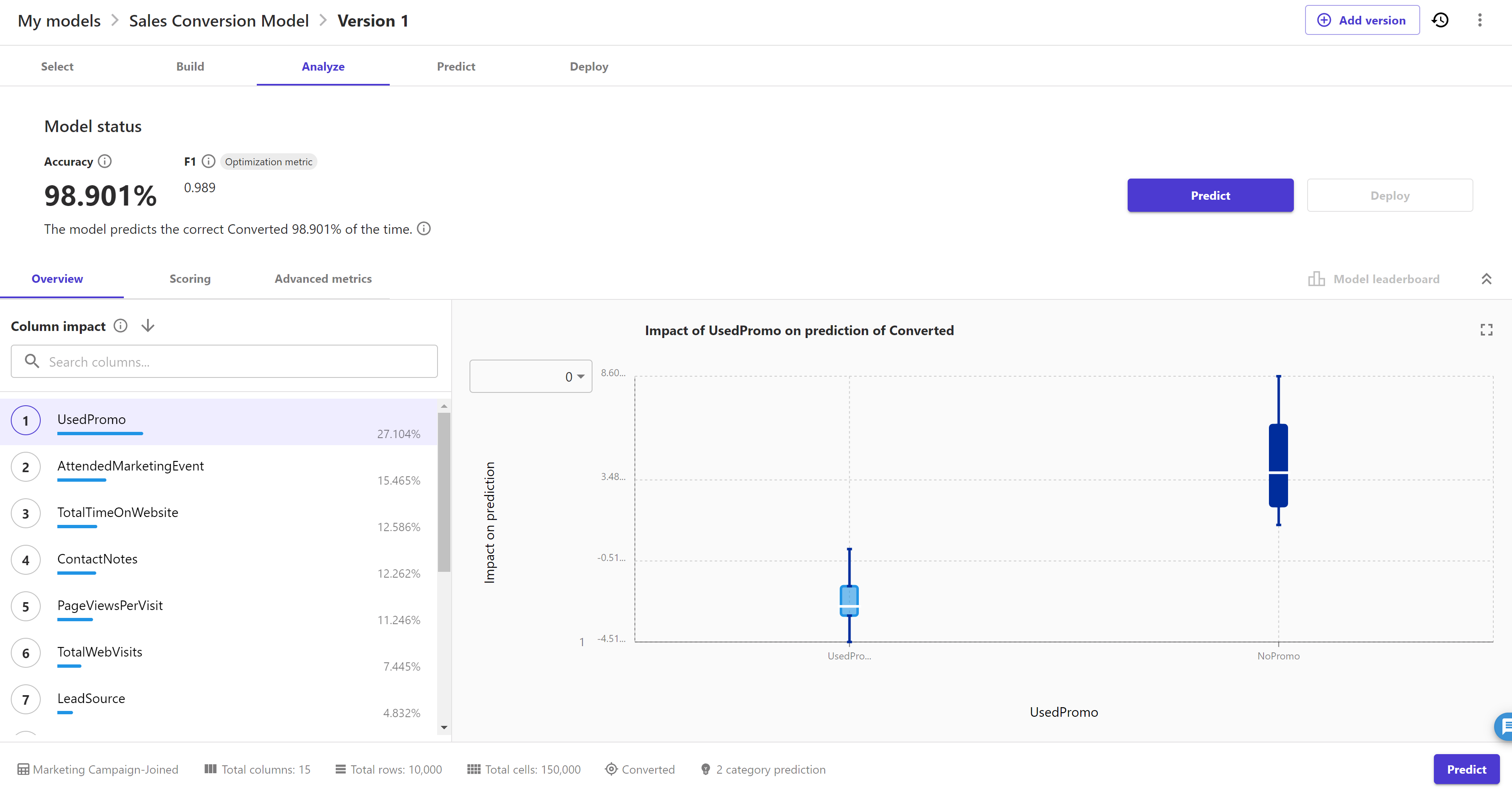
We evaluate how well our model performed on our data before we start using it to make predictions by using the following:
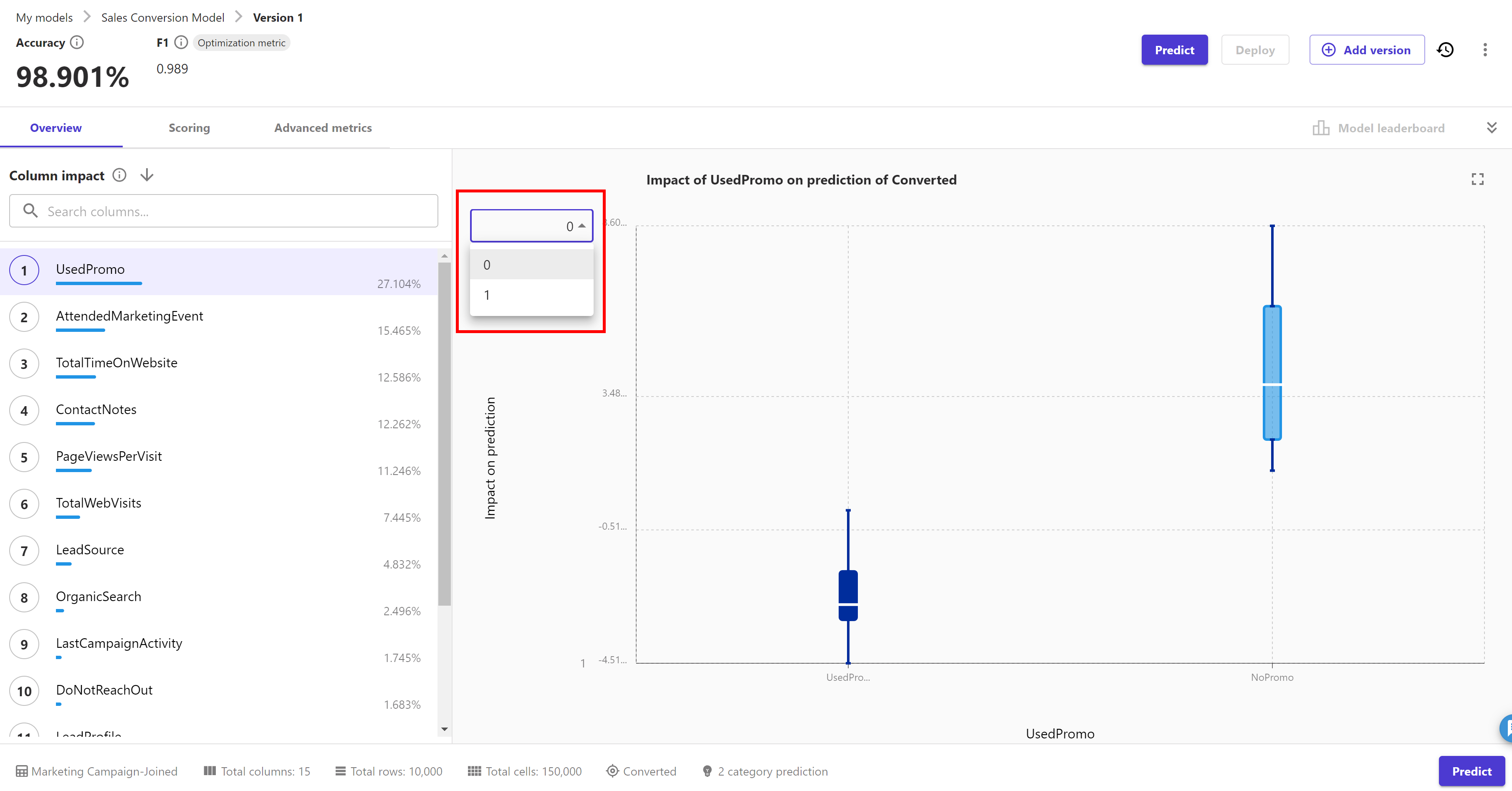
Scroll down through the "Column impact" order list that depicts which feature has high impact on the inference of target feature using this model. We can click on any column and change the target value ( 0 or 1 ) to see the column impact:
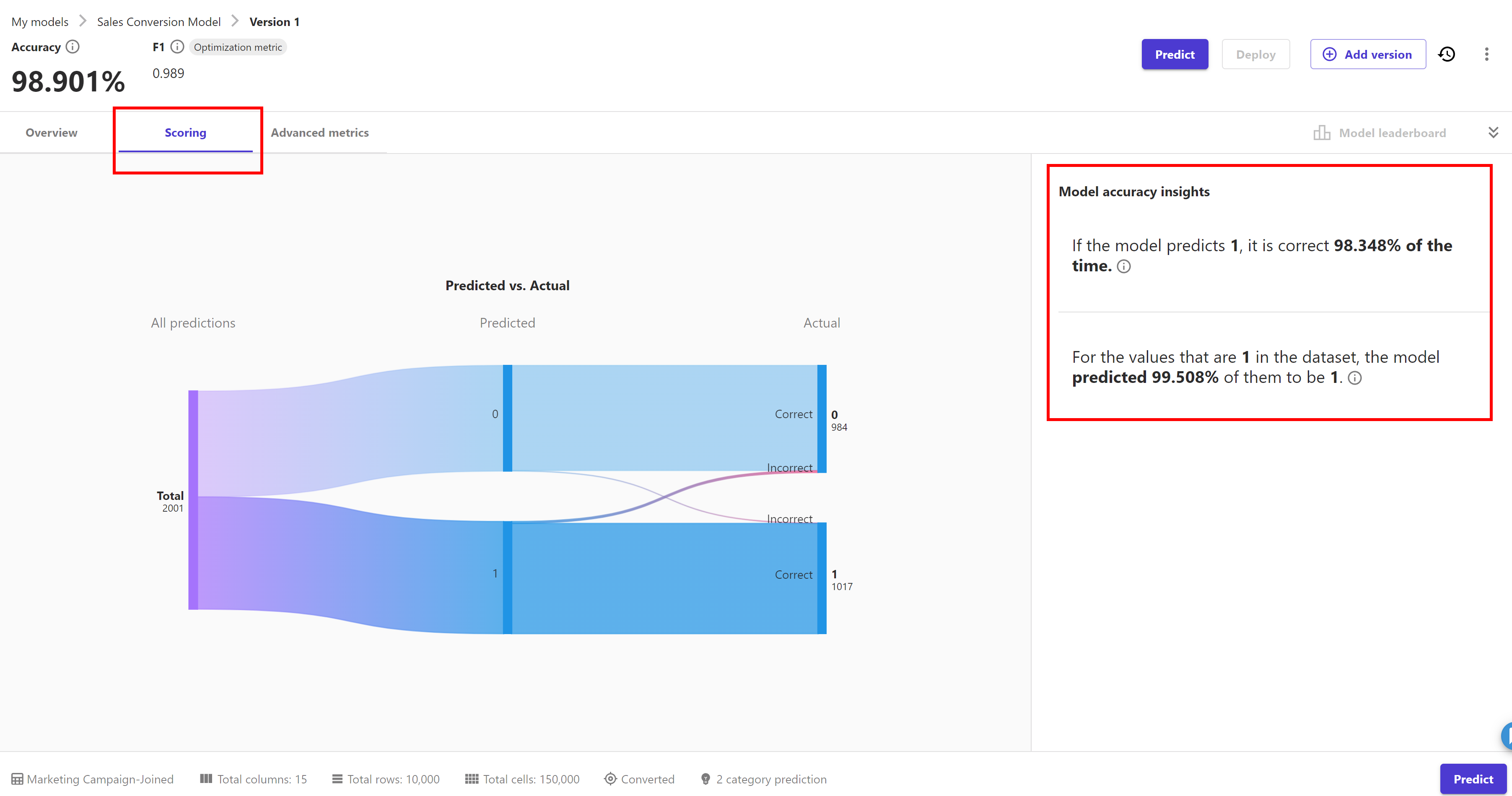
Click on the "Scoring" tab. Here we can see on the right hand side, model accuracy insights are provided to gain more insights of the model.
Now click on the "Advanced metrics" tab. It gives us the information like below:
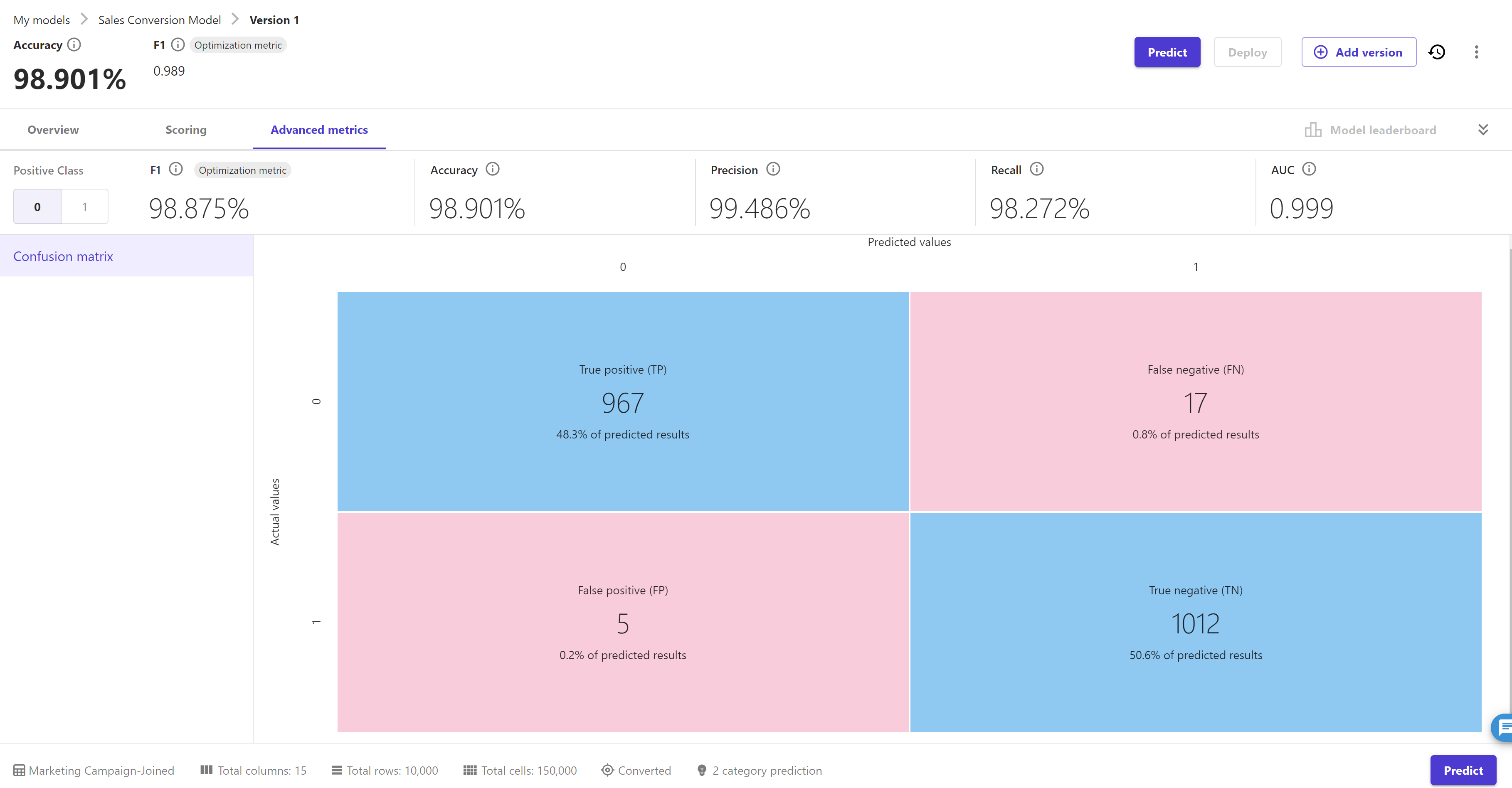
SageMaker Canvas uses confusion matrices to help you visualise when a model makes predictions correctly. As this is a binary classification problem hence advance metrics like F1 score, Accuracy, Precision, recall and AUC are shown above. We can switch the "Positive Class"
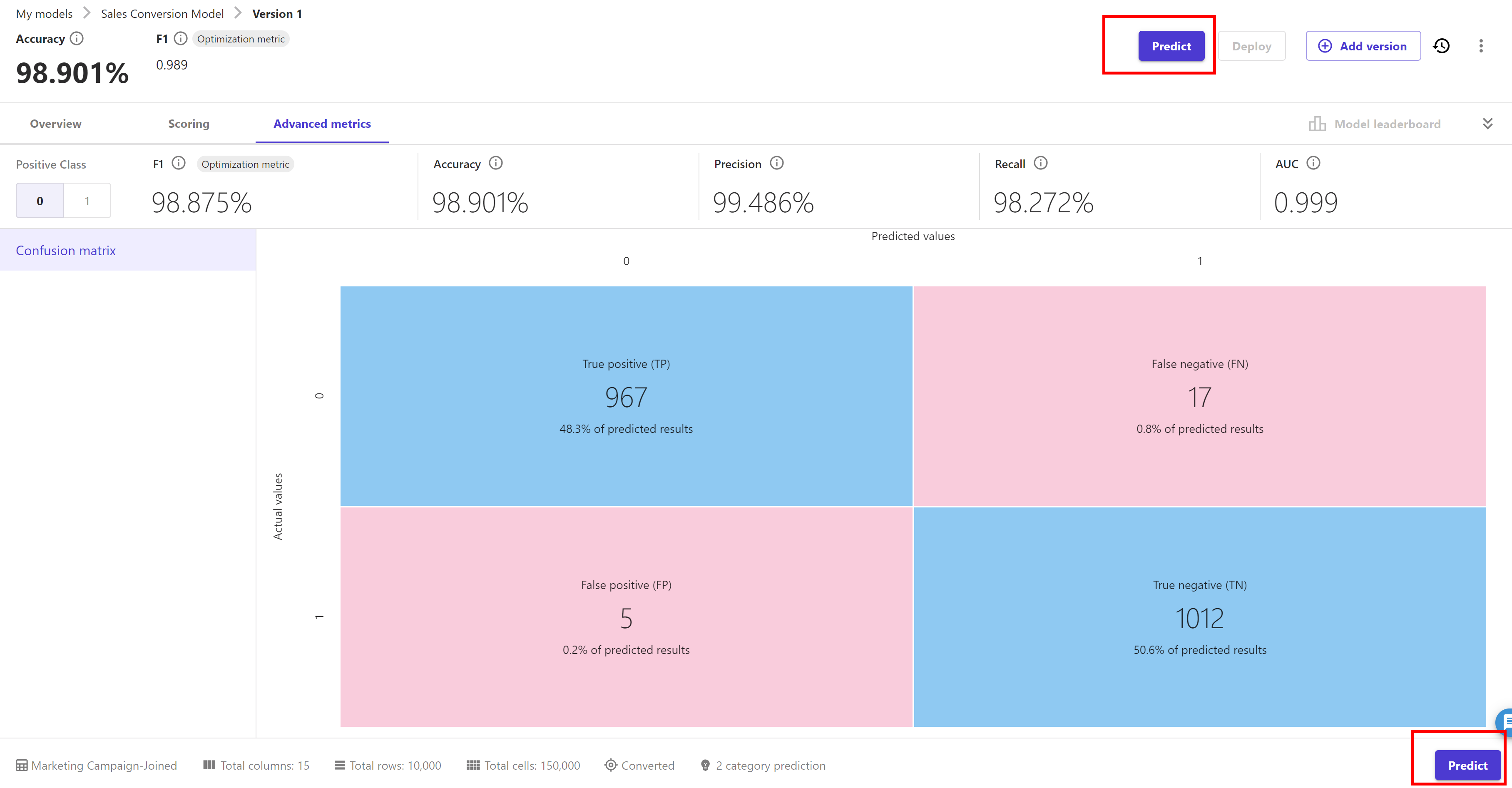
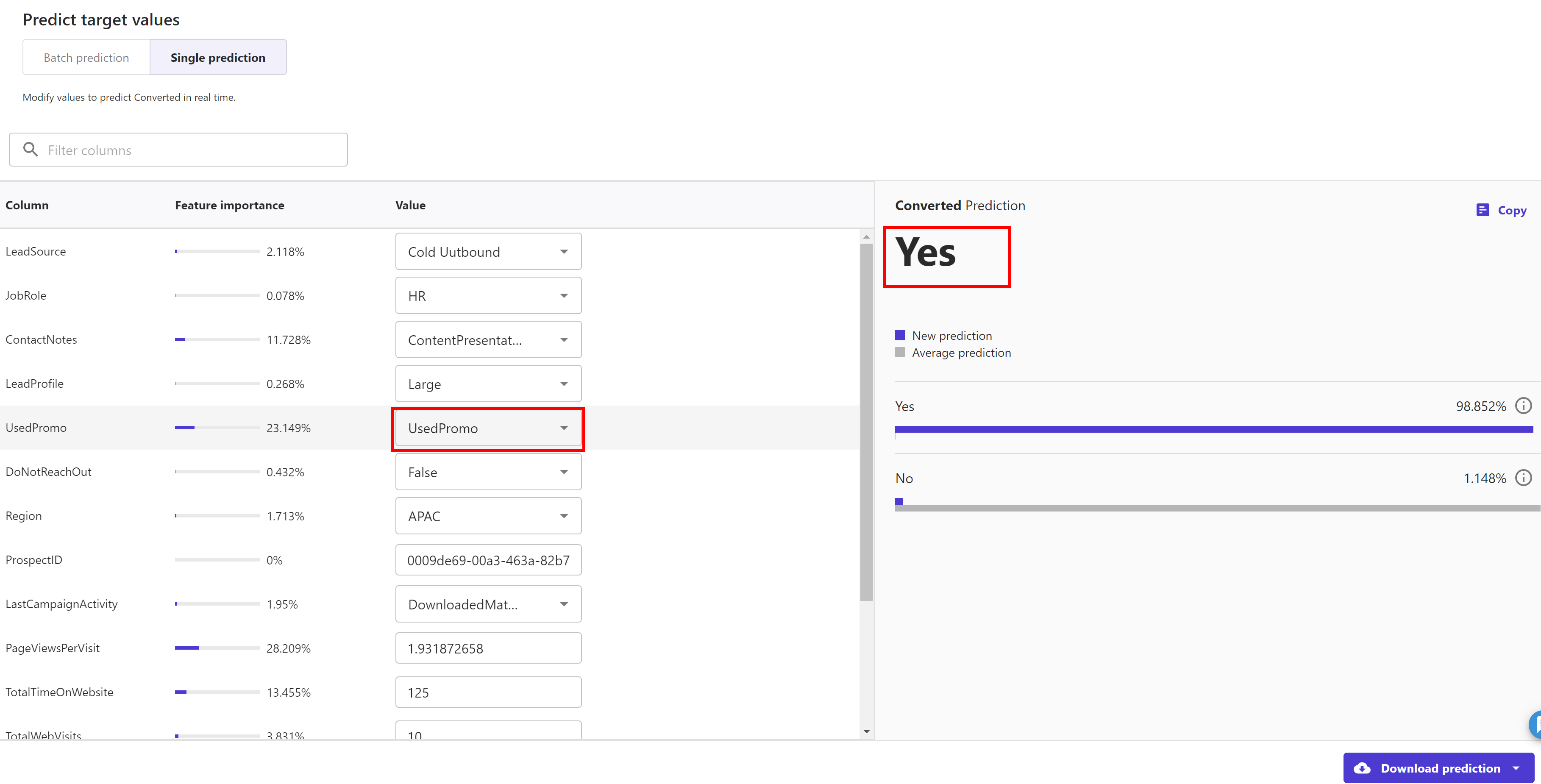
We can do a single prediction or batch prediction using Sagemaker Canvas. We do a single prediction here. click on the "Predict" button and then select "Single Prediction" tab. Sagemaker canvas automatically generates a sample data and predicts the target feature ( converted ) for this data. As you can see here, it predicted "No" as converted target feature for this sample data.
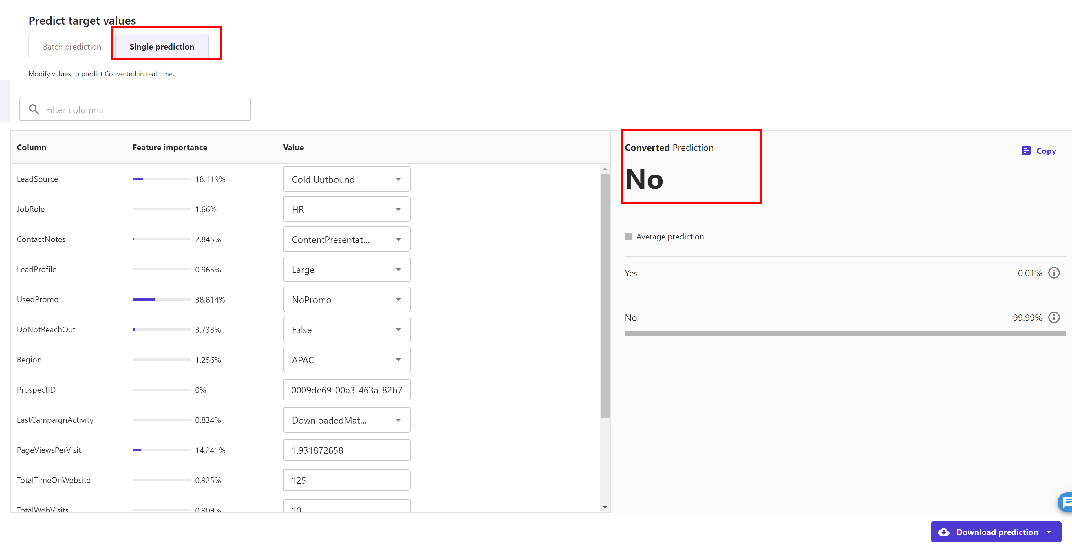
We can play around with this sample data and update the prediction after changing the data.
For example I changed "Usedpromo" from "NoPromo" to "UsedPromo"and hit the update button to predict the target feature again. This time it predicted "Yes" as converted target feature for this changed sample data.
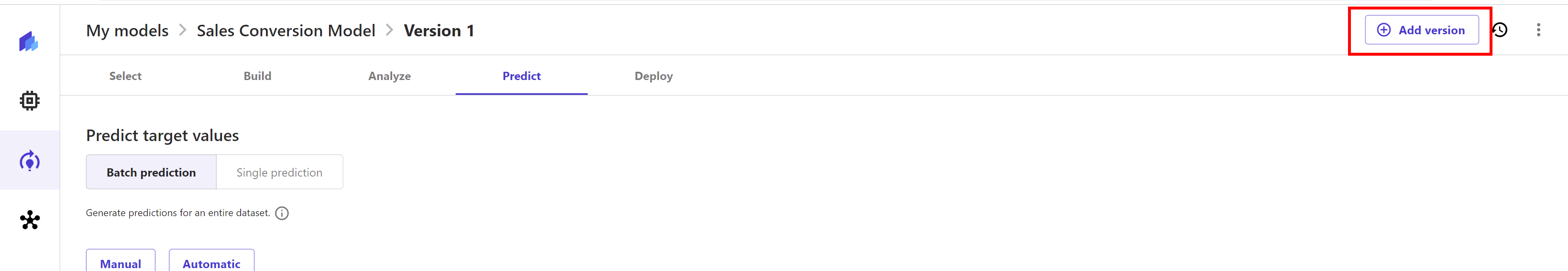
SageMaker Canvas supports building multiple version of a model. Now we create a new version of the above model but this time we train it using the "Standard build" option.
Click on the "Add version" button and it will create a V2 ( in draft status ) of this model:
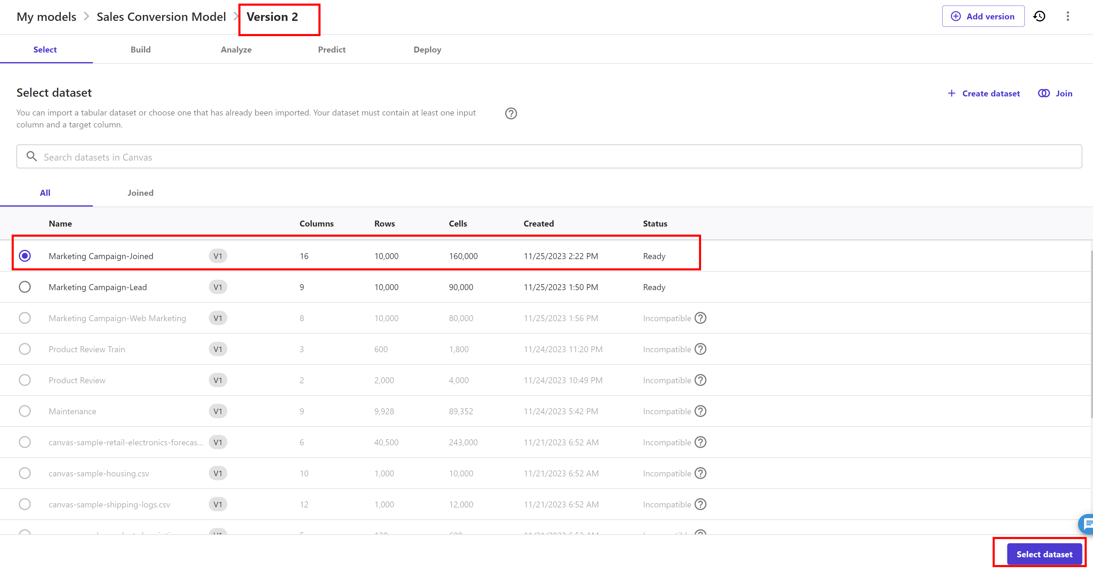
Now our model switch to Version 2. Below screen appears. Now, In the Select dataset page, select the our Marketing Campaign-Joined dataset and click Select dataset
Now build model screen appear ( like shown below ) and de-select the "ProspectID" feature as shown below ( as we don’t want to train our model with this feature ):
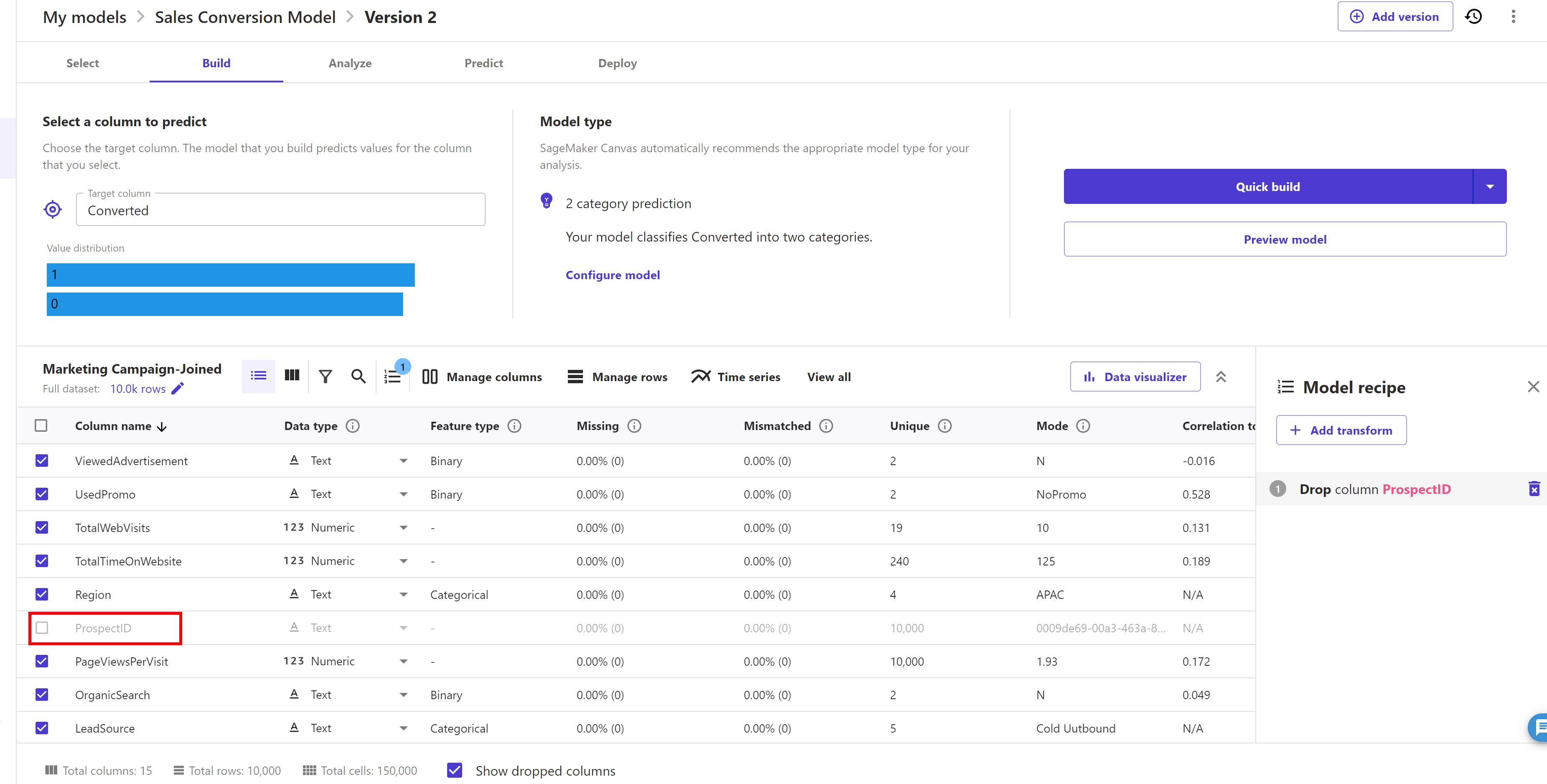
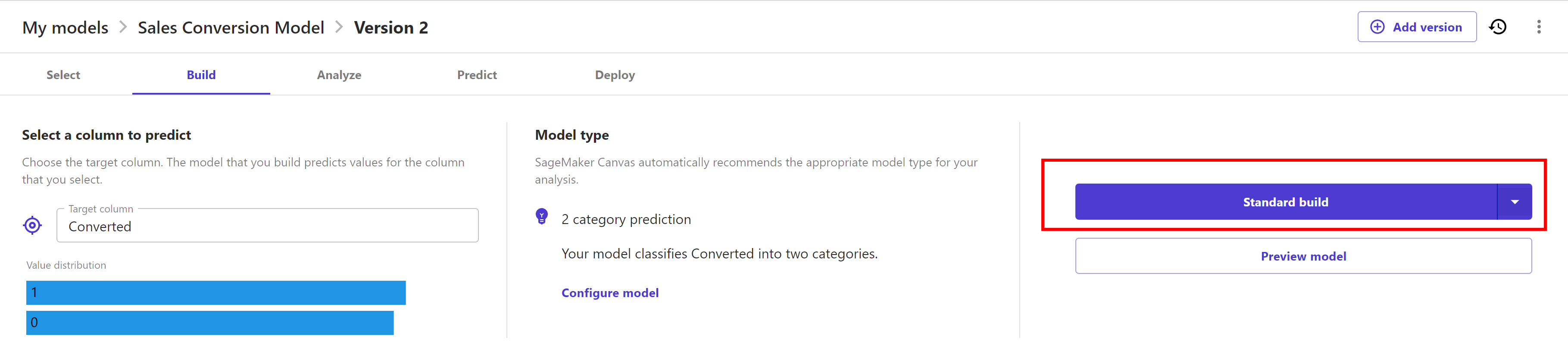
Now click on the dropdown of "Quick build" button and select "Standard build" option. Now click on "Standard build" button:
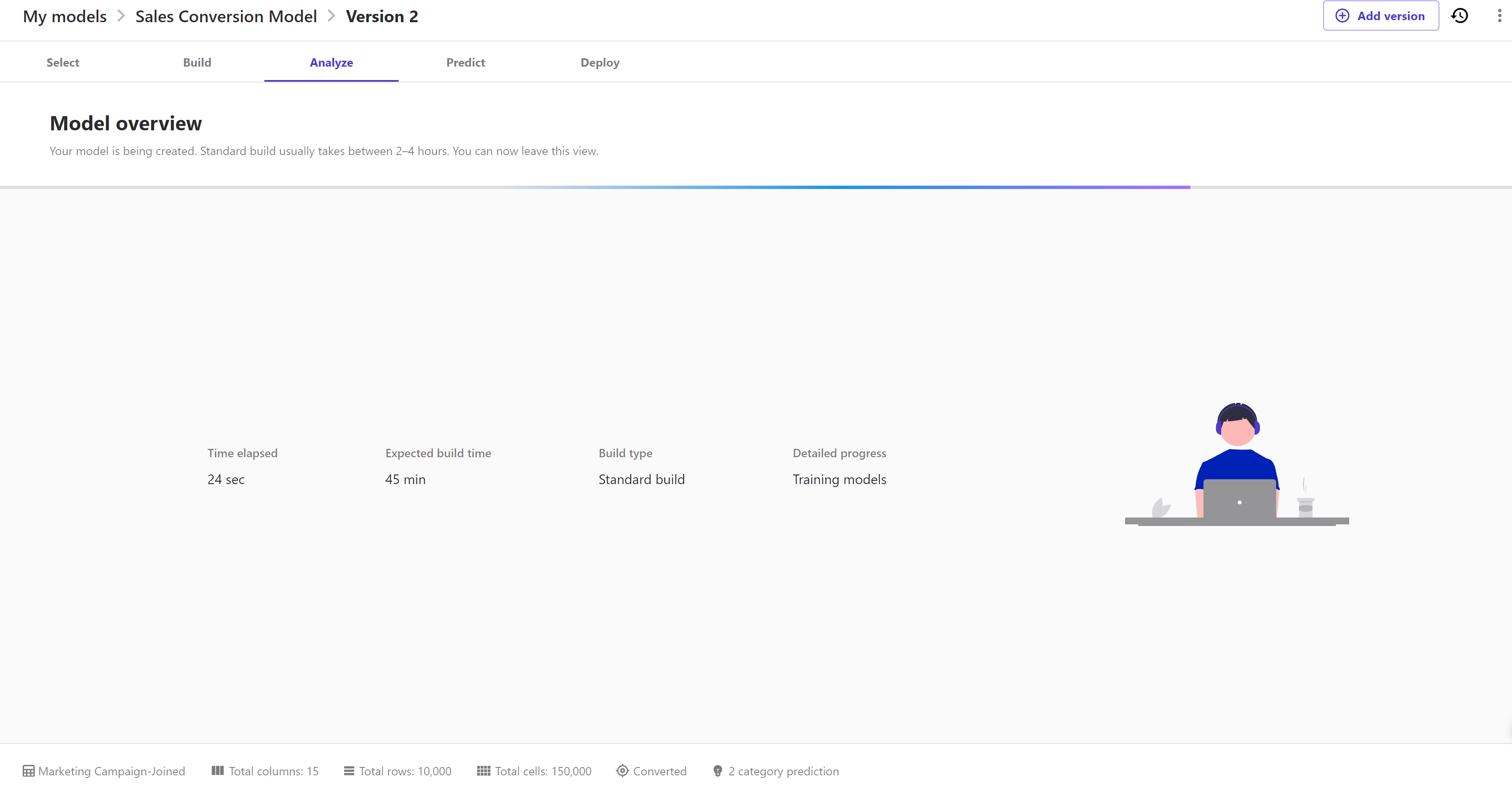
Now wait for model build completion as it will take around 45 minutes or less:
Once the model build is complete, it will jump to the "Analyze" page with the accuracy score and column impact by default.
Evaluate this model same as the previous model; by navigating to "Scoring" and "Advance Metrics" tabs. You can use this model to do either batch prediction or single prediction as well.