

Figure 1. Q-View Software workflow.
Q-View™ Software is a tool for the quantitative analysis of multiplexed
chemiluminescent planar-based arrays. Analysis is performed in three
easy steps (Figure 1) which are covered in detail in this manual:
-
Image Processing: Capture or import images, and align the plate overlay.
-
Well Assignment: Group, name, and apply dilution factors to wells.
-
Data Analysis: Customize and export concentrations, statistics, and charts.
-
Q-Plex™:
The brand name of the multiplex ELISA kits manufactured by Quansys Biosciences.
-
Q-View™ Imager LS:
The brand name of the life science chemiluminescent imager produced by Quansys Biosciences.
-
Q-View™ Imager Pro:
The brand name of the first clinical-grade chemiluminescent imager produced by Quansys Biosciences.
-
Q-View™ Imager Plus:
The brand name of the latest clinical-grade chemiluminescent imager produced by Quansys Biosciences.
-
Q-View™ Software:
The brand name of the multiplex ELISA analysis software produced by Quansys Biosciences.
-
Project:
A file with the ".Q-View" extension. Projects contain images, plate overlays, well assignments, and data
for one or more plates.
-
Plate Overlay:
The well diagram of the plate that is aligned by the user over the plate image comprising the spots within the well.
-
In-Kit Certificate of Analysis:
An In-Kit Certificate of Analysis is included with every Q-Plex kit. This card includes information such as the software product code,
the calibrator lot number, and the calibrator and/or control reconstitution volumes. It also includes a table of the analytes tested by the kit,
the associated calibrator concentrations, and a graphical representation of the spotted array.
-
Software Product Code:
The alphanumeric code that defines parameters such as the number and position of the spots in each well, the concentration
of each analyte in the calibrator, the optimal curve fit settings, and control ranges when applicable.
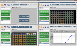
Figure 2. Multiple projects opened.
Q-View Software stores the images and analyses of related plates together in
a file, called a project, with the ".Q-View" extension.
As you work, changes to these projects are saved automatically.
Multiple projects can be open at the same time (Figure 2).
Before version 3.1, projects were stored as folders. Project folders can still be opened by the software but they will
be upgraded to the project file format when opened. Project files are specific to Q-View Software
and cannot be viewed or manipulated by 3rd party software.
Project details can be accessed by opening
Project > Project Details. The project creator, creation date, and a list of
users that have opened the project along with associated timestamps are recorded.
Project notes can be recorded and viewed by opening
Project > Project Notes. These notes allow users to record
read-only messages related to the project.
Whenever a project is closed or a report is exported, the full report is recorded if it has changed in any way.
Project history can be viewed by opening
Project > Project History.
Projects saved on a network need to be accessed through mapped network drives (e.g. Z:\myProject.Q-View) and not network locations (e.g. \\server\myProject.Q-View).
-
Installation
-
Install Q-View Software on any number of computers.
-
Set up your imager and any other equipment to be used for the experiment.
-
Using a Q-View imager, ensure the imager has been focused, dark field images
have been captured, and set-up is complete before proceeding. All of these procedures can be found in the
Q-View Imager LS, Pro, and Plus manuals.
-
Process and image the Q-Plex kit
-
Process the Q-Plex kit according to the instructions in the kit manual.
-
Capture the image(s) using a Q-View imager or other compatible, third-party imager.
With third-party imagers, only grayscale, TIFF and CR2 image files of at least 12 bits per pixel should
be imported for scientific reporting purposes. Images with a white background must be inverted within Q-View Software by clicking
Image Options > Invert Image
.
-
Analyze images in Q-View Software
-
Enter the software product code
(found on the In-Kit Certificate of Analysis) for each plate.
-
Within Image Processing, set the plate overlay.
-
Perform Well Assignment.
-
Within Data Analysis, click Perform Analysis to generate
charts and reports. Customize and export the results as desired.
-
Ensure the computer meets the following minimum specification:
-
Windows® 10 or 11
Note: The Windows® version of the Q-View Software is required to operate Q-View imagers. The Mac® operating system is not compatible with Q-View imagers.
-
Mac® OS 10.15 or newer
-
4 processing cores
-
8 GB RAM
-
USB 2.0 (Type A) or greater for Imager LS and Imager Pro. USB 3.0 (Type A) or greater for Imager Plus. USB C is not supported.
-
Screen resolution of 1280x800 or greater
For optimal performance:
-
16+ GB RAM
-
8 or more processing cores
-
If you do not have a Q-View Software installer, contact a Quansys Biosciences representative by email
at sales@quansysbio.com
or call 1-888-782-6797.
-
Launch Q-View Software. Click either Evaluate Q-View
to start a 60 day trial or enter your assigned company name and
license key and then click Continue. Follow the prompts on
the screen to set up user accounts and Q-View imagers. You
can change these settings later from the
Settings menu.

Figure 3. USB and power sockets.
- Carefully unpack the Q-View imager and place it on a clean work area.
- Plug the power cord into the back of the imager (Figure 3) and into a surge protector.
-
Plug the USB cord into the back of the imager (Figure 3) and into the computer. For the Q-View Imager Pro and the Q-View Imager Plus,
ensure the power switch is in the on position. The Q-View Imager Plus requires USB 3.0 or greater.
- Clean the tray glass with a lint-free cloth and ethanol, rubbing alcohol, or window cleaner.
-
Launch Q-View Software and open Settings > Manage Imagers to discover, name, and focus the
imager and to capture a dark field. Dark field capture takes approximately 15 minutes on the Q-View Imager LS and the Q-View Imager Pro, and 35 minutes on the Q-View Imager Plus.
-
The Q-View Imager Pro requires drivers that are not bundled with the Q-View Software installer.
Please contact Quansys Biosciences to obtain and install these additional drivers if needed.
-
The button on the front of the Q-View Imager Pro opens and closes the tray. Its color represents the following.
- Green: the imager is on and the tray can be opened
- Red: the tray is open
- Yellow: images are being acquired and the tray is locked
- Flashing Red: the imager is alerting the user to an abnormal condition
-
Q-View Software turns the imager on after it is detected and turns it off when the application closes.
-
The sensor is cooled to deliver highly reproducible imaging. Cooling will be turned off
after one to four hours of inactivity based on your preference. Cooling will be turned back on when
image capture begins or sooner if the Activate Now link is clicked.
-
If the sensor is not at the optimal temperature when the user attempts to capture an image, image capture will
be postponed until the temperature target has been reached (generally about one minute).
-
Keep the cooling vents on the bottom, sides, and back clear of debris. If the vents are obstructed
the imager may overheat. When overheated, the sensor's cooler will be turned off, the open/close button will
flash red, and image capture will be prevented.
-
The Q-View Imager Plus requires drivers that are not bundled with the Q-View Software installer.
Please contact Quansys Biosciences to obtain and install these additional drivers if needed.
-
The button on the front of the Q-View Imager Plus opens and closes the tray.
-
The LED light on the front of the Q-View Imager Plus will change color to indicate the status of the device.
The indicator color scheme has been designed to be user friendly for those with normal vision and common forms of color blindness.
The table below is the legend for status light indication.
| LED Color | Activity | Imager Status |
|---|
| White | Solid | Startup |
| White | Pulse | Sleep |
| White | Strobe | Firmware update |
| Magenta | Solid | Idle, software not connected |
| Blue-green | Solid | Idle, software connected |
| Yellow | Solid | Tray in motion or open |
| Yellow | Strobe | Tray obstruction |
| Blue | Solid | Plate imaging |
| Blue | Pulse | Imaging with internal lights |
| Red | Solid | Fatal error |
Activity Definitions
- Solid: Constant with no flashing or dimming
- Pulse: Slow dimming and brightening
- Strobe: Rapid flashing
If 'fatal error' occurs, contact the manufacturer for support.
-
The sensors are cooled to deliver highly reproducible imaging. Cooling will be turned off
after five minutes of inactivity. Cooling will be turned back on when image capture begins or sooner if the Activate Now link is clicked.
-
If the sensors are not at the optimal temperature when the user attempts to capture an image, image capture will
be postponed until the temperature target has been reached (generally about one minute).
-
Keep the cooling vent on the bottom and back clear of debris. If the vents are obstructed
the imager may overheat. When overheated, image capture will be prevented.
-
The Q-View Imager Plus is designed to operature within an ambient temperature range of 15°C (59°F) to 27°C (80°F).
If the ambient temperature falls outside of this range, sensor cooling may be affected and imaging may be unavailable.
-
The Q-View Imager Plus is focused during manufacturing and is not user-focusable.
-
The Q-View Imager Plus comes equiped with a barcode scanner. Q-View's barcode catalog needs to be kept up-to-date
for the scanner to read your plate's product code. See Software and Product Updates for details.
-
When importing archived images captured by a Q-View Imager Plus, Q-View needs to be connected to the imager and all four images need to be imported at the same time. This will allow the images to processed and combined into a single image as opposed to importing four distinct, unprocessed images.
-
USB 3.0 (Type A) or higher is required. The imager will not connect when plugged into USB 1 or USB 2. USB Type C to Type A conversion is also not supported.
When user accounts are enabled, users are required to log in to use the software.
Administrators can manage users during software setup or by opening
Settings > Administration > User Accounts (Figure 4).
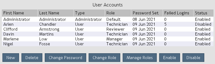
Figure 4. User accounts.
-
New: Create a new user.
-
Delete: Delete the selected user(s).
-
Rename: Rename the selected user.
-
Change Password: Set the password of the selected user(s).
-
Change Role: Set the role of the selected user(s).
-
Manage Roles: Open user role management.
-
Enable: Enable the selected user(s). Enabled users can log in.
-
Disable: Disable the selected user(s). Disabled users cannot log in.
Administrators can set their organization's password policy by opening
Settings > Administration > Password Policy (Figure 5).
The password policy defines the following password requirements:
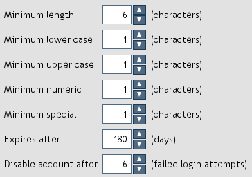
Figure 5. Password policy.
-
Minimum length: The minimum number of characters.
-
Minimum lower case: The minimum number of lower case characters.
-
Minimum upper case: The minimum number of upper case characters.
-
Minimum numeric: The minimum number of numeric characters.
-
Minimum special: The minimum number of special characters.
-
Expires after: The number of days from the day the password was set until the password expires.
When a user's password expires, the user will be forced to set a new password at the next successful login.
-
Disable account after: The number of failed login attempts before the user account is disabled.
When a user account is disabled, the user is prevented from logging in until an administrator enables the account.
When set to zero, there is no limit to the number of failed login attempts.
Administrators can manage user roles by opening
Settings > Administration > User Roles (Figure 6).
User roles define permissions which allow or disallow users from accessing various software features.
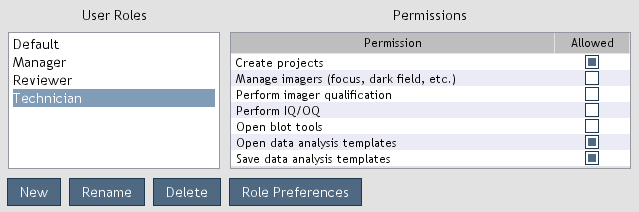
Figure 6. User roles and associated permissions.
By default, users are assigned the
Default role which allows all permissions.
The default role permissions cannot be modified. Users can view their permissions by opening
Settings > Permissions (Figure 7).
-
New: Create a new user role.
-
Rename: Change the name of the selected user role.
-
Delete: Delete the selected user role.
-
Role Preferences: Set preferences that are applied to the users assigned to the role.
Permissions are granted by selecting the
Allowed check box adjacent to the permission (Figure 6). Permissions are revoked by deselecting the check box.
The permissions are described as follows:
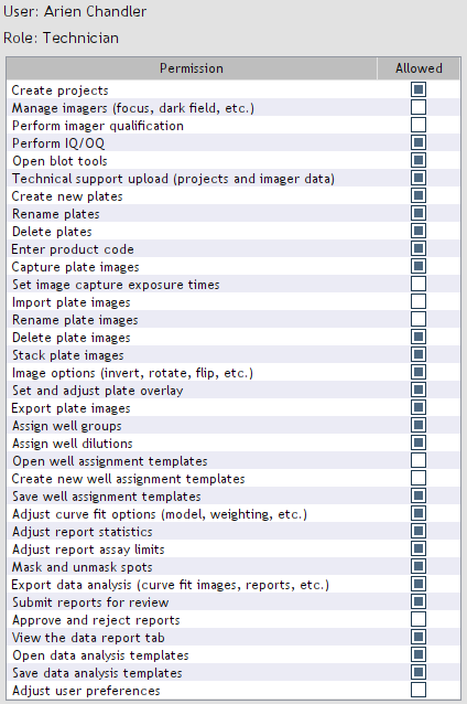
Figure 7. User permissions.
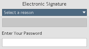
Figure 8. Electronic signature.
When documents are saved, electronic signatures (Figure 8) are required if user accounts are enabled.
The name of the signee, a reason for the signature, and a timestamp are appended to the document.
Electronic signatures apply to the following:
-
Well assignment templates: When a well assignment template is saved, an electronic signature is required. The template file is encrypted to prevent modification.
-
Data analysis templates: When a data analysis template is saved, an electronic signature is required. The template file is encrypted to prevent modification.
-
Report review submission: When a report is submitted for review, an electronic signature is required.
-
Report approval: When a report is approved, an electronic signature is required.
-
Report rejection: When a report is rejected, an electronic signature is required.
-
Report exporting: When a report is exported, an electronic signature is required. The signatures are found at the bottom of the exported CSV file.
-
Application settings: When settings are exported, an electronic signature is required. The settings file is encrypted to prevent modification.
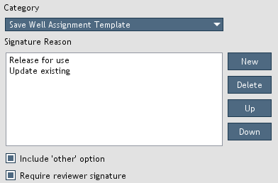
Figure 9. Electronic signature settings.
Electronic signature settings (Figure 9) can be accessed by opening
Settings > Administration > Electronic Signature Settings. You can create or delete signature reasons for specific categories.
The order of the reasons can by modified by moving them up or down in the list.
When the
Include 'other' option is selected, an 'other' option will be included in the reason drop-down list (Figure 8).
A free-form text field will be enabled allowing the user to enter a custom reason.
When the
Require reviewer signature option is selected, exporting reports requires that they first be submitted for review by users with the
Submit reports for review
permission and subsequently approved by users with the
Approve and reject reports permission.
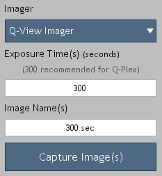
Figure 10. Image acquisition options.
-
Place the plate in the Q-View imager and close the lid/tray. Select the desired imager and enter the exposure time(s) and image name(s) (Figure 10). If the desired imager is not listed, select Refresh from the drop-down to scan for imagers.
The recommended exposure settings for Q-Plex kits are:
-
Q-View Imager LS: 270 seconds
-
Q-View Imager Pro: 300 seconds
-
Q-View Imager Plus: 300 seconds
-
Capture the image(s) by clicking Capture Image(s).
You can continue to Well Assignment while images are being captured.
-
Add a plate tab for each physical plate to be imaged by clicking
the + tab (Figure 11). Custom plate names can be set by double clicking the plate name.

Figure 11. Plates organized by tabs.
Note: The Enable Internal Illumination option is available for Q-View Imager Pro models when activated in Settings > Preferences.
When enabled, the imager's internal focus lights are turned on during image acquisition. This may be useful for quality control
but should not be enabled when capturing Q-Plex images.
Before importing an image, ensure it is grayscale and has a pixel
depth of at least 12 bits. Q-View Software can open TIFF, CR2, BMP, PNG, and JPEG files.
Low bit depth and lossy images (BMP, PNG, and JPEG) are insufficient
for analysis and should be imported for display purposes only.
To import an image, click Image Processing > Import Image
or drag and drop image files onto the list of images.
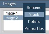
Figure 12. Image pop-up menu.
Images can be renamed, deleted, or stacked by right-clicking an image
name (Figure 12). Image details can be viewed by selecting properties.
Click
Export to save an image as a lossless TIFF or compressed JPEG.
JPEG files are suitable for display purposes only and should not be used for analysis.
-
Enter the Software Product Code from the In-Kit Certificate of Analysis
into the Product Code field.
-
Use Image Options to adjust image gamma, zoom, and orientation as desired.
Images with black spots on a white background need to be
inverted by clicking Image Options > Invert Image.
-
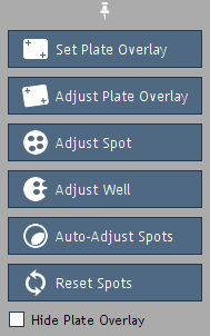
Figure 13. Overlay Options.
If you are using the Auto-Set Plate Overlay
feature, the initial overlay position will be set
automatically. Otherwise, click Overlay Options > Set Plate Overlay,
and click and drag the mouse cursor from the center of the top-left
well to the center of the bottom-right well. Use the following
Overlay Options (Figure 13), if needed, to manually adjust the overlay:
-
Set Plate Overlay:
Set the plate overlay by dragging from the center of the top-left well to the center of the bottom-right well.
-
Adjust Plate Overlay:
Pivot or expand/contract the entire overlay via clicking
and dragging the corner wells highlighted in blue.
-
Adjust Spot and
Adjust Well:
Click and drag to move either an individual spot in
the overlay, or all spots in a well. Use the keyboard arrow keys for more precise adjustments.
-
Auto-Adjust Spots: Automatically adjusts all spots to improve the alignment of the overlay.
-
Reset Spots: Reset all spots in the overlay to
their default locations.
-
Hide Plate Overlay:
View the image without the plate overlay.
When using a Q-View imager, the
Auto-Set Plate Overlay
feature, found in
Settings > Preferences,
can be enabled to cause the software to provide the initial plate overlay position.
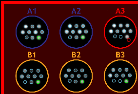
Figure 14. Plate overlay.
This feature is activated after manually setting a plate overlay for
the first time. Once activated, the
Auto-Set Plate Overlay
feature will automatically set the overlay onto all
captured
images as soon as the product code is entered.
Be sure to review the accuracy of the overlay placement for each captured image.
When using a Q-View Imager LS, Q-View Imager Pro, or Q-View Imager Plus with Q-Plex plates, Auto Spot Finding will be active and will
make it easier to accurately set the plate overlay either manually or via the Auto-Set Plate Overlay feature.
For products with defined assay controls, the assay control spots that are in range are outlined in green.
Spot(s) and associated well(s) that are out of range are outlined in red (Figure 14).
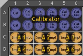
Figure 15. Well assignment.
Assign well types, names, and dilution factors in either Q-View Software or
a spreadsheet application such as Microsoft Excel. Use
Well Assignment Templates to quickly assign repeat layouts.
To assign well types and names, select the desired wells by clicking and dragging the mouse over the plate image (Figure 15).
Hold the control key to select discontiguous groups of wells.
Click
Groups (Figure 16) and enter custom names if desired.
Select one of the well types defined below to register the assignment.
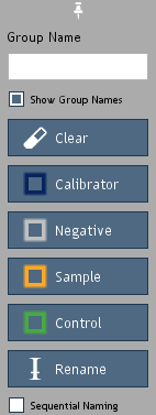
Figure 16. Group tools.
-
Calibrator: The kit calibrator (antigen standard).
-
Negative: The calibrator curve negative (blank) where only sample
diluent was loaded.
-
Sample: The biological sample (unknown) being tested.
-
Control: User positive control samples. The known
concentrations of these samples may be predefined by Quansys Biosciences with an
acceptable range. If an analyte in a predefined control fails to meet the criteria, an error code will be
included in the report tab of Data Analysis.
-
Rename: Rename well groups without modifying well type.
Calibrators may be assigned dilution factors or grouped by predefined concentrations for each analyte.
Predefined concentrations are created by Quansys Biosciences and assigned by the user by selecting a well group,
clicking the
Calibrator button (Figure 16) and then choosing from a list of group names in a subsequent pop-up window.
Use
Sequential Naming to automatically name groups of wells with sequentially increasing suffixes.
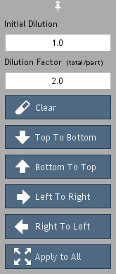
Figure 17. Dilution tools.
To assign dilution factors (Figure 17), select the desired wells and click the
Dilutions button. Enter the dilution factor
of the initial dilution in the
Initial Dilution field. For example,
enter the number "2" for a 1:2 (50%) dilution. If a dilution
series was continued from that initial dilution, enter the series dilution
factor. For example, to indicate a 1:10 dilution series from the
1:2 (e.g. 1:20, 1:200, 1:2000), enter "10" in the
Dilution Factor field.
Press any of the directional buttons, e.g.
Top to Bottom,
to register the assignment.
To assign well types, names, and dilutions in spreadsheet software
such as Microsoft Excel, click Templates > New Template,
then name and save the newly created template file. Once saved, a
blank well assignment template will open in the default spreadsheet
software. Fill this out and save your changes. Apply the template
as described below.
To save your current well assignment as a template, click
Templates > Save Template. To apply a
previously saved template to a plate, either click
Templates > Open Template, or drag and drop
the template file onto the plate diagram.
Once you have completed
Image Processing and
Well Assignment, select
Data Analysis. Click
Perform Analysis to generate charts,
concentrations, and statistics based on optimal regression settings provided
by the product definition. Click the
Curve Fit Options button
to customize regression models, weighting, and negative well subtraction settings.
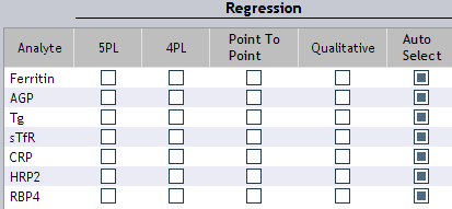
Figure 18. Curve fit regression options.
The default 4PL or 5PL regression models are generally recommended
for most Q-Plex data, as these are widely considered to provide
the best overall fit for immunoassay curves. If your data is abnormal
or you are trying to optimize the fit for a particular range, one of
the other regression models, along with masking, may better fit your
needs. You can choose from the following
Curve Fit Options (Figure 18):
Regression Models
-
5 Parameter Logistic (5PL):
This non-linear regression model is generally considered the
best for fitting sigmoidal immunoassay calibrator curves and
is recommended for Q-Plex kits.
-
4 Parameter Logistic (4PL):
This non-linear regression model, which is slightly less complex
than 5PL, is also considered an acceptable model for analyzing
ELISA calibrator curves, particularly if the calibrator curve is
symmetric.
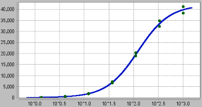
Figure 19. Example 5 Parameter Logistic chart.
-
Point to Point:
Also known as spline analysis, unknowns are determined by
straight lines between each calibrator point in this regression model.
-
Qualitative:
This option is for kits that do not come with a calibrator; no
concentrations are calculated. Bar charts show the average
pixel intensity for each well group and dilution.
-
Auto Select:
This option selects the best regression model and weighting
for each assay by fitting and comparing all regression models.
In products with spot replicates, replicates within each well are
averaged and treated as single data points. Calibrator curves for assays
with spot replicates are fit to the replicate average using the specified
regression model.
Calibrator curves for our High Dynamic Range Singleplex assays are
automatically fit using the HDR algorithm irrespective of the chosen
curve fit option.

Figure 20. Curve fit negative subtraction and weighting options.
Weighting
Weighting options are available after selecting
Show Advanced Options.
Weighting is used to reduce the impact of outliers and offset heteroscedasticity. In ELISA calibrator curves, the residuals (variability) tend to increase as the concentration of the calibrator (y) increases.
To improve curve fit, various weighting methods can be applied. General weighting (y) can be applied to normalize the residuals across the curve based on the signal of each calibrator point.
Weighting based on residuals (r), reduces the impact of outliers on the curve fit. The larger the number associated with either weighting method, the more variation there will be between the impact of the calibrator points on the final curve fit.
Curve fit can be evaluated by looking at the percent backfit value in the report. When samples fall at the low or high end of the curve, goodness of fit should be prioritized at that end of the curve.
Selecting
Favor Low or
Favor High evaluates the percent backfit across the curve and will automatically select the weighting method that results in the best fit for either the low or high end of the curve.
Negative Well Subtraction
Negative well subtraction (Figure 20) automatically deducts the average signal (pixel intensity)
of the negative wells from the signal of all other wells for each analyte.
Curve fit and calculated concentrations are not affected by negative well subtraction.
The default state, on or off, can be changed in
Settings > Preferences.
Concentrations, pixel intensities, and statistics are displayed
based on the selected
Data Analysis tab (Figure 21), spot masking, and
settings in the
Statistics and
Assay Limits menus.
Results are organized into three tabs for each plate:
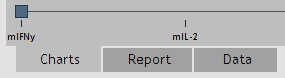
Figure 21. Data Analysis tabs.
-
Charts Tab:
Displays the regression model charts for quantitative assays,
or bar graphs for qualitative assays. The selected regression model and weighting
are included above each chart when enabled (Statistics >
Assay > Show Regression Model). Hover the mouse
over a point to view (x, y) values. Right-click to access
masking options and chart properties. Click and drag from
top-left to bottom-right to zoom in. Click and drag from
bottom-right to top-left to zoom out.
-
Report Tab:
Displays concentrations and other calculations based on settings
in the Statistics and Assay Limits menus.
-
Data Tab:
Displays concentrations or pixel intensity values based on settings
in the Statistics and Assay Limits menus.
Other values that may appear in the
Report and
Data tabs are:
-
Incalculable (High/Low):
The concentration could not be calculated typically because it fell
either above or below the parameters of the curve. The reported value
can be customized in Settings > Preferences.
-
NA:
Not Applicable. Note that certain statistics cannot be calculated
if there is only one replicate present or there are no
negative wells assigned.
-
No Fit:
The curve did not fit using the selected curve fit settings.
-
Empty:
No well assignment was provided by the user for the well.
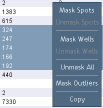
Figure 22. Masking spots.
Select and right-click (Figure 22) data points within the
Chart,
Report or
Data tab to mask (exclude from all calculations)
or unmask spots and wells.
Q-View Software can automatically identify and mask outliers in calibrator curve data. To enable this feature,
open
Settings > Preferences and select
mask calibrator outliers by default. When you unmasked an auto-masked outlier,
Q-View Software will not auto-mask the point again when fitting curves until you right click a chart or report and select
Mask Outliers
(Figure 22) from the drop-down menu.
Click
Statistics (Figure 23) to select which calculations are shown.
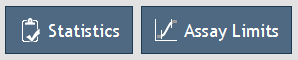
Figure 23. Statistics and Assay Limits.
If multiple dilutions of a sample were present, select
Auto-Select Dilution to view only the data for the dilution
that fell on the most linear part of the calibrator curve, instead
of data for every dilution of the sample.
Click
Assay Limits (Figure 23) to modify how extrapolated data is displayed:
-
ULOQ and LLOQ – Upper and Lower Limits of Quantification:
These are the average of the highest/lowest calibrator points
with a %backfit of 120%-80%, a %CV of <30%, and a positive
mean pixel intensity difference between the calibrator point and
the negative control. These are the recommended upper and lower range limits, allowing concentrations
only for data within the quantifiable range of the calibrator curve
(interpolated) to be displayed.
-
LLD – Lower Limit of Detection: The lower limit can
alternately be set to the LLD to view
concentrations down to this value. LLD is the lowest concentration
of analyte that can be reliably distinguished from background noise.
Note that values below the LLOQ are extrapolated.
-
LOB - Limit of Blank: The lower limit can alternately be
set to the LOB to view concentrations down to this value.
LOB is the expected signal when measuring samples that contain no analyte.
Note that values below the LLOQ are extrapolated.
-
LOD - Limit of Detection: The lowest concentration of analyte
that can be reliably distinguished from the LOB with a defined level of statistical confidence.
-
Lot LLD, LLOQ, or ULOQ:
The Lot limits, only available for certain products,
are the assigned Lot LLD, LLOQ and ULOQ values determined by Quansys Biosciences.
-
No Limit:
Q-View Software will display concentrations for all points that can
be calculated with the chosen regression model, including
those extrapolated below the LLOQ and the LLD.
Backfitting of the calibrator is a practical method for evaluating the quality of the curve fit.
This is done by comparing the calculated concentration of each calibrator to its known (theoretical)
concentration using the equation: calculated concentration / theoretical concentration x 100%. Q-View Software
displays this result in the report as percent backfit. The preferred result for each calibrator
point is a backfit value of 80%-120%, although 70%-130% may be acceptable.
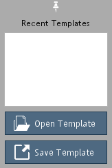
Figure 24. Data analysis templates.
Custom curve fit settings, statistics and assay limits can be saved in the Data Analysis Templates section (Figure 24).
To save your current settings as a template, click Save Template.
To apply a saved template, click Open Template or drag
and drop a template file onto the data analysis section.
The error code column in the report alerts you to potential problems with your assay.
Error codes are defined at the bottom of the report and include:
-
Assay Controls (AC): Within a product, analytes may be designated as assay controls and assigned an acceptable range of pixel intensity values. This error is raised when an analyte’s measured pixel intensity falls outside its defined range.
-
Process Controls (PC): When a product includes a process control, users must select a process control during well assignment. The selected control determines the well group name and specifies acceptable concentration ranges for associated analytes. This error is raised when an analyte’s calculated concentration is outside the defined range.
-
Spot Overlay Out of Bounds (SB): This error is raised if any wells in the plate overlay overlap one another, or if any individual spots fall outside the defined boundaries of their respective wells.
-
Pixel Intensity Coefficient of Variation (CV): This error is raised when the coefficient of variation (CV) between a sample and its corresponding control exceeds 30%.
-
Masked Outliers (MO): This error is raised when one or more spots are automatically identified as statistical outliers and subsequently masked during analysis.
When
User Accounts are enabled and the
Require reviewer signature
option is selected, reports are required to be submitted for review (Figure 25) and subsequently approved before they can be exported. Users are required to have the

Figure 25. Submit for review.
Submit reports for review permission to perform this action. If a report changes after it has been submitted for review,
resubmission for review is required. This does not apply if the user who modifies the report has the
Approve and reject reports permission.

Figure 26. Review report.
Users with the
Approve and reject reports permission can approve or reject reports (Figure 26) submitted for review.
Rejected reports must be resubmitted for review and approved before they can be exported. Approved reports can be exported by users who have the
Export data analysis permission.

Figure 27. Export.
Click Export (Figure 27) to save charts as images, or the currently displayed values in the Report or Data tabs as a spreadsheet (CSV).
To qualify imagers, light is measured at constant intensities across the dynamic range
of the imager and compared to expected values. Quansys Biosciences supplies two
qualification plates; one for Q-View Imager LS and Q-View Imager Pro and another for Q-View Imager Plus.
Performing qualification on a regular basis ensures that the imager consistently meets performance specifications.

Figure 28. Q-View Imager Qualification menu.
Q-View Software imager qualification settings (Figure 29) can be accessed from the
Qualification > Q-View Imager Qualification > Settings menu (Figure 28).
The settings are accessible to only administrators.
-
Enable Q-View Imager Qualification: When enabled, image acquisition is restricted based on the qualification
settings and status.
-
Qualification Expiration: Defines the amount of time that an imager is considered qualified.
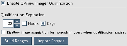
Figure 29. Q-View Imager Qualification settings.
-
Disallow image acquisition for non-admin users when qualification expires: When selected,
non-administrator users are not allowed to capture images when qualification expires (Figure 30).
-
Build Ranges: Builds qualification range parameters by processing a series of qualification plate images.
-
Import Ranges: Imports predefined ranges provided by Quansys Biosciences.
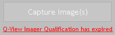
Figure 30. Image capture is restricted.
For Q-View Imager LS and Q-View Imager Pro, power on the
Q-View Qualification Plate and place it in the imager face down in the lower right corner of plate deck. For Q-View Imager Plus, place the
Q-View Qualification Plate in the imager with the barcode facing the rear.
Select
Qualification > Q-View Imager Qualification > Perform Qualification
from the menu (Figure 28) or click
Q-View Imager Qualification has expired (Figure 30) from the
Image Acquisition screen. Confirm that the serial number on the qualification plate matches the
serial number in the window. The process takes about 5 minutes to complete.
To view and export qualification reports, select Qualification > Q-View Imager Qualification > Reports (Figure 28) from the menu.
For Q-View Imager LS and Q-View Imager Pro, qualification plate certification expires annually. The expiration date is shown on the back of the plate. Once certification has expired, please contact Quansys Biosciences to arrange to have your plate recertified. Once your plate has been recertified and returned to you, it is necessary to rebuild the qualification ranges.
To build qualification ranges, open Qualification > Q-View Imager Qualification > Settings > Build Ranges and follow
the instructions provided by the software.
IQ/OQ is an add-on module that ensures the installation and operational functions of the imager and software are performing
correctly. These tests can be used upon initial evaluation and subsequent evaluations to ensure consistent operation of the Q-View imager and software.
Following the IQ/OQ testing, a report is generated that may be used for regulatory compliance and equipment control.

Figure 31. Imager & Software IQ/OQ menu.
Imager & Software IQ/OQ settings (Figure 32) can be accessed from the
Qualification > Imager & Software IQ/OQ > Settings menu (Figure 31).
The settings are accessible to only administrators.
-
Enable Imager & Software IQ/OQ: When enabled, image acquisition is restricted based on the qualification
settings and status.
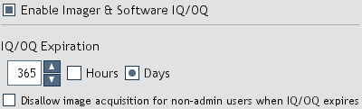
Figure 32. Imager & Software IQ/OQ settings.
-
IQ/OQ Expiration: Defines the amount of time qualification is considered valid.
-
Disallow image acquisition for non-admin users when IQ/OQ expires: When selected, non-administrator users
are not allowed to capture images when IQ/OQ expires (Figure 33).
In the Q-View Software, select
Qualification > Imager & Software IQ/OQ > Perform Qualification from the menu
(Figure 31) or click
Imager & Software IQ/OQ has expired (Figure 33) from the
Image Acquisition screen.
The process takes about 15 minutes to complete.
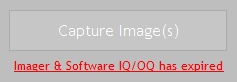
Figure 33. Image capture is restricted.
To view and export qualification reports, select Qualification > Imager & Software IQ/OQ > Reports (Figure 31) from the menu.
Click
Support > Legacy Blot Tools to make custom selections for western blots,
northern blots, southern blots, dot blots, and other chemiluminescent images.
Click
Close to return to the previous
Image Processing screen.
Click
Selection Options and choose one of the following tools
to make a custom selection (Figure 34).
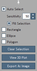
Figure 34. Blot tools.
Auto Select: Automatically select a group of similar, contiguous pixels by clicking on the center of the grouping.
The number of shades included in the selection correlates to the sensitivity value
(0-100) entered in the
Sensitivity field.

Figure 35. Auto select tool. On the top, only the outer edge is selected,
whereas on the bottom, the entire area is selected.
The light red fill indicates the selection boundaries.
The selection is indicated by a bright red border and filled
with translucent red while unselected areas are indicated by a
translucent gray fill. Make sure the intended pixel grouping is selected, rather than just
a ring around the grouping (Figure 35).
Rectangle and Ellipse: Create a rectangular
or circular selection by clicking and dragging the location where the
selection is to be placed.
Polygon: Draw a custom, straight-edged selection
by clicking on the image where each vertex is desired. Right-click
to close the polygon.
Selections can be moved by dragging with the mouse, cleared with
Clear Selection,
and exported as a JPEG image by clicking
Export As Image.
Manipulate the selection boundaries by clicking and dragging, or use
the following keyboard commands.
|
Tool
|
Arrow keys move selection
|
Alt + arrow keys to lengthen/shorten shape
|
+/- keys to resize
|
| Auto Select |
√ |
— |
— |
| Rectangle |
√ |
√ |
√ |
| Ellipse |
√ |
√ |
√ |
| Polygon |
√ |
— |
— |
Note: Hold shift to amplify actions.
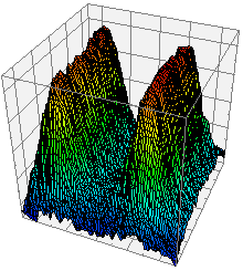
Figure 36. 3D illuminance plot.
To create a plot of the illuminance of a selected area (Figure 36), click
View 3D Plot. The 3D plot will appear in a
new window. The plot can be viewed at any angle by clicking and
dragging. Hold control while dragging to move the plot.
Roll the mouse wheel to zoom in and out. Various plotting options are
available on the right side of the window.
The Blot Report is an exportable table that includes custom names,
number of pixels selected, mean pixel intensities, and standard deviations.
To add a selection to the table, click Add to Report.
You can add as many entries as you would like. The information for the current
selection is shown at the bottom of the drop-down. The table can be viewed and
edited at any time by clicking View Report.
To view the pixel coordinates and intensities for a selection,
click the blue # Pixels label.
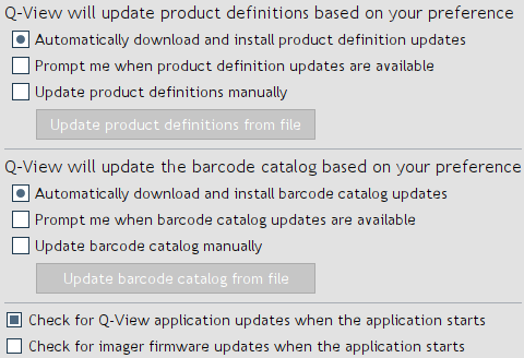
Figure 37. Update options.
Software, product definitions, barcode catalog, and imager firmware updates can be obtained automatically if
set to do so in
Settings > Administration > Q-View Updates (Figure 37). If updates
are not occurring, your network settings may need to be modified in
Settings > Administration > Network Settings.
If your computer does not have Internet access, contact Quansys Biosciences at
sales@quansysbio.com
or 1-888-782-6797 to arrange for regular software
updates to be sent to you.
To apply product catalog updates manually, go to
Settings > Administration > Q-View Updates and select
Update product definitions manually, then click the
Update product definitions from file button. A file selection
window will appear. Navigate to the product definitions file you
received from Quansys Biosciences and select
Open.
To apply barcode catalog updates manually, go to
Settings > Administration > Q-View Updates and select
Update barcode catalog manually, then click the
Update barcode catalog from file button. A file selection
window will appear. Navigate to the barcode catalog file you
received from Quansys Biosciences and select
Open.
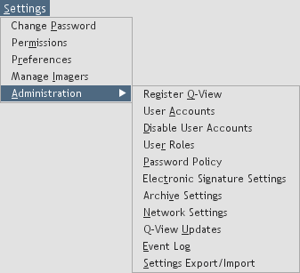
Figure 38. Administrative options.
Use the options under the
Settings menu as follows (Figure 38):
-
Change Password:
Change the password of the currently logged in user.
-
Permissions:
View the permissions of the currently logged in user.
-
Preferences:
Set preferences for auto-set plate overlay, negative well subtraction, reporting,
Q-View Imager Pro temperature regulation, image stacking, notifications and internal illumination.
-
Manage Imagers:
Discover, name, focus, capture dark fields and update firmware for Q-View imagers.
-
Administration:
When logged in as an administrator, you have access to the following settings:
-
Register Q-View:
Enter your company name and assigned license key to
unlock all of the software's features.
-
User Accounts:
Create, delete, or edit user accounts.
-
Disable User Accounts:
User login will no longer be required to use Q-View Software.
-
User Roles:
Manage user roles and permissions.
-
Password Policy:
Manage your organization's password policy.
-
Electronic Signature Settings:
Manage electronic signature settings.
-
Archive Settings:
Enable or disable automatic image archiving and set the retention period.
-
Network Settings:
Specify settings for Internet access for software updates.
If the computer running Q-View Software has multiple network devices,
you may need to manually select the device that has access
to the Internet in order to receive updates.
To select a network device, deselect the Auto-select check
box and choose the network interface and IP address
from which Internet traffic will originate.
If access goes through a proxy, click the
Internet connection requires proxy
check box and enter the IP address or host name and
associated port number. If your proxy requires authentication,
enter the user name and password.
-
Q-View Updates:
Set both software and product definition update preferences.
-
Event Log: View logged application events.
-
Settings Export/Import:
To ease the administrative burden of managing multiple installations of Q-View Software,
settings from one installation of Q-View Software can be exported as a configuration file and imported
into other installations of Q-View Software. This feature is only available when User Accounts are enabled.
The applicable settings are user roles, user accounts and preferences,
password policy, electronic signature settings, archive settings, Q-View update settings, network settings, Q-View imager qualification settings,
and imager & software IQ/OQ settings.

Figure 39. Event log.
A variety of events and setting modifications are recorded in the event log. The event log (Figure 39) can be accessed under Settings > Administration > Event Log.
Events can be filtered by type, user, and date. The log can be exported by clicking the Export button.
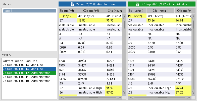
Figure 40. Project history.
Whenever a project is closed or a report is exported, the full report is recorded if any changes exist.
Project history (Figure 40) can be accessed by opening Project > Project History.
By selecting two entries in the history list, you can compare reports to identify differences. Differences are highlighted in yellow.
Reports can exported by clicking the associated Export button.
Q-View Software can be uninstalled through your computer’s settings or by opening the Q-View Software installer and clicking Remove.

Figure 41. Help button.
This manual is available in the software by clicking the help button (Figure 41),
under
Support > Q-View Software Manual, and online at
www.quansysbio.com/manuals.
Tips for many aspects of using multiplex ELISA's are available online at
www.quansysbio.com/tech-tips.
Technical support data such as projects and imager databases can be sent to Quansys Biosciences directly
from Q-View Software by opening
Support > Technical Support Upload and selecting either
Upload Project or
Upload Imager Database. If your computer is not
connected to the Internet, the upload options will prepare the data for manual upload which is accomplished
by moving the produced file(s) to a computer with Internet access and visiting
support.quansysbio.com.
To contact Quansys Biosciences, please:
Call us direct at 1-435-752-0531
or Toll Free within the US 1-888-QUANSYS (888-782-6797)
Email us at
sales@quansysbio.com
for software or other product requests
Email us at
support@quansysbio.com
for technical and troubleshooting issues
Email us at
info@quansysbio.com
for other general inquiries