CC-BY 2015 Lumen Learning

MATH 1314: College Algebra by Lumen Learning is licensed under a Creative Commons Attribution 4.0 International License, except where otherwise noted.
CC-BY 2015 Lumen Learning
MATH 1314: College Algebra by Lumen Learning is licensed under a Creative Commons Attribution 4.0 International License, except where otherwise noted.
By the end of this section, you will be able to:
It is often said that mathematics is the language of science. If this is true, then the language of mathematics is numbers. The earliest use of numbers occurred 100 centuries ago in the Middle East to count, or enumerate items. Farmers, cattlemen, and tradesmen used tokens, stones, or markers to signify a single quantity—a sheaf of grain, a head of livestock, or a fixed length of cloth, for example. Doing so made commerce possible, leading to improved communications and the spread of civilization.
Three to four thousand years ago, Egyptians introduced fractions. They first used them to show reciprocals. Later, they used them to represent the amount when a quantity was divided into equal parts.
But what if there were no cattle to trade or an entire crop of grain was lost in a flood? How could someone indicate the existence of nothing? From earliest times, people had thought of a “base state” while counting and used various symbols to represent this null condition. However, it was not until about the fifth century A.D. in India that zero was added to the number system and used as a numeral in calculations.
Clearly, there was also a need for numbers to represent loss or debt. In India, in the seventh century A.D., negative numbers were used as solutions to mathematical equations and commercial debts. The opposites of the counting numbers expanded the number system even further.
Because of the evolution of the number system, we can now perform complex calculations using these and other categories of real numbers. In this section, we will explore sets of numbers, calculations with different kinds of numbers, and the use of numbers in expressions.
The numbers we use for counting, or enumerating items, are the natural numbers: 1, 2, 3, 4, 5, and so on. We describe them in set notation as {1, 2, 3, …} where the ellipsis (…) indicates that the numbers continue to infinity. The natural numbers are, of course, also called the counting numbers. Any time we enumerate the members of a team, count the coins in a collection, or tally the trees in a grove, we are using the set of natural numbers. The set of whole numbers is the set of natural numbers plus zero: {0, 1, 2, 3,…}.
The set of integers adds the opposites of the natural numbers to the set of whole numbers: {…-3, -2, -1, 0, 1, 2, 3,…}. It is useful to note that the set of integers is made up of three distinct subsets: negative integers, zero, and positive integers. In this sense, the positive integers are just the natural numbers. Another way to think about it is that the natural numbers are a subset of the integers.
The set of rational numbers is written as [latex]\left\{\frac{m}{n}|m\text{ and }{n}\text{ are integers and }{n}\ne{ 0 }\right\}[/latex]. Notice from the definition that rational numbers are fractions (or quotients) containing integers in both the numerator and the denominator, and the denominator is never 0. We can also see that every natural number, whole number, and integer is a rational number with a denominator of 1.
Because they are fractions, any rational number can also be expressed in decimal form. Any rational number can be represented as either:
We use a line drawn over the repeating block of numbers instead of writing the group multiple times.
Write each of the following as a rational number.
Write a fraction with the integer in the numerator and 1 in the denominator.
Write each of the following rational numbers as either a terminating or repeating decimal.
Write each fraction as a decimal by dividing the numerator by the denominator.
Write each of the following rational numbers as either a terminating or repeating decimal.
a. [latex]\frac{68}{17}\\[/latex]
b. [latex]\frac{8}{13}\\[/latex]
c. [latex]-\frac{17}{20}\\[/latex]
At some point in the ancient past, someone discovered that not all numbers are rational numbers. A builder, for instance, may have found that the diagonal of a square with unit sides was not 2 or even [latex]\frac{3}{2}\\[/latex], but was something else. Or a garment maker might have observed that the ratio of the circumference to the diameter of a roll of cloth was a little bit more than 3, but still not a rational number. Such numbers are said to be irrational because they cannot be written as fractions. These numbers make up the set of irrational numbers. Irrational numbers cannot be expressed as a fraction of two integers. It is impossible to describe this set of numbers by a single rule except to say that a number is irrational if it is not rational. So we write this as shown.
Determine whether each of the following numbers is rational or irrational. If it is rational, determine whether it is a terminating or repeating decimal.
So, [latex]\frac{33}{9}\\[/latex] is rational and a repeating decimal.
So, [latex]\frac{17}{34}\\[/latex] is rational and a terminating decimal.
Determine whether each of the following numbers is rational or irrational. If it is rational, determine whether it is a terminating or repeating decimal.
a. [latex]\frac{7}{77}\\[/latex]
b. [latex]\sqrt{81}\\[/latex]
c. [latex]4.27027002700027\dots\\[/latex]
d. [latex]\frac{91}{13}\\[/latex]
e. [latex]\sqrt{39}\\[/latex]
Given any number n, we know that n is either rational or irrational. It cannot be both. The sets of rational and irrational numbers together make up the set of real numbers. As we saw with integers, the real numbers can be divided into three subsets: negative real numbers, zero, and positive real numbers. Each subset includes fractions, decimals, and irrational numbers according to their algebraic sign (+ or –). Zero is considered neither positive nor negative.
The real numbers can be visualized on a horizontal number line with an arbitrary point chosen as 0, with negative numbers to the left of 0 and positive numbers to the right of 0. A fixed unit distance is then used to mark off each integer (or other basic value) on either side of 0. Any real number corresponds to a unique position on the number line.The converse is also true: Each location on the number line corresponds to exactly one real number. This is known as a one-to-one correspondence. We refer to this as the real number line as shown in Figure 1.
Figure 1. The real number line
Classify each number as either positive or negative and as either rational or irrational. Does the number lie to the left or the right of 0 on the number line?
Classify each number as either positive or negative and as either rational or irrational. Does the number lie to the left or the right of 0 on the number line?
a. [latex]\sqrt{73}\\[/latex]
b. [latex]-11.411411411\dots [/latex]
c. [latex]\frac{47}{19}[/latex]
d. [latex]-\frac{\sqrt{5}}{2}[/latex]
e. [latex]6.210735[/latex]
Beginning with the natural numbers, we have expanded each set to form a larger set, meaning that there is a subset relationship between the sets of numbers we have encountered so far. These relationships become more obvious when seen as a diagram.
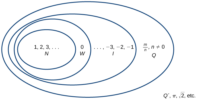
Figure 2. Sets of numbers. N: the set of natural numbers W: the set of whole numbers I: the set of integers Q: the set of rational numbers Q´: the set of irrational numbers
The set of natural numbers includes the numbers used for counting: [latex]\{1,2,3,\dots\}[/latex].
The set of whole numbers is the set of natural numbers plus zero: [latex]\{0,1,2,3,\dots\}[/latex].
The set of integers adds the negative natural numbers to the set of whole numbers: [latex]\{\dots,-3,-2,-1,0,1,2,3,\dots\}[/latex].
The set of rational numbers includes fractions written as [latex]\{\frac{m}{n}|m\text{ and }n\text{ are integers and }n\ne 0\}[/latex].
The set of irrational numbers is the set of numbers that are not rational, are nonrepeating, and are nonterminating: [latex]\{h|h\text{ is not a rational number}\}[/latex].
Classify each number as being a natural number (N), whole number (W), integer (I), rational number (Q), and/or irrational number (Q’).
| N | W | I | Q | Q’ | |
|---|---|---|---|---|---|
| 1. [latex]\sqrt{36}=6[/latex] | X | X | X | X | |
| 2. [latex]\frac{8}{3}=2.\overline{6}[/latex] | X | ||||
| 3. [latex]\sqrt{73}\\[/latex] | X | ||||
| 4. –6 | X | X | |||
| 5. [latex]3.2121121112\dots[/latex] | X |
Classify each number as being a natural number (N), whole number (W), integer (I), rational number (Q), and/or irrational number (Q’).
a. [latex]-\frac{35}{7}[/latex]
b. [latex]0[/latex]
c. [latex]\sqrt{169}[/latex]
d. [latex]\sqrt{24}[/latex]
e. [latex]4.763763763\dots [/latex]
When we multiply a number by itself, we square it or raise it to a power of 2. For example, [latex]{4}^{2}=4\cdot 4=16[/latex]. We can raise any number to any power. In general, the exponential notation [latex]{a}^{n}[/latex] means that the number or variable [latex]a[/latex] is used as a factor [latex]n[/latex] times.
In this notation, [latex]{a}^{n}[/latex] is read as the nth power of [latex]a[/latex], where [latex]a[/latex] is called the base and [latex]n[/latex] is called the exponent. A term in exponential notation may be part of a mathematical expression, which is a combination of numbers and operations. For example, [latex]24+6\cdot \frac{2}{3}-{4}^{2}[/latex] is a mathematical expression.
To evaluate a mathematical expression, we perform the various operations. However, we do not perform them in any random order. We use the order of operations. This is a sequence of rules for evaluating such expressions.
Recall that in mathematics we use parentheses ( ), brackets [ ], and braces { } to group numbers and expressions so that anything appearing within the symbols is treated as a unit. Additionally, fraction bars, radicals, and absolute value bars are treated as grouping symbols. When evaluating a mathematical expression, begin by simplifying expressions within grouping symbols.
The next step is to address any exponents or radicals. Afterward, perform multiplication and division from left to right and finally addition and subtraction from left to right.
Let’s take a look at the expression provided.
There are no grouping symbols, so we move on to exponents or radicals. The number 4 is raised to a power of 2, so simplify [latex]{4}^{2}[/latex] as 16.
Next, perform multiplication or division, left to right.
Lastly, perform addition or subtraction, left to right.
Therefore, [latex]24+6\cdot \frac{2}{3}-{4}^{2}=12[/latex].
For some complicated expressions, several passes through the order of operations will be needed. For instance, there may be a radical expression inside parentheses that must be simplified before the parentheses are evaluated. Following the order of operations ensures that anyone simplifying the same mathematical expression will get the same result.
Operations in mathematical expressions must be evaluated in a systematic order, which can be simplified using the acronym PEMDAS:
P(arentheses)
E(xponents)
M(ultiplication) and D(ivision)
A(ddition) and S(ubtraction)
Use the order of operations to evaluate each of the following expressions.
[latex]\begin{array}{cccc}\left(3\cdot 2\right)^{2} \hfill& =\left(6\right)^{2}-4\left(8\right) \hfill& \text{Simplify parentheses} \\ \hfill& =36-4\left(8\right) \hfill& \text{Simplify exponent} \\ \hfill& =36-32 \hfill& \text{Simplify multiplication} \\ \hfill& =4 \hfill& \text{Simplify subtraction}\end{array}[/latex]
[latex]\begin{array}{cccc}\frac{5^{2}}{7}-\sqrt{11-2} \hfill& =\frac{5^{2}-4}{7}-\sqrt{9} \hfill& \text{Simplify grouping systems (radical)} \\ \hfill& =\frac{5^{2}-4}{7}-3 \hfill& \text{Simplify radical} \\ \hfill& =\frac{25-4}{7}-3 \hfill& \text{Simplify exponent} \\ \hfill& =\frac{21}{7}-3 \hfill& \text{Simplify subtraction in numerator} \\ \hfill& =3-3 \hfill& \text{Simplify division} \\ \hfill& =0 \hfill& \text{Simplify subtraction}\end{array}[/latex]
Note that in the first step, the radical is treated as a grouping symbol, like parentheses. Also, in the third step, the fraction bar is considered a grouping symbol so the numerator is considered to be grouped.
Use the order of operations to evaluate each of the following expressions.
a. [latex]\sqrt{{5}^{2}-{4}^{2}}+7{\left(5 - 4\right)}^{2}[/latex]
b. [latex]1+\frac{7\cdot 5 - 8\cdot 4}{9 - 6}[/latex]
c. [latex]|1.8 - 4.3|+0.4\sqrt{15+10}[/latex]
d. [latex]\frac{1}{2}\left[5\cdot {3}^{2}-{7}^{2}\right]+\frac{1}{3}\cdot {9}^{2}[/latex]
e. [latex][{\left(3 - 8\right)}^{2}-4]-\left(3 - 8\right)[/latex]
For some activities we perform, the order of certain operations does not matter, but the order of other operations does. For example, it does not make a difference if we put on the right shoe before the left or vice-versa. However, it does matter whether we put on shoes or socks first. The same thing is true for operations in mathematics.
The commutative property of addition states that numbers may be added in any order without affecting the sum.
We can better see this relationship when using real numbers.
Similarly, the commutative property of multiplication states that numbers may be multiplied in any order without affecting the product.
Again, consider an example with real numbers.
It is important to note that neither subtraction nor division is commutative. For example, [latex]17 - 5[/latex] is not the same as [latex]5 - 17[/latex]. Similarly, [latex]20\div 5\ne 5\div 20[/latex].
The associative property of multiplication tells us that it does not matter how we group numbers when multiplying. We can move the grouping symbols to make the calculation easier, and the product remains the same.
Consider this example.
The associative property of addition tells us that numbers may be grouped differently without affecting the sum.
This property can be especially helpful when dealing with negative integers. Consider this example.
Are subtraction and division associative? Review these examples.
As we can see, neither subtraction nor division is associative.
The distributive property states that the product of a factor times a sum is the sum of the factor times each term in the sum.
This property combines both addition and multiplication (and is the only property to do so). Let us consider an example.

Note that 4 is outside the grouping symbols, so we distribute the 4 by multiplying it by 12, multiplying it by –7, and adding the products.
To be more precise when describing this property, we say that multiplication distributes over addition. The reverse is not true, as we can see in this example.
Multiplication does not distribute over subtraction, and division distributes over neither addition nor subtraction.
A special case of the distributive property occurs when a sum of terms is subtracted.
For example, consider the difference [latex]12-\left(5+3\right)[/latex]. We can rewrite the difference of the two terms 12 and [latex]\left(5+3\right)[/latex] by turning the subtraction expression into addition of the opposite. So instead of subtracting [latex]\left(5+3\right)[/latex], we add the opposite.
Now, distribute [latex]-1[/latex] and simplify the result.
This seems like a lot of trouble for a simple sum, but it illustrates a powerful result that will be useful once we introduce algebraic terms. To subtract a sum of terms, change the sign of each term and add the results. With this in mind, we can rewrite the last example.
The identity property of addition states that there is a unique number, called the additive identity (0) that, when added to a number, results in the original number.
The identity property of multiplication states that there is a unique number, called the multiplicative identity (1) that, when multiplied by a number, results in the original number.
For example, we have [latex]\left(-6\right)+0=-6[/latex] and [latex]23\cdot 1=23[/latex]. There are no exceptions for these properties; they work for every real number, including 0 and 1.
The inverse property of addition states that, for every real number a, there is a unique number, called the additive inverse (or opposite), denoted−a, that, when added to the original number, results in the additive identity, 0.
For example, if [latex]a=-8[/latex], the additive inverse is 8, since [latex]\left(-8\right)+8=0[/latex].
The inverse property of multiplication holds for all real numbers except 0 because the reciprocal of 0 is not defined. The property states that, for every real number a, there is a unique number, called the multiplicative inverse (or reciprocal), denoted [latex]\frac{1}{a}[/latex], that, when multiplied by the original number, results in the multiplicative identity, 1.
For example, if [latex]a=-\frac{2}{3}[/latex], the reciprocal, denoted [latex]\frac{1}{a}[/latex], is [latex]-\frac{3}{2}[/latex] because
The following properties hold for real numbers a, b, and c.
| Addition | Multiplication | |
|---|---|---|
| Commutative Property | [latex]a+b=b+a[/latex] | [latex]a\cdot b=b\cdot a[/latex] |
| Associative Property | [latex]a+\left(b+c\right)=\left(a+b\right)+c[/latex] | [latex]a\left(bc\right)=\left(ab\right)c[/latex] |
| Distributive Property | [latex]a\cdot \left(b+c\right)=a\cdot b+a\cdot c[/latex] | |
| Identity Property | There exists a unique real number called the additive identity, 0, such that, for any real number a [latex]a+0=a[/latex] | There exists a unique real number called the multiplicative identity, 1, such that, for any real number a [latex]a\cdot 1=a[/latex] |
| Inverse Property | Every real number a has an additive inverse, or opposite, denoted –a, such that [latex]a+\left(-a\right)=0[/latex] | Every nonzero real number a has a multiplicative inverse, or reciprocal, denoted [latex]\frac{1}{a}[/latex], such that [latex]a\cdot \left(\frac{1}{a}\right)=1[/latex] |
Use the properties of real numbers to rewrite and simplify each expression. State which properties apply.
Use the properties of real numbers to rewrite and simplify each expression. State which properties apply.
a. [latex]\left(-\frac{23}{5}\right)\cdot \left[11\cdot \left(-\frac{5}{23}\right)\right][/latex]
b. [latex]5\cdot \left(6.2+0.4\right)[/latex]
c. [latex]18-\left(7 - 15\right)[/latex]
d. [latex]\frac{17}{18}+\cdot \left[\frac{4}{9}+\left(-\frac{17}{18}\right)\right][/latex]
e. [latex]6\cdot \left(-3\right)+6\cdot 3[/latex]
So far, the mathematical expressions we have seen have involved real numbers only. In mathematics, we may see expressions such as [latex]x+5,\frac{4}{3}\pi {r}^{3}[/latex], or [latex]\sqrt{2{m}^{3}{n}^{2}}[/latex]. In the expression [latex]x+5[/latex], 5 is called a constant because it does not vary and x is called a variable because it does. (In naming the variable, ignore any exponents or radicals containing the variable.) An algebraic expression is a collection of constants and variables joined together by the algebraic operations of addition, subtraction, multiplication, and division.
We have already seen some real number examples of exponential notation, a shorthand method of writing products of the same factor. When variables are used, the constants and variables are treated the same way.
In each case, the exponent tells us how many factors of the base to use, whether the base consists of constants or variables.
Any variable in an algebraic expression may take on or be assigned different values. When that happens, the value of the algebraic expression changes. To evaluate an algebraic expression means to determine the value of the expression for a given value of each variable in the expression. Replace each variable in the expression with the given value, then simplify the resulting expression using the order of operations. If the algebraic expression contains more than one variable, replace each variable with its assigned value and simplify the expression as before.
List the constants and variables for each algebraic expression.
| Constants | Variables | |
|---|---|---|
| 1. x + 5 | 5 | x |
| 2. [latex]\frac{4}{3}\pi {r}^{3}[/latex] | [latex]\frac{4}{3},\pi [/latex] | [latex]r[/latex] |
| 3. [latex]\sqrt{2{m}^{3}{n}^{2}}[/latex] | 2 | [latex]m,n[/latex] |
List the constants and variables for each algebraic expression.
Evaluate the expression [latex]2x - 7[/latex] for each value for x.
Evaluate the expression [latex]11 - 3y[/latex] for each value for y.
a. [latex]y=2[/latex]
b. [latex]y=0[/latex]
c. [latex]y=\frac{2}{3}[/latex]
d. [latex]y=-5[/latex]
Evaluate each expression for the given values.
Evaluate each expression for the given values.
a. [latex]\frac{y+3}{y - 3}[/latex] for [latex]y=5[/latex]
b. [latex]7 - 2t[/latex] for [latex]t=-2[/latex]
c. [latex]\frac{1}{3}\pi {r}^{2}[/latex] for [latex]r=11[/latex]
d. [latex]{\left({p}^{2}q\right)}^{3}[/latex] for [latex]p=-2,q=3[/latex]
e. [latex]4\left(m-n\right)-5\left(n-m\right)[/latex] for [latex]m=\frac{2}{3},n=\frac{1}{3}[/latex]
An equation is a mathematical statement indicating that two expressions are equal. The expressions can be numerical or algebraic. The equation is not inherently true or false, but only a proposition. The values that make the equation true, the solutions, are found using the properties of real numbers and other results. For example, the equation [latex]2x+1=7[/latex] has the unique solution [latex]x=3[/latex] because when we substitute 3 for [latex]x[/latex] in the equation, we obtain the true statement [latex]2\left(3\right)+1=7[/latex].
A formula is an equation expressing a relationship between constant and variable quantities. Very often, the equation is a means of finding the value of one quantity (often a single variable) in terms of another or other quantities. One of the most common examples is the formula for finding the area [latex]A[/latex] of a circle in terms of the radius [latex]r[/latex] of the circle: [latex]A=\pi {r}^{2}[/latex]. For any value of [latex]r[/latex], the area [latex]A[/latex] can be found by evaluating the expression [latex]\pi {r}^{2}[/latex].
A right circular cylinder with radius [latex]r[/latex] and height [latex]h[/latex] has the surface area [latex]S[/latex] (in square units) given by the formula [latex]S=2\pi r\left(r+h\right)[/latex]. Find the surface area of a cylinder with radius 6 in. and height 9 in. Leave the answer in terms of [latex]\pi[/latex].
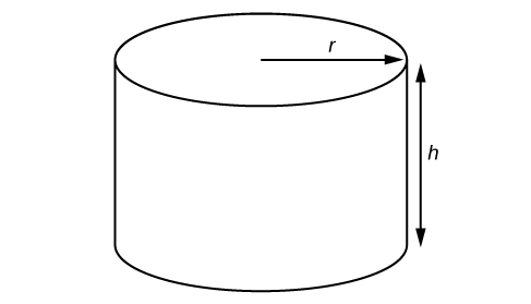
Figure 3. Right circular cylinder
Evaluate the expression [latex]2\pi r\left(r+h\right)[/latex] for [latex]r=6[/latex] and [latex]h=9[/latex].
The surface area is [latex]180\pi [/latex] square inches.
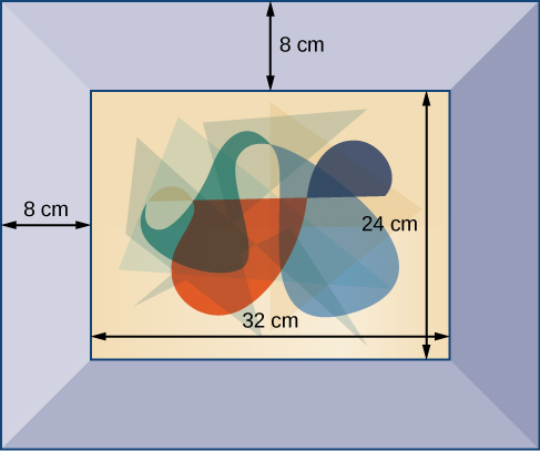
Figure 4
A photograph with length L and width W is placed in a matte of width 8 centimeters (cm). The area of the matte (in square centimeters, or cm2) is found to be [latex]A=\left(L+16\right)\left(W+16\right)-L\cdot W[/latex]. Find the area of a matte for a photograph with length 32 cm and width 24 cm.
Sometimes we can simplify an algebraic expression to make it easier to evaluate or to use in some other way. To do so, we use the properties of real numbers. We can use the same properties in formulas because they contain algebraic expressions.
Simplify each algebraic expression.
Simplify each algebraic expression.
A rectangle with length [latex]L[/latex] and width [latex]W[/latex] has a perimeter [latex]P[/latex] given by [latex]P=L+W+L+W[/latex]. Simplify this expression.
If the amount [latex]P[/latex] is deposited into an account paying simple interest [latex]r[/latex] for time [latex]t[/latex], the total value of the deposit [latex]A[/latex] is given by [latex]A=P+Prt[/latex]. Simplify the expression. (This formula will be explored in more detail later in the course.)
algebraic expression constants and variables combined using addition, subtraction, multiplication, and division
associative property of addition the sum of three numbers may be grouped differently without affecting the result; in symbols, [latex]a+\left(b+c\right)=\left(a+b\right)+c[/latex]
associative property of multiplication the product of three numbers may be grouped differently without affecting the result; in symbols, [latex]a\cdot \left(b\cdot c\right)=\left(a\cdot b\right)\cdot c[/latex]
base in exponential notation, the expression that is being multiplied
commutative property of addition two numbers may be added in either order without affecting the result; in symbols, [latex]a+b=b+a[/latex]
commutative property of multiplication two numbers may be multiplied in any order without affecting the result; in symbols, [latex]a\cdot b=b\cdot a[/latex]
constant a quantity that does not change value
distributive property the product of a factor times a sum is the sum of the factor times each term in the sum; in symbols, [latex]a\cdot \left(b+c\right)=a\cdot b+a\cdot c[/latex]
equation a mathematical statement indicating that two expressions are equal
exponent in exponential notation, the raised number or variable that indicates how many times the base is being multiplied
exponential notation a shorthand method of writing products of the same factor
formula an equation expressing a relationship between constant and variable quantities
identity property of addition there is a unique number, called the additive identity, 0, which, when added to a number, results in the original number; in symbols, [latex]a+0=a[/latex]
identity property of multiplication there is a unique number, called the multiplicative identity, 1, which, when multiplied by a number, results in the original number; in symbols, [latex]a\cdot 1=a[/latex]
integers the set consisting of the natural numbers, their opposites, and 0: [latex]\{\dots ,-3,-2,-1,0,1,2,3,\dots \}[/latex]
inverse property of addition for every real number [latex]a[/latex], there is a unique number, called the additive inverse (or opposite), denoted [latex]-a[/latex], which, when added to the original number, results in the additive identity, 0; in symbols, [latex]a+\left(-a\right)=0[/latex]
inverse property of multiplication for every non-zero real number [latex]a[/latex], there is a unique number, called the multiplicative inverse (or reciprocal), denoted [latex]\frac{1}{a}[/latex], which, when multiplied by the original number, results in the multiplicative identity, 1; in symbols, [latex]a\cdot \frac{1}{a}=1[/latex]
irrational numbers the set of all numbers that are not rational; they cannot be written as either a terminating or repeating decimal; they cannot be expressed as a fraction of two integers
natural numbers the set of counting numbers: [latex]\{1,2,3,\dots \}[/latex]
order of operations a set of rules governing how mathematical expressions are to be evaluated, assigning priorities to operations
rational numbers the set of all numbers of the form [latex]\frac{m}{n}[/latex], where [latex]m[/latex] and [latex]n[/latex] are integers and [latex]n\ne 0[/latex]. Any rational number may be written as a fraction or a terminating or repeating decimal.
real number line a horizontal line used to represent the real numbers. An arbitrary fixed point is chosen to represent 0; positive numbers lie to the right of 0 and negative numbers to the left.
real numbers the sets of rational numbers and irrational numbers taken together
variable a quantity that may change value
whole numbers the set consisting of 0 plus the natural numbers: [latex]\{0,1,2,3,\dots \}[/latex]
1. Is [latex]\sqrt{2}[/latex] an example of a rational terminating, rational repeating, or irrational number? Tell why it fits that category.
2. What is the order of operations? What acronym is used to describe the order of operations, and what does it stand for?
3. What do the Associative Properties allow us to do when following the order of operations? Explain your answer.
For the following exercises, simplify the given expression.
4. [latex]10+2\times \left(5 - 3\right)[/latex]
5. [latex]6\div 2-\left(81\div {3}^{2}\right)[/latex]
6. [latex]18+{\left(6 - 8\right)}^{3}[/latex]
7. [latex]-2\times {\left[16\div {\left(8 - 4\right)}^{2}\right]}^{2}[/latex]
8. [latex]4 - 6+2\times 7[/latex]
9. [latex]3\left(5 - 8\right)[/latex]
10. [latex]4+6 - 10\div 2[/latex]
11. [latex]12\div \left(36\div 9\right)+6[/latex]
12. [latex]{\left(4+5\right)}^{2}\div 3[/latex]
13. [latex]3 - 12\times 2+19[/latex]
14. [latex]2+8\times 7\div 4[/latex]
15. [latex]5+\left(6+4\right)-11[/latex]
16. [latex]9 - 18\div {3}^{2}[/latex]
17. [latex]14\times 3\div 7 - 6[/latex]
18. [latex]9-\left(3+11\right)\times 2[/latex]
19. [latex]6+2\times 2 - 1[/latex]
20. [latex]64\div \left(8+4\times 2\right)[/latex]
21. [latex]9+4\left({2}^{2}\right)[/latex]
22. [latex]{\left(12\div 3\times 3\right)}^{2}[/latex]
23. [latex]25\div {5}^{2}-7[/latex]
24. [latex]\left(15 - 7\right)\times \left(3 - 7\right)[/latex]
25. [latex]2\times 4 - 9\left(-1\right)[/latex]
26. [latex]{4}^{2}-25\times \frac{1}{5}[/latex]
27. [latex]12\left(3 - 1\right)\div 6[/latex]
For the following exercises, solve for the variable.
28. [latex]8\left(x+3\right)=64[/latex]
29. [latex]4y+8=2y[/latex]
30. [latex]\left(11a+3\right)-18a=-4[/latex]
31. [latex]4z - 2z\left(1+4\right)=36[/latex]
32. [latex]4y{\left(7 - 2\right)}^{2}=-200[/latex]
33. [latex]-{\left(2x\right)}^{2}+1=-3[/latex]
34. [latex]8\left(2+4\right)-15b=b[/latex]
35. [latex]2\left(11c - 4\right)=36[/latex]
36. [latex]4\left(3 - 1\right)x=4[/latex]
37. [latex]\frac{1}{4}\left(8w-{4}^{2}\right)=0[/latex]
For the following exercises, simplify the expression.
38. [latex]4x+x\left(13 - 7\right)[/latex]
39. [latex]2y-{\left(4\right)}^{2}y - 11[/latex]
40. [latex]\frac{a}{{2}^{3}}\left(64\right)-12a\div 6[/latex]
41. [latex]8b - 4b\left(3\right)+1[/latex]
42. [latex]5l\div 3l\times \left(9 - 6\right)[/latex]
43. [latex]7z - 3+z\times {6}^{2}[/latex]
44. [latex]4\times 3+18x\div 9 - 12[/latex]
45. [latex]9\left(y+8\right)-27[/latex]
46. [latex]\left(\frac{9}{6}t - 4\right)2[/latex]
47. [latex]6+12b - 3\times 6b[/latex]
48. [latex]18y - 2\left(1+7y\right)[/latex]
49. [latex]{\left(\frac{4}{9}\right)}^{2}\times 27x[/latex]
50. [latex]8\left(3-m\right)+1\left(-8\right)[/latex]
51. [latex]9x+4x\left(2+3\right)-4\left(2x+3x\right)[/latex]
52. [latex]{5}^{2}-4\left(3x\right)[/latex]
For the following exercises, consider this scenario: Fred earns $40 mowing lawns. He spends $10 on mp3s, puts half of what is left in a savings account, and gets another $5 for washing his neighbor’s car.
53. Write the expression that represents the number of dollars Fred keeps (and does not put in his savings account). Remember the order of operations.
54. How much money does Fred keep?
For the following exercises, solve the given problem.
55. According to the U.S. Mint, the diameter of a quarter is 0.955 inches. The circumference of the quarter would be the diameter multiplied by [latex]\pi [/latex]. Is the circumference of a quarter a whole number, a rational number, or an irrational number?
56. Jessica and her roommate, Adriana, have decided to share a change jar for joint expenses. Jessica put her loose change in the jar first, and then Adriana put her change in the jar. We know that it does not matter in which order the change was added to the jar. What property of addition describes this fact?
For the following exercises, consider this scenario: There is a mound of [latex]g[/latex] pounds of gravel in a quarry. Throughout the day, 400 pounds of gravel is added to the mound. Two orders of 600 pounds are sold and the gravel is removed from the mound. At the end of the day, the mound has 1,200 pounds of gravel.
57. Write the equation that describes the situation.
58. Solve for g.
For the following exercise, solve the given problem.
59. Ramon runs the marketing department at his company. His department gets a budget every year, and every year, he must spend the entire budget without going over. If he spends less than the budget, then his department gets a smaller budget the following year. At the beginning of this year, Ramon got $2.5 million for the annual marketing budget. He must spend the budget such that [latex]2,500,000-x=0[/latex]. What property of addition tells us what the value of x must be?
For the following exercises, use a graphing calculator to solve for x. Round the answers to the nearest hundredth.
60. [latex]0.5{\left(12.3\right)}^{2}-48x=\frac{3}{5}[/latex]
61. [latex]{\left(0.25 - 0.75\right)}^{2}x - 7.2=9.9[/latex]
62. If a whole number is not a natural number, what must the number be?
63. Determine whether the statement is true or false: The multiplicative inverse of a rational number is also rational.
64. Determine whether the statement is true or false: The product of a rational and irrational number is always irrational.
65. Determine whether the simplified expression is rational or irrational: [latex]\sqrt{-18 - 4\left(5\right)\left(-1\right)}[/latex].
66. Determine whether the simplified expression is rational or irrational: [latex]\sqrt{-16+4\left(5\right)+5}[/latex].
67. The division of two whole numbers will always result in what type of number?
68. What property of real numbers would simplify the following expression: [latex]4+7\left(x - 1\right)?[/latex]
1. a. [latex]\frac{11}{1}[/latex]
b. [latex]\frac{3}{1}[/latex]
c. [latex]-\frac{4}{1}[/latex]
2. a. 4 (or 4.0), terminating
b. [latex]0.\overline{615384}[/latex], repeating
c. –0.85, terminating
3. a. rational and repeating
b. rational and terminating
c. irrational
d. rational and repeating
e. irrational
4. a. positive, irrational; right
b. negative, rational; left
c. positive, rational; right
d. negative, irrational; left
e. positive, rational; right
5.
| N | W | I | Q | Q’ | |
|---|---|---|---|---|---|
| a. [latex]-\frac{35}{7}[/latex] | X | X | |||
| b. 0 | X | X | X | ||
| c. [latex]\sqrt{169}[/latex] | X | X | X | X | |
| d. [latex]\sqrt{24}[/latex] | X | ||||
| e. [latex]4.763763763\dots[/latex] | X |
6. a. 10
b. 2
c. 4.5
d. 25
e. 26
7. a. commutative property of multiplication, associative property of multiplication, inverse property of multiplication, identity property of multiplication;
b. 33, distributive property;
c. 26, distributive property;
d. [latex]\frac{4}{9}[/latex], commutative property of addition, associative property of addition, inverse property of addition, identity property of addition;
e. 0, distributive property, inverse property of addition, identity property of addition
8.
| Constants | Variables | |
|---|---|---|
| a. [latex]2\pi r\left(r+h\right)[/latex] | [latex]2,\pi [/latex] | [latex]r,h[/latex] |
| b. 2(L + W) | 2 | L, W |
| c. [latex]4{y}^{3}+y[/latex] | 4 | [latex]y[/latex] |
9. a. 5
b. 11
c. 9
d. 26
10. a. 4
b. 11
c. [latex]\frac{121}{3}\pi [/latex]
d. 1728
e. 3
11. 1,152 cm2
12. a. [latex]-2y - 2z\text{ or }-2\left(y+z\right)[/latex]
b. [latex]\frac{2}{t}-1[/latex]
c. [latex]3pq - 4p+q[/latex]
d. [latex]7r - 2s+6[/latex]
13. [latex]A=P\left(1+rt\right)[/latex]
1. irrational number. The square root of two does not terminate, and it does not repeat a pattern. It cannot be written as a quotient of two integers, so it is irrational.
3. The Associative Properties state that the sum or product of multiple numbers can be grouped differently without affecting the result. This is because the same operation is performed (either addition or subtraction), so the terms can be re-ordered.
5. [latex]-6[/latex]
7. [latex]-2[/latex]
9. [latex]-9[/latex]
11. 9
13. 4
15. 4
17. 0
19. 9
21. 25
23. [latex]-6[/latex]
25. 17
27. 4
29. [latex]-4[/latex]
31. [latex]-6[/latex]
33. [latex]\pm 1[/latex]
35. 2
37. 2
39. [latex]-14y - 11[/latex]
41. [latex]-4b+1[/latex]
43. [latex]43z - 3[/latex]
45. [latex]9y+45[/latex]
47. [latex]-6b+6[/latex]
49. [latex]\frac{16x}{3}\\[/latex]
51. [latex]9x[/latex]
53. [latex]\frac{1}{2}\left(40 - 10\right)+5[/latex]
55. irrational number
57. [latex]g+400 - 2\left(600\right)=1200[/latex]
59. inverse property of addition
61. 68.4
63. true
65. irrational
67. rational
By the end of this section, you will be able to:
Caroline is a full-time college student planning a spring break vacation. To earn enough money for the trip, she has taken a part-time job at the local bank that pays $15.00/hr, and she opened a savings account with an initial deposit of $400 on January 15. She arranged for direct deposit of her payroll checks. If spring break begins March 20 and the trip will cost approximately $2,500, how many hours will she have to work to earn enough to pay for her vacation? If she can only work 4 hours per day, how many days per week will she have to work? How many weeks will it take? In this section, we will investigate problems like this and others, which generate graphs like the line in Figure 1.
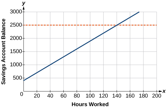
Figure 1
A linear equation is an equation of a straight line, written in one variable. The only power of the variable is 1. Linear equations in one variable may take the form [latex]ax+b=0[/latex] and are solved using basic algebraic operations.
We begin by classifying linear equations in one variable as one of three types: identity, conditional, or inconsistent. An identity equation is true for all values of the variable. Here is an example of an identity equation.
The solution set consists of all values that make the equation true. For this equation, the solution set is all real numbers because any real number substituted for [latex]x[/latex] will make the equation true.
A conditional equation is true for only some values of the variable. For example, if we are to solve the equation [latex]5x+2=3x - 6[/latex], we have the following:
The solution set consists of one number: [latex]\{-4\}[/latex]. It is the only solution and, therefore, we have solved a conditional equation.
An inconsistent equation results in a false statement. For example, if we are to solve [latex]5x - 15=5\left(x - 4\right)[/latex], we have the following:
Indeed, [latex]-15\ne -20[/latex]. There is no solution because this is an inconsistent equation.
Solving linear equations in one variable involves the fundamental properties of equality and basic algebraic operations. A brief review of those operations follows.
A linear equation in one variable can be written in the form
where a and b are real numbers, [latex]a\ne 0[/latex].
The following steps are used to manipulate an equation and isolate the unknown variable, so that the last line reads x=_________, if x is the unknown. There is no set order, as the steps used depend on what is given:
Solve the following equation: [latex]2x+7=19[/latex].
This equation can be written in the form [latex]ax+b=0[/latex] by subtracting [latex]19[/latex] from both sides. However, we may proceed to solve the equation in its original form by performing algebraic operations.
The solution is [latex]x=6[/latex].
Solve the following equation: [latex]4\left(x - 3\right)+12=15 - 5\left(x+6\right)[/latex].
Apply standard algebraic properties.
This problem requires the distributive property to be applied twice, and then the properties of algebra are used to reach the final line, [latex]x=-\frac{5}{3}[/latex].
In this section, we look at rational equations that, after some manipulation, result in a linear equation. If an equation contains at least one rational expression, it is a considered a rational equation.
Recall that a rational number is the ratio of two numbers, such as [latex]\frac{2}{3}[/latex] or [latex]\frac{7}{2}[/latex]. A rational expression is the ratio, or quotient, of two polynomials. Here are three examples.
Rational equations have a variable in the denominator in at least one of the terms.
Our goal is to perform algebraic operations so that the variables appear in the numerator. In fact, we will eliminate all denominators by multiplying both sides of the equation by the least common denominator (LCD).
Finding the LCD is identifying an expression that contains the highest power of all of the factors in all of the denominators. We do this because when the equation is multiplied by the LCD, the common factors in the LCD and in each denominator will equal one and will cancel out.
Solve the rational equation: [latex]\frac{7}{2x}-\frac{5}{3x}=\frac{22}{3}\\[/latex].
We have three denominators; [latex]2x,3x[/latex], and 3. The LCD must contain [latex]2x,3x[/latex], and 3. An LCD of [latex]6x[/latex] contains all three denominators. In other words, each denominator can be divided evenly into the LCD. Next, multiply both sides of the equation by the LCD [latex]6x[/latex].
A common mistake made when solving rational equations involves finding the LCD when one of the denominators is a binomial—two terms added or subtracted—such as [latex]\left(x+1\right)[/latex]. Always consider a binomial as an individual factor—the terms cannot be separated. For example, suppose a problem has three terms and the denominators are [latex]x[/latex], [latex]x - 1[/latex], and [latex]3x - 3[/latex]. First, factor all denominators. We then have [latex]x[/latex], [latex]\left(x - 1\right)[/latex], and [latex]3\left(x - 1\right)[/latex] as the denominators. (Note the parentheses placed around the second denominator.) Only the last two denominators have a common factor of [latex]\left(x - 1\right)[/latex]. The [latex]x[/latex] in the first denominator is separate from the [latex]x[/latex] in the [latex]\left(x - 1\right)[/latex] denominators. An effective way to remember this is to write factored and binomial denominators in parentheses, and consider each parentheses as a separate unit or a separate factor. The LCD in this instance is found by multiplying together the [latex]x[/latex], one factor of [latex]\left(x - 1\right)[/latex], and the 3. Thus, the LCD is the following:
So, both sides of the equation would be multiplied by [latex]3x\left(x - 1\right)[/latex]. Leave the LCD in factored form, as this makes it easier to see how each denominator in the problem cancels out.
Another example is a problem with two denominators, such as [latex]x[/latex] and [latex]{x}^{2}+2x[/latex]. Once the second denominator is factored as [latex]{x}^{2}+2x=x\left(x+2\right)[/latex], there is a common factor of x in both denominators and the LCD is [latex]x\left(x+2\right)[/latex].
Sometimes we have a rational equation in the form of a proportion; that is, when one fraction equals another fraction and there are no other terms in the equation.
We can use another method of solving the equation without finding the LCD: cross-multiplication. We multiply terms by crossing over the equal sign.

Multiply [latex]a\left(d\right)[/latex] and [latex]b\left(c\right)[/latex], which results in [latex]ad=bc[/latex].
Any solution that makes a denominator in the original expression equal zero must be excluded from the possibilities.
A rational equation contains at least one rational expression where the variable appears in at least one of the denominators.
Solve the following rational equation:
We have three denominators: [latex]x[/latex], [latex]2[/latex], and [latex]2x[/latex]. No factoring is required. The product of the first two denominators is equal to the third denominator, so, the LCD is [latex]2x[/latex]. Only one value is excluded from a solution set, [latex]x=0[/latex]. Next, multiply the whole equation (both sides of the equal sign) by [latex]2x[/latex].
The proposed solution is [latex]x=-1[/latex], which is not an excluded value, so the solution set contains one number, [latex]x=-1[/latex], or [latex]\{-1\}[/latex] written in set notation.
Solve the rational equation: [latex]\frac{2}{3x}=\frac{1}{4}-\frac{1}{6x}[/latex].
Solve the following rational equation: [latex]\frac{1}{x}=\frac{1}{10}-\frac{3}{4x}[/latex].
First find the common denominator. The three denominators in factored form are [latex]x,10=2\cdot 5[/latex], and [latex]4x=2\cdot 2\cdot x[/latex]. The smallest expression that is divisible by each one of the denominators is [latex]20x[/latex]. Only [latex]x=0[/latex] is an excluded value. Multiply the whole equation by [latex]20x[/latex].
The solution is [latex]x=\frac{35}{2}[/latex].
Solve the rational equation: [latex]-\frac{5}{2x}+\frac{3}{4x}=-\frac{7}{4}[/latex].
Solve the following rational equations and state the excluded values:
The solution is [latex]x=15[/latex]. The excluded values are [latex]x=6[/latex] and [latex]x=0[/latex].
The solution is [latex]x=\frac{13}{3}[/latex]. The excluded value is [latex]x=3[/latex].
The solution is [latex]x=4[/latex]. The excluded value is [latex]x=2[/latex].
Solve the rational equation after factoring the denominators: [latex]\frac{2}{x+1}-\frac{1}{x - 1}=\frac{2x}{{x}^{2}-1}[/latex]. State the excluded values.
We must factor the denominator [latex]{x}^{2}-1[/latex]. We recognize this as the difference of squares, and factor it as [latex]\left(x - 1\right)\left(x+1\right)[/latex]. Thus, the LCD that contains each denominator is [latex]\left(x - 1\right)\left(x+1\right)[/latex]. Multiply the whole equation by the LCD, cancel out the denominators, and solve the remaining equation.
The solution is [latex]x=-3[/latex]. The excluded values are [latex]x=1[/latex] and [latex]x=-1[/latex].
Solve the rational equation: [latex]\frac{2}{x - 2}+\frac{1}{x+1}=\frac{1}{{x}^{2}-x - 2}[/latex].
Perhaps the most familiar form of a linear equation is the slope-intercept form, written as [latex]y=mx+b[/latex], where [latex]m=\text{slope}[/latex] and [latex]b=y\text{-intercept}[/latex]. Let us begin with the slope.
The slope of a line refers to the ratio of the vertical change in y over the horizontal change in x between any two points on a line. It indicates the direction in which a line slants as well as its steepness. Slope is sometimes described as rise over run.
If the slope is positive, the line slants to the right. If the slope is negative, the line slants to the left. As the slope increases, the line becomes steeper. Some examples are shown in Figure 2. The lines indicate the following slopes: [latex]m=-3[/latex], [latex]m=2[/latex], and [latex]m=\frac{1}{3}[/latex].
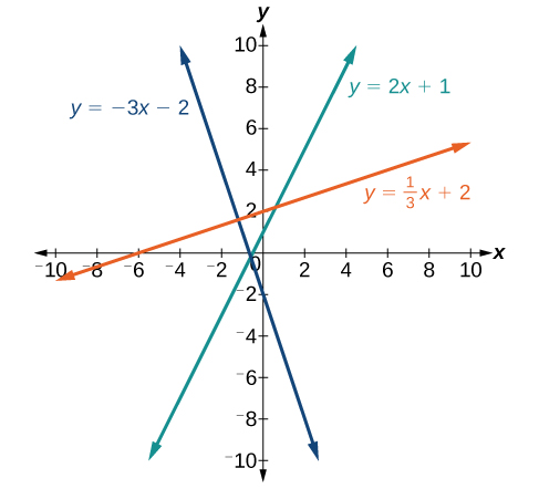
Figure 2
The slope of a line, m, represents the change in y over the change in x. Given two points, [latex]\left({x}_{1},{y}_{1}\right)[/latex] and [latex]\left({x}_{2},{y}_{2}\right)[/latex], the following formula determines the slope of a line containing these points:
Find the slope of a line that passes through the points [latex]\left(2,-1\right)[/latex] and [latex]\left(-5,3\right)[/latex].
We substitute the y-values and the x-values into the formula.
The slope is [latex]-\frac{4}{7}[/latex].
It does not matter which point is called [latex]\left({x}_{1},{y}_{1}\right)[/latex] or [latex]\left({x}_{2},{y}_{2}\right)[/latex]. As long as we are consistent with the order of the y terms and the order of the x terms in the numerator and denominator, the calculation will yield the same result.
Find the slope of the line that passes through the points [latex]\left(-2,6\right)[/latex] and [latex]\left(1,4\right)[/latex].
Identify the slope and y-intercept, given the equation [latex]y=-\frac{3}{4}x - 4[/latex].
As the line is in [latex]y=mx+b[/latex] form, the given line has a slope of [latex]m=-\frac{3}{4}[/latex]. The y-intercept is [latex]b=-4[/latex].
The y-intercept is the point at which the line crosses the y-axis. On the y-axis, [latex]x=0[/latex]. We can always identify the y-intercept when the line is in slope-intercept form, as it will always equal b. Or, just substitute [latex]x=0[/latex] and solve for y.
Given the slope and one point on a line, we can find the equation of the line using the point-slope formula.
This is an important formula, as it will be used in other areas of college algebra and often in calculus to find the equation of a tangent line. We need only one point and the slope of the line to use the formula. After substituting the slope and the coordinates of one point into the formula, we simplify it and write it in slope-intercept form.
Given one point and the slope, the point-slope formula will lead to the equation of a line:
Write the equation of the line with slope [latex]m=-3[/latex] and passing through the point [latex]\left(4,8\right)[/latex]. Write the final equation in slope-intercept form.
Using the point-slope formula, substitute [latex]-3[/latex] for m and the point [latex]\left(4,8\right)[/latex] for [latex]\left({x}_{1},{y}_{1}\right)[/latex].
Note that any point on the line can be used to find the equation. If done correctly, the same final equation will be obtained.
Given [latex]m=4[/latex], find the equation of the line in slope-intercept form passing through the point [latex]\left(2,5\right)[/latex].
Find the equation of the line passing through the points [latex]\left(3,4\right)[/latex] and [latex]\left(0,-3\right)[/latex]. Write the final equation in slope-intercept form.
First, we calculate the slope using the slope formula and two points.
Next, we use the point-slope formula with the slope of [latex]\frac{7}{3}[/latex], and either point. Let’s pick the point [latex]\left(3,4\right)[/latex] for [latex]\left({x}_{1},{y}_{1}\right)[/latex].
In slope-intercept form, the equation is written as [latex]y=\frac{7}{3}x - 3[/latex].
To prove that either point can be used, let us use the second point [latex]\left(0,-3\right)[/latex] and see if we get the same equation.
We see that the same line will be obtained using either point. This makes sense because we used both points to calculate the slope.
Another way that we can represent the equation of a line is in standard form. Standard form is given as
where [latex]A[/latex], [latex]B[/latex], and [latex]C[/latex] are integers. The x- and y-terms are on one side of the equal sign and the constant term is on the other side.
Find the equation of the line with [latex]m=-6[/latex] and passing through the point [latex]\left(\frac{1}{4},-2\right)[/latex]. Write the equation in standard form.
We begin using the point-slope formula.
From here, we multiply through by 2, as no fractions are permitted in standard form, and then move both variables to the left aside of the equal sign and move the constants to the right.
This equation is now written in standard form.
Find the equation of the line in standard form with slope [latex]m=-\frac{1}{3}[/latex] and passing through the point [latex]\left(1,\frac{1}{3}\right)[/latex].
The equations of vertical and horizontal lines do not require any of the preceding formulas, although we can use the formulas to prove that the equations are correct. The equation of a vertical line is given as
where c is a constant. The slope of a vertical line is undefined, and regardless of the y-value of any point on the line, the x-coordinate of the point will be c.
Suppose that we want to find the equation of a line containing the following points: [latex]\left(-3,-5\right),\left(-3,1\right),\left(-3,3\right)[/latex], and [latex]\left(-3,5\right)[/latex]. First, we will find the slope.
Zero in the denominator means that the slope is undefined and, therefore, we cannot use the point-slope formula. However, we can plot the points. Notice that all of the x-coordinates are the same and we find a vertical line through [latex]x=-3[/latex].
The equation of a horizontal line is given as
where c is a constant. The slope of a horizontal line is zero, and for any x-value of a point on the line, the y-coordinate will be c.
Suppose we want to find the equation of a line that contains the following set of points: [latex]\left(-2,-2\right),\left(0,-2\right),\left(3,-2\right)[/latex], and [latex]\left(5,-2\right)[/latex]. We can use the point-slope formula. First, we find the slope using any two points on the line.
Use any point for [latex]\left({x}_{1},{y}_{1}\right)[/latex] in the formula, or use the y-intercept.
The graph is a horizontal line through [latex]y=-2[/latex]. Notice that all of the y-coordinates are the same.
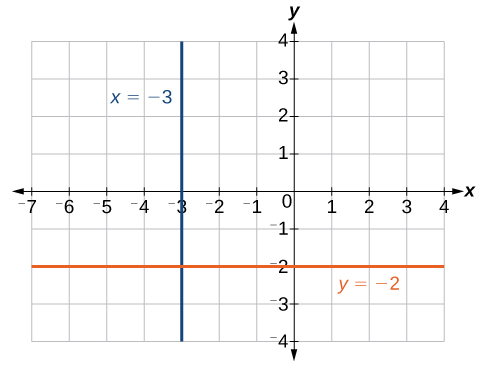
Figure 3. The line x = −3 is a vertical line. The line y = −2 is a horizontal line.
Find the equation of the line passing through the given points: [latex]\\left(1,-3\\right)[/latex] and [latex]\\left(1,4\\right)[/latex].
The x-coordinate of both points is 1. Therefore, we have a vertical line, [latex]x=1[/latex].
Find the equation of the line passing through [latex]\left(-5,2\right)[/latex] and [latex]\left(2,2\right)[/latex].
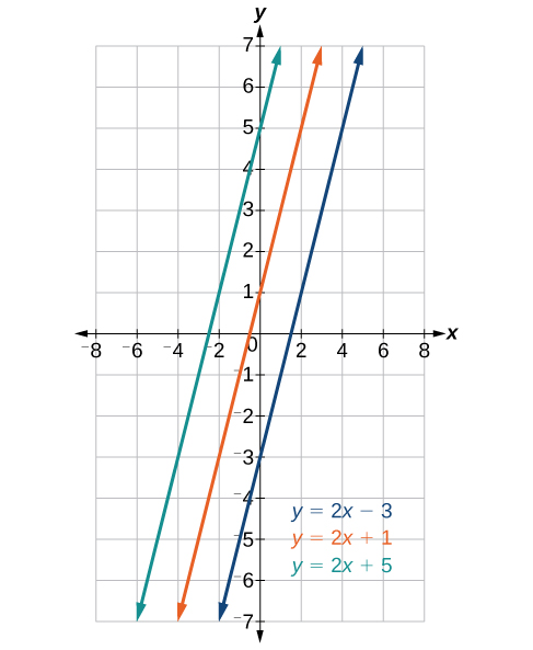
Figure 4. Parallel lines
Parallel lines have the same slope and different y-intercepts. Lines that are parallel to each other will never intersect. For example, Figure 4 shows the graphs of various lines with the same slope, [latex]m=2[/latex].
All of the lines shown in the graph are parallel because they have the same slope and different y-intercepts.
Lines that are perpendicular intersect to form a [latex]{90}^{\circ }[/latex] -angle. The slope of one line is the negative reciprocal of the other. We can show that two lines are perpendicular if the product of the two slopes is [latex]-1:{m}_{1}\cdot {m}_{2}=-1[/latex]. For example, Figure 4 shows the graph of two perpendicular lines. One line has a slope of 3; the other line has a slope of [latex]-\frac{1}{3}[/latex].
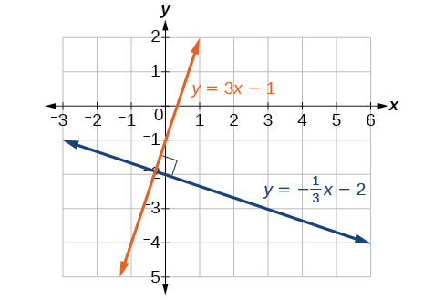
Figure 5. Perpendicular lines
Graph the equations of the given lines, and state whether they are parallel, perpendicular, or neither: [latex]3y=-4x+3[/latex] and [latex]3x - 4y=8[/latex].
The first thing we want to do is rewrite the equations so that both equations are in slope-intercept form.
First equation:
Second equation:
See the graph of both lines in Figure 6.
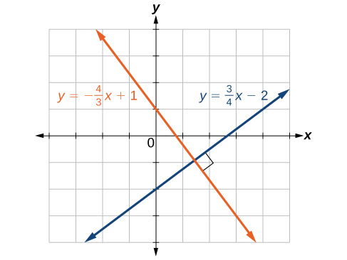
Figure 6
From the graph, we can see that the lines appear perpendicular, but we must compare the slopes.
The slopes are negative reciprocals of each other, confirming that the lines are perpendicular.
Graph the two lines and determine whether they are parallel, perpendicular, or neither: [latex]2y-x=10[/latex] and [latex]2y=x+4[/latex].
As we have learned, determining whether two lines are parallel or perpendicular is a matter of finding the slopes. To write the equation of a line parallel or perpendicular to another line, we follow the same principles as we do for finding the equation of any line. After finding the slope, use the point-slope formula to write the equation of the new line.
Write the equation of line parallel to a [latex]5x+3y=1[/latex] and passing through the point [latex]\left(3,5\right)[/latex].
First, we will write the equation in slope-intercept form to find the slope.
The slope is [latex]m=-\frac{5}{3}[/latex]. The y-intercept is [latex]\frac{1}{3}[/latex], but that really does not enter into our problem, as the only thing we need for two lines to be parallel is the same slope. The one exception is that if the y-intercepts are the same, then the two lines are the same line. The next step is to use this slope and the given point with the point-slope formula.
The equation of the line is [latex]y=-\frac{5}{3}x+10[/latex].
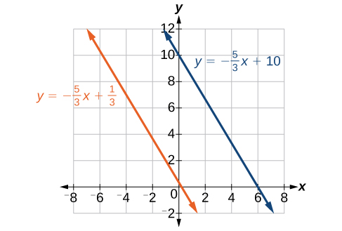
Figure 7
Find the equation of the line parallel to [latex]5x=7+y[/latex] and passing through the point [latex]\left(-1,-2\right)[/latex].
Find the equation of the line perpendicular to [latex]5x - 3y+4=0\left(-4,1\right)[/latex].
The first step is to write the equation in slope-intercept form.
We see that the slope is [latex]m=\frac{5}{3}[/latex]. This means that the slope of the line perpendicular to the given line is the negative reciprocal, or [latex]-\frac{3}{5}[/latex]. Next, we use the point-slope formula with this new slope and the given point.
conditional equation an equation that is true for some values of the variable
identity equation an equation that is true for all values of the variable
inconsistent equation an equation producing a false result
linear equation an algebraic equation in which each term is either a constant or the product of a constant and the first power of a variable
solution set the set of all solutions to an equation
slope the change in y-values over the change in x-values
rational equation an equation consisting of a fraction of polynomials
1. What does it mean when we say that two lines are parallel?
2. What is the relationship between the slopes of perpendicular lines (assuming neither is horizontal nor vertical)?
3. How do we recognize when an equation, for example [latex]y=4x+3[/latex], will be a straight line (linear) when graphed?
4. What does it mean when we say that a linear equation is inconsistent?
5. When solving the following equation: [latex]\frac{2}{x - 5}=\frac{4}{x+1}[/latex], explain why we must exclude [latex]x=5[/latex] and [latex]x=-1[/latex] as possible solutions from the solution set.
For the following exercises, solve the equation for [latex]x[/latex].
6. [latex]7x+2=3x - 9[/latex]
7. [latex]4x - 3=5[/latex]
8. [latex]3\left(x+2\right)-12=5\left(x+1\right)[/latex]
9. [latex]12 - 5\left(x+3\right)=2x - 5[/latex]
10. [latex]\frac{1}{2}-\frac{1}{3}x=\frac{4}{3}[/latex]
11. [latex]\frac{x}{3}-\frac{3}{4}=\frac{2x+3}{12}[/latex]
12. [latex]\frac{2}{3}x+\frac{1}{2}=\frac{31}{6}[/latex]
13. [latex]3\left(2x - 1\right)+x=5x+3[/latex]
14. [latex]\frac{2x}{3}-\frac{3}{4}=\frac{x}{6}+\frac{21}{4}[/latex]
15. [latex]\frac{x+2}{4}-\frac{x - 1}{3}=2[/latex]
For the following exercises, solve each rational equation for [latex]x[/latex]. State all x-values that are excluded from the solution set.
16. [latex]\frac{3}{x}-\frac{1}{3}=\frac{1}{6}[/latex]
17. [latex]2-\frac{3}{x+4}=\frac{x+2}{x+4}[/latex]
18. [latex]\frac{3}{x - 2}=\frac{1}{x - 1}+\frac{7}{\left(x - 1\right)\left(x - 2\right)}[/latex]
19. [latex]\frac{3x}{x - 1}+2=\frac{3}{x - 1}[/latex]
20. [latex]\frac{5}{x+1}+\frac{1}{x - 3}=\frac{-6}{{x}^{2}-2x - 3}[/latex]
21. [latex]\frac{1}{x}=\frac{1}{5}+\frac{3}{2x}[/latex]
For the following exercises, find the equation of the line using the point-slope formula. Write all the final equations using the slope-intercept form.
22. [latex]\left(0,3\right)[/latex] with a slope of [latex]\frac{2}{3}[/latex]
23. [latex]\left(1,2\right)[/latex] with a slope of [latex]\frac{-4}{5}[/latex]
24. x-intercept is 1, and [latex]\left(-2,6\right)[/latex]
25. y-intercept is 2, and [latex]\left(4,-1\right)[/latex]
26. [latex]\left(-3,10\right)[/latex] and [latex]\left(5,-6\right)[/latex]
27. [latex]\left(1,3\right)\text{ and }\left(5,5\right)[/latex]
28. parallel to [latex]y=2x+5[/latex] and passes through the point [latex]\left(4,3\right)[/latex]
29. perpendicular to [latex]\text{3}y=x - 4[/latex] and passes through the point [latex]\left(-2,1\right)[/latex] .
For the following exercises, find the equation of the line using the given information.
30. [latex]\left(-2,0\right)[/latex] and [latex]\left(-2,5\right)[/latex]
31. [latex]\left(1,7\right)[/latex] and [latex]\left(3,7\right)[/latex]
32. The slope is undefined and it passes through the point [latex]\left(2,3\right)[/latex].
33. The slope equals zero and it passes through the point [latex]\left(1,-4\right)[/latex].
34. The slope is [latex]\frac{3}{4}[/latex] and it passes through the point [latex]\left(1,4\right)[/latex].
35. [latex]\left(-1,3\right)[/latex] and [latex]\left(4,-5\right)[/latex]
For the following exercises, graph the pair of equations on the same axes, and state whether they are parallel, perpendicular, or neither.
36. [latex]\begin{array}{l}\\ y=2x+7\hfill \\ y=\frac{-1}{2}x - 4\hfill \end{array}[/latex]
37. [latex]\begin{array}{l}3x - 2y=5\hfill \\ 6y - 9x=6\hfill \end{array}[/latex]
38. [latex]\begin{array}{l}y=\frac{3x+1}{4}\hfill \\ y=3x+2\hfill \end{array}[/latex]
39. [latex]\begin{array}{l}x=4\\ y=-3\end{array}[/latex]
For the following exercises, find the slope of the line that passes through the given points.
40. [latex]\left(5,4\right)[/latex] and [latex]\left(7,9\right)[/latex]
41. [latex]\left(-3,2\right)[/latex] and [latex]\left(4,-7\right)[/latex]
42. [latex]\left(-5,4\right)[/latex] and [latex]\left(2,4\right)[/latex]
43. [latex]\left(-1,-2\right)[/latex] and [latex]\left(3,4\right)[/latex]
44. [latex]\left(3,-2\right)[/latex] and [latex]\left(3,-2\right)[/latex]
For the following exercises, find the slope of the lines that pass through each pair of points and determine whether the lines are parallel or perpendicular.
45. [latex]\begin{array}{l}\left(-1,3\right)\text{ and }\left(5,1\right)\\ \left(-2,3\right)\text{ and }\left(0,9\right)\end{array}[/latex]
46. [latex]\begin{array}{l}\left(2,5\right)\text{ and }\left(5,9\right)\\ \left(-1,-1\right)\text{ and }\left(2,3\right)\end{array}[/latex]
For the following exercises, express the equations in slope intercept form (rounding each number to the thousandths place). Enter this into a graphing calculator as Y1, then adjust the ymin and ymax values for your window to include where the y-intercept occurs. State your ymin and ymax values.
47. [latex]0.537x - 2.19y=100[/latex]
48. [latex]4,500x - 200y=9,528[/latex]
49. [latex]\frac{200 - 30y}{x}=70[/latex]
50. Starting with the point-slope formula [latex]y-{y}_{1}=m\left(x-{x}_{1}\right)[/latex], solve this expression for [latex]x[/latex] in terms of [latex]{x}_{1},y,{y}_{1}[/latex], and [latex]m[/latex].
51. Starting with the standard form of an equation [latex]\text{A}x\text{ + B}y\text{ = C,}[/latex] solve this expression for y in terms of [latex]A,B,C[/latex], and [latex]x[/latex]. Then put the expression in slope-intercept form.
52. Use the above derived formula to put the following standard equation in slope intercept form: [latex]7x - 5y=25[/latex].
53. Given that the following coordinates are the vertices of a rectangle, prove that this truly is a rectangle by showing the slopes of the sides that meet are perpendicular.
54. Find the slopes of the diagonals in the previous exercise. Are they perpendicular?
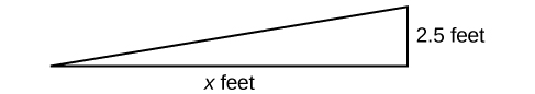
55. The slope for a wheelchair ramp for a home has to be [latex]\frac{1}{12}[/latex]. If the vertical distance from the ground to the door bottom is 2.5 ft, find the distance the ramp has to extend from the home in order to comply with the needed slope.
56. If the profit equation for a small business selling [latex]x[/latex] number of item one and [latex]y[/latex] number of item two is [latex]p=3x+4y[/latex], find the [latex]y[/latex] value when [latex]p=\$453\text{ and }x=75[/latex].
For the following exercises, use this scenario: The cost of renting a car is $45/wk plus $0.25/mi traveled during that week. An equation to represent the cost would be [latex]y=45+.25x[/latex], where [latex]x[/latex] is the number of miles traveled.
57. What is your cost if you travel 50 mi?
58. If your cost were [latex]\$63.75[/latex], how many miles were you charged for traveling?
59. Suppose you have a maximum of $100 to spend for the car rental. What would be the maximum number of miles you could travel?
1. [latex]x=-5[/latex]
2. [latex]x=-3[/latex]
3. [latex]x=\frac{10}{3}[/latex]
4. [latex]x=1[/latex]
5. [latex]x=-\frac{7}{17}[/latex]. Excluded values are [latex]x=-\frac{1}{2}[/latex] and [latex]x=-\frac{1}{3}[/latex].
6. [latex]x=\frac{1}{3}[/latex]
7. [latex]m=-\frac{2}{3}[/latex]
8. [latex]y=4x - 3[/latex]
9. [latex]x+3y=2[/latex]
10. Horizontal line: [latex]y=2[/latex]
11. Parallel lines: equations are written in slope-intercept form.

12. [latex]y=5x+3[/latex]
1. It means they have the same slope.
3. The exponent of the [latex]x[/latex] variable is 1. It is called a first-degree equation.
5. If we insert either value into the equation, they make an expression in the equation undefined (zero in the denominator).
7. [latex]x=2[/latex]
9. [latex]x=\frac{2}{7}[/latex]
11. [latex]x=6[/latex]
13. [latex]x=3[/latex]
15. [latex]x=-14[/latex]
17. [latex]x\ne -4[/latex]; [latex]x=-3[/latex]
19. [latex]x\ne 1[/latex]; when we solve this we get [latex]x=1[/latex], which is excluded, therefore NO solution
21. [latex]x\ne 0[/latex]; [latex]x=\frac{-5}{2}[/latex]
23. [latex]y=\frac{-4}{5}x+\frac{14}{5}[/latex]
25. [latex]y=\frac{-3}{4}x+2[/latex]
27. [latex]y=\frac{1}{2}x+\frac{5}{2}[/latex]
29. [latex]y=-3x - 5[/latex]
31. [latex]y=7[/latex]
33. [latex]y=-4[/latex]
35. [latex]8x+5y=7[/latex]
37. Parallel

39. Perpendicular

41. [latex]m=\frac{-9}{7}[/latex]
43. [latex]m=\frac{3}{2}[/latex]
45. [latex]{m}_{1}=\frac{-1}{3},\text{ }{m}_{2}=3;\text{ }\text{Perpendicular}[/latex]
47. [latex]y=0.245x - 45.662[/latex]. Answers may vary. [latex]{y}_{\text{min}}=-50,\text{ }{y}_{\text{max}}=-40[/latex]
49. [latex]y=-2.333x+6.667[/latex]. Answers may vary. [latex]{y}_{\mathrm{min}}=-10, {y}_{\mathrm{max}}=10[/latex]
51. [latex]y=\frac{-A}{B}x+\frac{C}{B}[/latex]
53. Yes, they are perpendicular.
55. 30 ft
57. $57.50
59. 220 mi
By the end of this section, you will be able to:
Figure 1. Credit: Kevin Dooley
Josh is hoping to get an A in his college algebra class. He has scores of 75, 82, 95, 91, and 94 on his first five tests. Only the final exam remains, and the maximum of points that can be earned is 100. Is it possible for Josh to end the course with an A? A simple linear equation will give Josh his answer.
Many real-world applications can be modeled by linear equations. For example, a cell phone package may include a monthly service fee plus a charge per minute of talk-time; it costs a widget manufacturer a certain amount to produce x widgets per month plus monthly operating charges; a car rental company charges a daily fee plus an amount per mile driven. These are examples of applications we come across every day that are modeled by linear equations. In this section, we will set up and use linear equations to solve such problems.
To set up or model a linear equation to fit a real-world application, we must first determine the known quantities and define the unknown quantity as a variable. Then, we begin to interpret the words as mathematical expressions using mathematical symbols. Let us use the car rental example above. In this case, a known cost, such as $0.10/mi, is multiplied by an unknown quantity, the number of miles driven. Therefore, we can write [latex]0.10x[/latex]. This expression represents a variable cost because it changes according to the number of miles driven.
If a quantity is independent of a variable, we usually just add or subtract it, according to the problem. As these amounts do not change, we call them fixed costs. Consider a car rental agency that charges $0.10/mi plus a daily fee of $50. We can use these quantities to model an equation that can be used to find the daily car rental cost [latex]C[/latex].
When dealing with real-world applications, there are certain expressions that we can translate directly into math. The table lists some common verbal expressions and their equivalent mathematical expressions.
| Verbal | Translation to Math Operations |
|---|---|
| One number exceeds another by a | [latex]x,\text{ }x+a[/latex] |
| Twice a number | [latex]2x[/latex] |
| One number is a more than another number | [latex]x,\text{ }x+a[/latex] |
| One number is a less than twice another number | [latex]x,2x-a[/latex] |
| The product of a number and a, decreased by b | [latex]ax-b[/latex] |
| The quotient of a number and the number plus a is three times the number | [latex]\frac{x}{x+a}=3x[/latex] |
| The product of three times a number and the number decreased by b is c | [latex]3x\left(x-b\right)=c[/latex] |
Find a linear equation to solve for the following unknown quantities: One number exceeds another number by [latex]17[/latex] and their sum is [latex]31[/latex]. Find the two numbers.
Let [latex]x[/latex] equal the first number. Then, as the second number exceeds the first by 17, we can write the second number as [latex]x+17[/latex]. The sum of the two numbers is 31. We usually interpret the word is as an equal sign.
The two numbers are [latex]7[/latex] and [latex]24[/latex].
Find a linear equation to solve for the following unknown quantities: One number is three more than twice another number. If the sum of the two numbers is [latex]36[/latex], find the numbers.
There are two cell phone companies that offer different packages. Company A charges a monthly service fee of $34 plus $.05/min talk-time. Company B charges a monthly service fee of $40 plus $.04/min talk-time.
So, Company B offers the lower monthly cost of $86.40 as compared with the $92 monthly cost offered by Company A when the average number of minutes used each month is 1,160.
If the average number of minutes used each month is 420, then Company A offers a lower monthly cost of $55 compared to Company B’s monthly cost of $56.80.
Check the x-value in each equation.
Therefore, a monthly average of 600 talk-time minutes renders the plans equal.
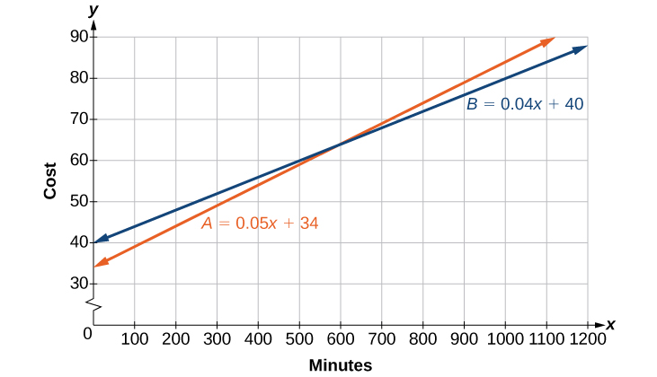
Figure 2
Find a linear equation to model this real-world application: It costs ABC electronics company $2.50 per unit to produce a part used in a popular brand of desktop computers. The company has monthly operating expenses of $350 for utilities and $3,300 for salaries. What are the company’s monthly expenses?
Many applications are solved using known formulas. The problem is stated, a formula is identified, the known quantities are substituted into the formula, the equation is solved for the unknown, and the problem’s question is answered. Typically, these problems involve two equations representing two trips, two investments, two areas, and so on. Examples of formulas include the area of a rectangular region, [latex]A=LW[/latex]; the perimeter of a rectangle, [latex]P=2L+2W[/latex]; and the volume of a rectangular solid, [latex]V=LWH[/latex]. When there are two unknowns, we find a way to write one in terms of the other because we can solve for only one variable at a time.
It takes Andrew 30 min to drive to work in the morning. He drives home using the same route, but it takes 10 min longer, and he averages 10 mi/h less than in the morning. How far does Andrew drive to work?
This is a distance problem, so we can use the formula [latex]d=rt[/latex], where distance equals rate multiplied by time. Note that when rate is given in mi/h, time must be expressed in hours. Consistent units of measurement are key to obtaining a correct solution.
First, we identify the known and unknown quantities. Andrew’s morning drive to work takes 30 min, or [latex]\frac{1}{2}[/latex] h at rate [latex]r[/latex]. His drive home takes 40 min, or [latex]\frac{2}{3}[/latex] h, and his speed averages 10 mi/h less than the morning drive. Both trips cover distance [latex]d[/latex]. A table, such as the one below, is often helpful for keeping track of information in these types of problems.
| [latex]d[/latex] | [latex]r[/latex] | [latex]t[/latex] | |
|---|---|---|---|
| To Work | [latex]d[/latex] | [latex]r[/latex] | [latex]\frac{1}{2}[/latex] |
| To Home | [latex]d[/latex] | [latex]r - 10[/latex] | [latex]\frac{2}{3}[/latex] |
Write two equations, one for each trip.
As both equations equal the same distance, we set them equal to each other and solve for r.
We have solved for the rate of speed to work, 40 mph. Substituting 40 into the rate on the return trip yields 30 mi/h. Now we can answer the question. Substitute the rate back into either equation and solve for d.
The distance between home and work is 20 mi.
Note that we could have cleared the fractions in the equation by multiplying both sides of the equation by the LCD to solve for [latex]r[/latex].
On Saturday morning, it took Jennifer 3.6 h to drive to her mother’s house for the weekend. On Sunday evening, due to heavy traffic, it took Jennifer 4 h to return home. Her speed was 5 mi/h slower on Sunday than on Saturday. What was her speed on Sunday?
The perimeter of a rectangular outdoor patio is [latex]54[/latex] ft. The length is [latex]3[/latex] ft greater than the width. What are the dimensions of the patio?
The perimeter formula is standard: [latex]P=2L+2W[/latex]. We have two unknown quantities, length and width. However, we can write the length in terms of the width as [latex]L=W+3[/latex]. Substitute the perimeter value and the expression for length into the formula. It is often helpful to make a sketch and label the sides.
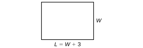
Figure 3
Now we can solve for the width and then calculate the length.
The dimensions are [latex]L=15[/latex] ft and [latex]W=12[/latex] ft.
Find the dimensions of a rectangle given that the perimeter is [latex]110[/latex] cm and the length is 1 cm more than twice the width.
The perimeter of a tablet of graph paper is 48 in2. The length is [latex]6[/latex] in. more than the width. Find the area of the graph paper.
The standard formula for area is [latex]A=LW[/latex]; however, we will solve the problem using the perimeter formula. The reason we use the perimeter formula is because we know enough information about the perimeter that the formula will allow us to solve for one of the unknowns. As both perimeter and area use length and width as dimensions, they are often used together to solve a problem such as this one.
We know that the length is 6 in. more than the width, so we can write length as [latex]L=W+6[/latex]. Substitute the value of the perimeter and the expression for length into the perimeter formula and find the length.
Now, we find the area given the dimensions of [latex]L=15[/latex] in. and [latex]W=9[/latex] in.
The area is [latex]135[/latex] in2.
A game room has a perimeter of 70 ft. The length is five more than twice the width. How many ft2 of new carpeting should be ordered?
Find the dimensions of a shipping box given that the length is twice the width, the height is [latex]8[/latex] inches, and the volume is 1,600 in.3.
The formula for the volume of a box is given as [latex]V=LWH[/latex], the product of length, width, and height. We are given that [latex]L=2W[/latex], and [latex]H=8[/latex]. The volume is [latex]1,600[/latex] cubic inches.
The dimensions are [latex]L=20[/latex] in., [latex]W=10[/latex] in., and [latex]H=8[/latex] in.
Note that the square root of [latex]{W}^{2}[/latex] would result in a positive and a negative value. However, because we are describing width, we can use only the positive result.
area in square units, the area formula used in this section is used to find the area of any two-dimensional rectangular region: [latex]A=LW[/latex]
perimeter in linear units, the perimeter formula is used to find the linear measurement, or outside length and width, around a two-dimensional regular object; for a rectangle: [latex]P=2L+2W[/latex]
volume in cubic units, the volume measurement includes length, width, and depth: [latex]V=LWH[/latex]
1. To set up a model linear equation to fit real-world applications, what should always be the first step?
2. Use your own words to describe this equation where n is a number:
3. If the total amount of money you had to invest was $2,000 and you deposit [latex]x[/latex] amount in one investment, how can you represent the remaining amount?
4. If a man sawed a 10-ft board into two sections and one section was [latex]n[/latex] ft long, how long would the other section be in terms of [latex]n[/latex] ?
5. If Bill was traveling [latex]v[/latex] mi/h, how would you represent Daemon’s speed if he was traveling 10 mi/h faster?
For the following exercises, use the information to find a linear algebraic equation model to use to answer the question being asked.
6. Mark and Don are planning to sell each of their marble collections at a garage sale. If Don has 1 more than 3 times the number of marbles Mark has, how many does each boy have to sell if the total number of marbles is 113?
7. Beth and Ann are joking that their combined ages equal Sam’s age. If Beth is twice Ann’s age and Sam is 69 yr old, what are Beth and Ann’s ages?
8. Ben originally filled out 8 more applications than Henry. Then each boy filled out 3 additional applications, bringing the total to 28. How many applications did each boy originally fill out?
For the following exercises, use this scenario: Two different telephone carriers offer the following plans that a person is considering. Company A has a monthly fee of $20 and charges of $.05/min for calls. Company B has a monthly fee of $5 and charges $.10/min for calls.
9. Find the model of the total cost of Company A’s plan, using [latex]m[/latex] for the minutes.
10. Find the model of the total cost of Company B’s plan, using [latex]m[/latex] for the minutes.
11. Find out how many minutes of calling would make the two plans equal.
12. If the person makes a monthly average of 200 min of calls, which plan should for the person choose?
For the following exercises, use this scenario: A wireless carrier offers the following plans that a person is considering. The Family Plan: $90 monthly fee, unlimited talk and text on up to 5 lines, and data charges of $40 for each device for up to 2 GB of data per device. The Mobile Share Plan: $120 monthly fee for up to 10 devices, unlimited talk and text for all the lines, and data charges of $35 for each device up to a shared total of 10 GB of data. Use [latex]P[/latex] for the number of devices that need data plans as part of their cost.
13. Find the model of the total cost of the Family Plan.
14. Find the model of the total cost of the Mobile Share Plan.
15. Assuming they stay under their data limit, find the number of devices that would make the two plans equal in cost.
16. If a family has 3 smart phones, which plan should they choose?
For exercises 17 and 18, use this scenario: A retired woman has $50,000 to invest but needs to make $6,000 a year from the interest to meet certain living expenses. One bond investment pays 15% annual interest. The rest of it she wants to put in a CD that pays 7%.
17. If we let [latex]x[/latex] be the amount the woman invests in the 15% bond, how much will she be able to invest in the CD?
18. Set up and solve the equation for how much the woman should invest in each option to sustain a $6,000 annual return.
19. Two planes fly in opposite directions. One travels 450 mi/h and the other 550 mi/h. How long will it take before they are 4,000 mi apart?
20. Ben starts walking along a path at 4 mi/h. One and a half hours after Ben leaves, his sister Amanda begins jogging along the same path at 6 mi/h. How long will it be before Amanda catches up to Ben?
21. Fiora starts riding her bike at 20 mi/h. After a while, she slows down to 12 mi/h, and maintains that speed for the rest of the trip. The whole trip of 70 mi takes her 4.5 h. For what distance did she travel at 20 mi/h?
22. A chemistry teacher needs to mix a 30% salt solution with a 70% salt solution to make 20 qt of a 40% salt solution. How many quarts of each solution should the teacher mix to get the desired result?
23. Paul has $20,000 to invest. His intent is to earn 11% interest on his investment. He can invest part of his money at 8% interest and part at 12% interest. How much does Paul need to invest in each option to make get a total 11% return on his $20,000?
For the following exercises, use this scenario: A truck rental agency offers two kinds of plans. Plan A charges $75/wk plus $.10/mi driven. Plan B charges $100/wk plus $.05/mi driven.
24. Write the model equation for the cost of renting a truck with plan A.
25. Write the model equation for the cost of renting a truck with plan B.
26. Find the number of miles that would generate the same cost for both plans.
27. If Tim knows he has to travel 300 mi, which plan should he choose?
For the following exercises, use the given formulas to answer the questions.
28. [latex]A=P\left(1+rt\right)[/latex] is used to find the principal amount P deposited, earning r% interest, for t years. Use this to find what principal amount P David invested at a 3% rate for 20 yr if [latex]A=\$8,000[/latex].
29. The formula [latex]F=\frac{m{v}^{2}}{R}[/latex] relates force (F), velocity (v), mass (m), and resistance (R). Find [latex]R[/latex] when [latex]m=45[/latex], [latex]v=7[/latex], and [latex]F=245[/latex].
30. [latex]F=ma[/latex] indicates that force (F) equals mass (m) times acceleration (a). Find the acceleration of a mass of 50 kg if a force of 12 N is exerted on it.
31. [latex]Sum=\frac{1}{1-r}[/latex] is the formula for an infinite series sum. If the sum is 5, find [latex]r[/latex].
For the following exercises, solve for the given variable in the formula. After obtaining a new version of the formula, you will use it to solve a question.
32. Solve for W: [latex]P=2L+2W[/latex]
33. Use the formula from the previous question to find the width, [latex]W[/latex], of a rectangle whose length is 15 and whose perimeter is 58.
34. Solve for [latex]f:\frac{1}{p}+\frac{1}{q}=\frac{1}{f}[/latex]
35. Use the formula from the previous question to find [latex]f[/latex] when [latex]p=8\text{and }q=13[/latex].
36. Solve for [latex]m[/latex] in the slope-intercept formula: [latex]y=mx+b[/latex]
37. Use the formula from the previous question to find [latex]m[/latex] when the coordinates of the point are [latex]\left(4,7\right)[/latex] and [latex]b=12[/latex].
38. The area of a trapezoid is given by [latex]A=\frac{1}{2}h\left({b}_{1}+{b}_{2}\right)[/latex]. Use the formula to find the area of a trapezoid with [latex]h=6,\text{ }{b}_{1}=14,\text{ and }{b}_{2}=8[/latex].
39. Solve for h: [latex]A=\frac{1}{2}h\left({b}_{1}+{b}_{2}\right)[/latex]
40. Use the formula from the previous question to find the height of a trapezoid with [latex]A=150,\text{ }{b}_{1}=19,\text{ and }{b}_{2}=11[/latex].
41. Find the dimensions of an American football field. The length is 200 ft more than the width, and the perimeter is 1,040 ft. Find the length and width. Use the perimeter formula [latex]P=2L+2W[/latex].
42. Distance equals rate times time, [latex]d=rt[/latex]. Find the distance Tom travels if he is moving at a rate of 55 mi/h for 3.5 h.
43. Using the formula in the previous exercise, find the distance that Susan travels if she is moving at a rate of 60 mi/h for 6.75 h.
44. What is the total distance that two people travel in 3 h if one of them is riding a bike at 15 mi/h and the other is walking at 3 mi/h?
45. If the area model for a triangle is [latex]A=\frac{1}{2}bh[/latex], find the area of a triangle with a height of 16 in. and a base of 11 in.
46. Solve for h: [latex]A=\frac{1}{2}bh[/latex]
47. Use the formula from the previous question to find the height to the nearest tenth of a triangle with a base of 15 and an area of 215.
48. The volume formula for a cylinder is [latex]V=\pi {r}^{2}h[/latex]. Using the symbol [latex]\pi [/latex] in your answer, find the volume of a cylinder with a radius, [latex]r[/latex], of 4 cm and a height of 14 cm.
49. Solve for h: [latex]V=\pi {r}^{2}h[/latex]
50. Use the formula from the previous question to find the height of a cylinder with a radius of 8 and a volume of [latex]16\pi [/latex]
51. Solve for r: [latex]V=\pi {r}^{2}h[/latex]
52. Use the formula from the previous question to find the radius of a cylinder with a height of 36 and a volume of [latex]324\pi [/latex].
53. The formula for the circumference of a circle is [latex]C=2\pi r[/latex]. Find the circumference of a circle with a diameter of 12 in. (diameter = 2r). Use the symbol [latex]\pi [/latex] in your final answer.
54. Solve the formula from the previous question for [latex]\pi [/latex]. Notice why [latex]\pi [/latex] is sometimes defined as the ratio of the circumference to its diameter.
1. 11 and 25
2. [latex]C=2.5x+3,650[/latex]
3. 45 mi/h
4. [latex]L=37[/latex] cm, [latex]W=18[/latex] cm
5. 250 ft2
1. Answers may vary. Possible answers: We should define in words what our variable is representing. We should declare the variable. A heading.
3. [latex]2,000-x[/latex]
5. [latex]v+10[/latex]
7. Ann: [latex]23[/latex]; Beth: [latex]46[/latex]
9. [latex]20+0.05m[/latex]
11. 300 min
13. [latex]90+40P[/latex]
15. 6 devices
17. [latex]50,000-x[/latex]
19. 4 h
21. She traveled for 2 h at 20 mi/h, or 40 miles.
23. $5,000 at 8% and $15,000 at 12%
25. [latex]B=100+.05x[/latex]
27. Plan A
29. [latex]R=9[/latex]
31. [latex]r=\frac{4}{5}[/latex] or 0.8
33. [latex]W=\frac{P - 2L}{2}=\frac{58 - 2\left(15\right)}{2}=14[/latex]
35. [latex]f=\frac{pq}{p+q}=\frac{8\left(13\right)}{8+13}=\frac{104}{21}[/latex]
37. [latex]m=\frac{-5}{4}[/latex]
39. [latex]h=\frac{2A}{{b}_{1}+{b}_{2}}[/latex]
41. length = 360 ft; width = 160 ft
43. 405 mi
45. [latex]A=88\text{ in}{.}^{2}[/latex]
47. 28.7
49. [latex]h=\frac{V}{\pi {r}^{2}}[/latex]
51. [latex]r=\sqrt{\frac{V}{\pi h}}[/latex]
53. [latex]C=12\pi [/latex]
By the end of this lesson, you will be able to:
The study of mathematics continuously builds upon itself. Negative integers, for example, fill a void left by the set of positive integers. The set of rational numbers, in turn, fills a void left by the set of integers. The set of real numbers fills a void left by the set of rational numbers. Not surprisingly, the set of real numbers has voids as well. For example, we still have no solution to equations such as
Our best guesses might be +2 or –2. But if we test +2 in this equation, it does not work. If we test –2, it does not work. If we want to have a solution for this equation, we will have to go farther than we have so far. After all, to this point we have described the square root of a negative number as undefined. Fortunately, there is another system of numbers that provides solutions to problems such as these. In this section, we will explore this number system and how to work within it.
We know how to find the square root of any positive real number. In a similar way, we can find the square root of a negative number. The difference is that the root is not real. If the value in the radicand is negative, the root is said to be an imaginary number. The imaginary number [latex]i[/latex] is defined as the square root of negative 1.
So, using properties of radicals,
We can write the square root of any negative number as a multiple of i. Consider the square root of –25.
We use 5i and not [latex]-\text{5}i\\[/latex] because the principal root of 25 is the positive root.

Figure 1
A complex number is the sum of a real number and an imaginary number. A complex number is expressed in standard form when written a + bi where a is the real part and bi is the imaginary part. For example, [latex]5+2i\\[/latex] is a complex number. So, too, is [latex]3+4\sqrt{3}i\\[/latex].
Imaginary numbers are distinguished from real numbers because a squared imaginary number produces a negative real number. Recall, when a positive real number is squared, the result is a positive real number and when a negative real number is squared, again, the result is a positive real number. Complex numbers are a combination of real and imaginary numbers.
A complex number is a number of the form [latex]a+bi\\[/latex] where
If [latex]b=0\\[/latex], then [latex]a+bi\\[/latex] is a real number. If [latex]a=0\\[/latex] and b is not equal to 0, the complex number is called an imaginary number. An imaginary number is an even root of a negative number.
How To: Given an imaginary number, express it in standard form.
Express [latex]\sqrt{-9}\\[/latex] in standard form.
[latex]\sqrt{-9}=\sqrt{9}\sqrt{-1}=3i\\[/latex]
In standard form, this is [latex]0+3i\\[/latex].
We cannot plot complex numbers on a number line as we might real numbers. However, we can still represent them graphically. To represent a complex number we need to address the two components of the number. We use the complex plane, which is a coordinate system in which the horizontal axis represents the real component and the vertical axis represents the imaginary component. Complex numbers are the points on the plane, expressed as ordered pairs (a, b), where a represents the coordinate for the horizontal axis and b represents the coordinate for the vertical axis.
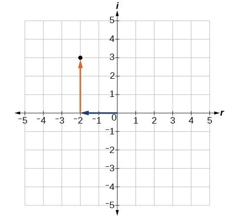
Figure 2
Let’s consider the number [latex]-2+3i\\[/latex]. The real part of the complex number is –2 and the imaginary part is 3i. We plot the ordered pair [latex]\left(-2,3\right)\\[/latex] to represent the complex number [latex]-2+3i\\[/latex].
Figure 3
In the complex plane, the horizontal axis is the real axis, and the vertical axis is the imaginary axis.
Plot the complex number [latex]3 - 4i\\[/latex] on the complex plane.
The real part of the complex number is 3, and the imaginary part is –4i. We plot the ordered pair [latex]\left(3,-4\right)\\[/latex].
Figure 4
Just as with real numbers, we can perform arithmetic operations on complex numbers. To add or subtract complex numbers, we combine the real parts and combine the imaginary parts.
Adding complex numbers:
Subtracting complex numbers:
Add [latex]3 - 4i\\[/latex] and [latex]2+5i\\[/latex].
We add the real parts and add the imaginary parts.
Multiplying complex numbers is much like multiplying binomials. The major difference is that we work with the real and imaginary parts separately.
Figure 5
Let’s begin by multiplying a complex number by a real number. We distribute the real number just as we would with a binomial. So, for example,
Find the product [latex]4\left(2+5i\right)\\[/latex].
Distribute the 4.
Now, let’s multiply two complex numbers. We can use either the distributive property or the FOIL method. Recall that FOIL is an acronym for multiplying First, Outer, Inner, and Last terms together. Using either the distributive property or the FOIL method, we get
Because [latex]{i}^{2}=-1\\[/latex], we have
To simplify, we combine the real parts, and we combine the imaginary parts.
Multiply [latex]\left(4+3i\right)\left(2 - 5i\right)\\[/latex].
Use [latex]\left(a+bi\right)\left(c+di\right)=\left(ac-bd\right)+\left(ad+bc\right)i\\[/latex]
https://youtu.be/O9xQaIi0NX0
Division of two complex numbers is more complicated than addition, subtraction, and multiplication because we cannot divide by an imaginary number, meaning that any fraction must have a real-number denominator. We need to find a term by which we can multiply the numerator and the denominator that will eliminate the imaginary portion of the denominator so that we end up with a real number as the denominator. This term is called the complex conjugate of the denominator, which is found by changing the sign of the imaginary part of the complex number. In other words, the complex conjugate of [latex]a+bi\\[/latex] is [latex]a-bi\\[/latex].
Note that complex conjugates have a reciprocal relationship: The complex conjugate of [latex]a+bi\\[/latex] is [latex]a-bi\\[/latex], and the complex conjugate of [latex]a-bi\\[/latex] is [latex]a+bi\\[/latex]. Further, when a quadratic equation with real coefficients has complex solutions, the solutions are always complex conjugates of one another.
Suppose we want to divide [latex]c+di\\[/latex] by [latex]a+bi\\[/latex], where neither a nor b equals zero. We first write the division as a fraction, then find the complex conjugate of the denominator, and multiply.
Multiply the numerator and denominator by the complex conjugate of the denominator.
Apply the distributive property.
Simplify, remembering that [latex]{i}^{2}=-1\\[/latex].
The complex conjugate of a complex number [latex]a+bi\\[/latex] is [latex]a-bi\\[/latex]. It is found by changing the sign of the imaginary part of the complex number. The real part of the number is left unchanged.
Find the complex conjugate of each number.
Divide [latex]\left(2+5i\right)\\[/latex] by [latex]\left(4-i\right)\\[/latex].
We begin by writing the problem as a fraction.
Then we multiply the numerator and denominator by the complex conjugate of the denominator.
To multiply two complex numbers, we expand the product as we would with polynomials (the process commonly called FOIL).
Note that this expresses the quotient in standard form.
Let [latex]f\left(x\right)={x}^{2}-5x+2\\[/latex]. Evaluate [latex]f\left(3+i\right)\\[/latex].
Figure 6
Substitute [latex]x=3+i\\[/latex] into the function [latex]f\left(x\right)={x}^{2}-5x+2\\[/latex] and simplify.
We write [latex]f\left(3+i\right)=-5+i\\[/latex]. Notice that the input is [latex]3+i\\[/latex] and the output is [latex]-5+i\\[/latex].
Let [latex]f\left(x\right)=2{x}^{2}-3x\\[/latex]. Evaluate [latex]f\left(8-i\right)\\[/latex].
Let [latex]f\left(x\right)=\frac{2+x}{x+3}\\[/latex]. Evaluate [latex]f\left(10i\right)\\[/latex].
Substitute [latex]x=10i\\[/latex] and simplify.
Let [latex]f\left(x\right)=\frac{x+1}{x - 4}\\[/latex]. Evaluate [latex]f\left(-i\right)\\[/latex].
The powers of i are cyclic. Let’s look at what happens when we raise i to increasing powers.
We can see that when we get to the fifth power of i, it is equal to the first power. As we continue to multiply i by itself for increasing powers, we will see a cycle of 4. Let’s examine the next 4 powers of i.
Evaluate [latex]{i}^{35}\\[/latex].
Since [latex]{i}^{4}=1\\[/latex], we can simplify the problem by factoring out as many factors of [latex]{i}^{4}\\[/latex] as possible. To do so, first determine how many times 4 goes into 35: [latex]35=4\cdot 8+3\\[/latex].
Can we write [latex]{i}^{35}\\[/latex] in other helpful ways?
As we saw in Example 11, we reduced [latex]{i}^{35}\\[/latex] to [latex]{i}^{3}\\[/latex] by dividing the exponent by 4 and using the remainder to find the simplified form. But perhaps another factorization of [latex]{i}^{35}\\[/latex] may be more useful. The table below shows some other possible factorizations.
| Factorization of [latex]{i}^{35}[/latex] | [latex]{i}^{34}\cdot i\\[/latex] | [latex]{i}^{33}\cdot {i}^{2}\\[/latex] | [latex]{i}^{31}\cdot {i}^{4}\\[/latex] | [latex]{i}^{19}\cdot {i}^{16}\\[/latex] |
| Reduced form | [latex]{\left({i}^{2}\right)}^{17}\cdot i\\[/latex] | [latex]{i}^{33}\cdot \left(-1\right)\\[/latex] | [latex]{i}^{31}\cdot 1\\[/latex] | [latex]{i}^{19}\cdot {\left({i}^{4}\right)}^{4}\\[/latex] |
| Simplified form | [latex]{\left(-1\right)}^{17}\cdot i\\[/latex] | [latex]-{i}^{33}\\[/latex] | [latex]{i}^{31}\\[/latex] | [latex]{i}^{19}\\[/latex] |
Each of these will eventually result in the answer we obtained above but may require several more steps than our earlier method.
1. Explain how to add complex numbers.
2. What is the basic principle in multiplication of complex numbers?
3. Give an example to show the product of two imaginary numbers is not always imaginary.
4. What is a characteristic of the plot of a real number in the complex plane?
For the following exercises, evaluate the algebraic expressions.
5. [latex]\text{If }f\left(x\right)={x}^{2}+x - 4\\[/latex], evaluate [latex]f\left(2i\right)\\[/latex].
6. [latex]\text{If }f\left(x\right)={x}^{3}-2\\[/latex], evaluate [latex]f\left(i\right)\\[/latex].
7. [latex]\text{If }f\left(x\right)={x}^{2}+3x+5\\[/latex], evaluate [latex]f\left(2+i\right)\\[/latex].
8. [latex]\text{If }f\left(x\right)=2{x}^{2}+x - 3\\[/latex], evaluate [latex]f\left(2 - 3i\right)\\[/latex].
9. [latex]\text{If }f\left(x\right)=\frac{x+1}{2-x}\\[/latex], evaluate [latex]f\left(5i\right)\\[/latex].
10. [latex]\text{If }f\left(x\right)=\frac{1+2x}{x+3}\\[/latex], evaluate [latex]f\left(4i\right)\\[/latex].
For the following exercises, determine the number of real and nonreal solutions for each quadratic function shown.
11.
12.
For the following exercises, plot the complex numbers on the complex plane.
13. [latex]1 - 2i\\[/latex]
14. [latex]-2+3i\\[/latex]
15. i
16. [latex]-3 - 4i\\[/latex]
For the following exercises, perform the indicated operation and express the result as a simplified complex number.
17. [latex]\left(3+2i\right)+\left(5 - 3i\right)\\[/latex]
18. [latex]\left(-2 - 4i\right)+\left(1+6i\right)\\[/latex]
19. [latex]\left(-5+3i\right)-\left(6-i\right)\\[/latex]
20. [latex]\left(2 - 3i\right)-\left(3+2i\right)\\[/latex]
21. [latex]\left(-4+4i\right)-\left(-6+9i\right)\\[/latex]
22. [latex]\left(2+3i\right)\left(4i\right)\\[/latex]
23. [latex]\left(5 - 2i\right)\left(3i\right)\\[/latex]
24. [latex]\left(6 - 2i\right)\left(5\right)\\[/latex]
25. [latex]\left(-2+4i\right)\left(8\right)\\[/latex]
26. [latex]\left(2+3i\right)\left(4-i\right)\\[/latex]
27. [latex]\left(-1+2i\right)\left(-2+3i\right)\\[/latex]
28. [latex]\left(4 - 2i\right)\left(4+2i\right)\\[/latex]
29. [latex]\left(3+4i\right)\left(3 - 4i\right)\\[/latex]
30. [latex]\frac{3+4i}{2}\\[/latex]
31. [latex]\frac{6 - 2i}{3}\\[/latex]
32. [latex]\frac{-5+3i}{2i}\\[/latex]
33. [latex]\frac{6+4i}{i}\\[/latex]
34. [latex]\frac{2 - 3i}{4+3i}\\[/latex]
35. [latex]\frac{3+4i}{2-i}\\[/latex]
36. [latex]\frac{2+3i}{2 - 3i}\\[/latex]
37. [latex]\sqrt{-9}+3\sqrt{-16}\\[/latex]
38. [latex]-\sqrt{-4}-4\sqrt{-25}\\[/latex]
39. [latex]\frac{2+\sqrt{-12}}{2}\\[/latex]
40. [latex]\frac{4+\sqrt{-20}}{2}\\[/latex]
41. [latex]{i}^{8}\\[/latex]
42. [latex]{i}^{15}\\[/latex]
43. [latex]{i}^{22}\\[/latex]
For the following exercises, use a calculator to help answer the questions.
44. Evaluate [latex]{\left(1+i\right)}^{k}\\[/latex] for [latex]k=\text{4, 8, and 12}\text{.}\\[/latex] Predict the value if [latex]k=16\\[/latex].
45. Evaluate [latex]{\left(1-i\right)}^{k}\\[/latex] for [latex]k=\text{2, 6, and 10}\text{.}\\[/latex] Predict the value if [latex]k=14\\[/latex].
46. Evaluate [latex]\left(1+i\right)^{k}-\left(1-i\right)^{k}\\[/latex] for [latex]k=\text{4, 8, and 12}\\[/latex]. Predict the value for [latex]k=16\\[/latex].
47. Show that a solution of [latex]{x}^{6}+1=0\\[/latex] is [latex]\frac{\sqrt{3}}{2}+\frac{1}{2}i\\[/latex].
48. Show that a solution of [latex]{x}^{8}-1=0\\[/latex] is [latex]\frac{\sqrt{2}}{2}+\frac{\sqrt{2}}{2}i\\[/latex].
For the following exercises, evaluate the expressions, writing the result as a simplified complex number.
49. [latex]\frac{1}{i}+\frac{4}{{i}^{3}}\\[/latex]
50. [latex]\frac{1}{{i}^{11}}-\frac{1}{{i}^{21}}\\[/latex]
51. [latex]{i}^{7}\left(1+{i}^{2}\right)\\[/latex]
52. [latex]{i}^{-3}+5{i}^{7}\\[/latex]
53. [latex]\frac{\left(2+i\right)\left(4 - 2i\right)}{\left(1+i\right)}\\[/latex]
54. [latex]\frac{\left(1+3i\right)\left(2 - 4i\right)}{\left(1+2i\right)}\\[/latex]
55. [latex]\frac{{\left(3+i\right)}^{2}}{{\left(1+2i\right)}^{2}}\\[/latex]
56. [latex]\frac{3+2i}{2+i}+\left(4+3i\right)\\[/latex]
57. [latex]\frac{4+i}{i}+\frac{3 - 4i}{1-i}\\[/latex]
58. [latex]\frac{3+2i}{1+2i}-\frac{2 - 3i}{3+i}\\[/latex]
By the end of this section, you will be able to:

Figure 1
The computer monitor on the left in Figure 1 is a 23.6-inch model and the one on the right is a 27-inch model. Proportionally, the monitors appear very similar. If there is a limited amount of space and we desire the largest monitor possible, how do we decide which one to choose? In this section, we will learn how to solve problems such as this using four different methods.
An equation containing a second-degree polynomial is called a quadratic equation. For example, equations such as [latex]2{x}^{2}+3x - 1=0[/latex] and [latex]{x}^{2}-4=0[/latex] are quadratic equations. They are used in countless ways in the fields of engineering, architecture, finance, biological science, and, of course, mathematics.
Often the easiest method of solving a quadratic equation is factoring. Factoring means finding expressions that can be multiplied together to give the expression on one side of the equation.
If a quadratic equation can be factored, it is written as a product of linear terms. Solving by factoring depends on the zero-product property, which states that if [latex]a\cdot b=0[/latex], then [latex]a=0[/latex] or [latex]b=0[/latex], where a and b are real numbers or algebraic expressions. In other words, if the product of two numbers or two expressions equals zero, then one of the numbers or one of the expressions must equal zero because zero multiplied by anything equals zero.
Multiplying the factors expands the equation to a string of terms separated by plus or minus signs. So, in that sense, the operation of multiplication undoes the operation of factoring. For example, expand the factored expression [latex]\left(x - 2\right)\left(x+3\right)[/latex] by multiplying the two factors together.
The product is a quadratic expression. Set equal to zero, [latex]{x}^{2}+x - 6=0[/latex] is a quadratic equation. If we were to factor the equation, we would get back the factors we multiplied.
The process of factoring a quadratic equation depends on the leading coefficient, whether it is 1 or another integer. We will look at both situations; but first, we want to confirm that the equation is written in standard form, [latex]a{x}^{2}+bx+c=0[/latex], where a, b, and c are real numbers, and [latex]a\ne 0[/latex]. The equation [latex]{x}^{2}+x - 6=0[/latex] is in standard form.
We can use the zero-product property to solve quadratic equations in which we first have to factor out the greatest common factor (GCF), and for equations that have special factoring formulas as well, such as the difference of squares, both of which we will see later in this section.
The zero-product property states
where a and b are real numbers or algebraic expressions.
A quadratic equation is an equation containing a second-degree polynomial; for example
where a, b, and c are real numbers, and if [latex]a\ne 0[/latex], it is in standard form.
In the quadratic equation [latex]{x}^{2}+x - 6=0[/latex], the leading coefficient, or the coefficient of [latex]{x}^{2}[/latex], is 1. We have one method of factoring quadratic equations in this form.
Factor and solve the equation: [latex]{x}^{2}+x - 6=0[/latex].
To factor [latex]{x}^{2}+x - 6=0[/latex], we look for two numbers whose product equals [latex]-6[/latex] and whose sum equals 1. Begin by looking at the possible factors of [latex]-6[/latex].
The last pair, [latex]3\cdot \left(-2\right)[/latex] sums to 1, so these are the numbers. Note that only one pair of numbers will work. Then, write the factors.
To solve this equation, we use the zero-product property. Set each factor equal to zero and solve.
The two solutions are [latex]x=2[/latex] and [latex]x=-3[/latex]. We can see how the solutions relate to the graph in Figure 2. The solutions are the x-intercepts of [latex]{x}^{2}+x - 6=0[/latex].
Figure 2
Solve the quadratic equation by factoring: [latex]{x}^{2}+8x+15=0[/latex].
Find two numbers whose product equals [latex]15[/latex] and whose sum equals [latex]8[/latex]. List the factors of [latex]15[/latex].
The numbers that add to 8 are 3 and 5. Then, write the factors, set each factor equal to zero, and solve.
The solutions are [latex]x=-3[/latex] and [latex]x=-5[/latex].
Solve the difference of squares equation using the zero-product property: [latex]{x}^{2}-9=0[/latex].
Recognizing that the equation represents the difference of squares, we can write the two factors by taking the square root of each term, using a minus sign as the operator in one factor and a plus sign as the operator in the other. Solve using the zero-factor property.
The solutions are [latex]x=3[/latex] and [latex]x=-3[/latex].
When the leading coefficient is not 1, we factor a quadratic equation using the method called grouping, which requires four terms. With the equation in standard form, let’s review the grouping procedures:
Use grouping to factor and solve the quadratic equation: [latex]4{x}^{2}+15x+9=0[/latex].
First, multiply [latex]ac:4\left(9\right)=36[/latex]. Then list the factors of [latex]36[/latex].
The only pair of factors that sums to [latex]15[/latex] is [latex]3+12[/latex]. Rewrite the equation replacing the b term, [latex]15x[/latex], with two terms using 3 and 12 as coefficients of x. Factor the first two terms, and then factor the last two terms.
Solve using the zero-product property.
The solutions are [latex]x=-\frac{3}{4}[/latex], [latex]x=-3[/latex].
Figure 3
Solve the equation by factoring: [latex]-3{x}^{3}-5{x}^{2}-2x=0[/latex].
This equation does not look like a quadratic, as the highest power is 3, not 2. Recall that the first thing we want to do when solving any equation is to factor out the GCF, if one exists. And it does here. We can factor out [latex]-x[/latex] from all of the terms and then proceed with grouping.
Use grouping on the expression in parentheses.
Now, we use the zero-product property. Notice that we have three factors.
The solutions are [latex]x=0[/latex], [latex]x=-\frac{2}{3}[/latex], and [latex]x=-1[/latex].
Not all quadratic equations can be factored or can be solved in their original form using the square root property. In these cases, we may use a method for solving a quadratic equation known as completing the square. Using this method, we add or subtract terms to both sides of the equation until we have a perfect square trinomial on one side of the equal sign. We then apply the square root property. To complete the square, the leading coefficient, a, must equal 1. If it does not, then divide the entire equation by a. Then, we can use the following procedures to solve a quadratic equation by completing the square.
We will use the example [latex]{x}^{2}+4x+1=0[/latex] to illustrate each step.
Solve the quadratic equation by completing the square: [latex]{x}^{2}-3x - 5=0[/latex].
First, move the constant term to the right side of the equal sign.
Then, take [latex]\frac{1}{2}[/latex] of the b term and square it.
Add the result to both sides of the equal sign.
Factor the left side as a perfect square and simplify the right side.
Use the square root property and solve.
The solutions are [latex]x=\frac{3}{2}+\frac{\sqrt{29}}{2}[/latex], [latex]x=\frac{3}{2}-\frac{\sqrt{29}}{2}[/latex].
The fourth method of solving a quadratic equation is by using the quadratic formula, a formula that will solve all quadratic equations. Although the quadratic formula works on any quadratic equation in standard form, it is easy to make errors in substituting the values into the formula. Pay close attention when substituting, and use parentheses when inserting a negative number.
We can derive the quadratic formula by completing the square. We will assume that the leading coefficient is positive; if it is negative, we can multiply the equation by [latex]-1[/latex] and obtain a positive a. Given [latex]a{x}^{2}+bx+c=0[/latex], [latex]a\ne 0[/latex], we will complete the square as follows:
Written in standard form, [latex]a{x}^{2}+bx+c=0[/latex], any quadratic equation can be solved using the quadratic formula:
where a, b, and c are real numbers and [latex]a\ne 0[/latex].
Solve the quadratic equation: [latex]{x}^{2}+5x+1=0[/latex].
Identify the coefficients: [latex]a=1,b=5,c=1[/latex]. Then use the quadratic formula.
Use the quadratic formula to solve [latex]{x}^{2}+x+2=0[/latex].
First, we identify the coefficients: [latex]a=1,b=1[/latex], and [latex]c=2[/latex].
Substitute these values into the quadratic formula.
The solutions to the equation are [latex]x=\frac{-1+i\sqrt{7}}{2}[/latex] and [latex]x=\frac{-1-i\sqrt{7}}{2}[/latex] or [latex]x=\frac{-1}{2}+\frac{i\sqrt{7}}{2}[/latex] and [latex]x=\frac{-1}{2}-\frac{i\sqrt{7}}{2}[/latex].
Solve the quadratic equation using the quadratic formula: [latex]9{x}^{2}+3x - 2=0[/latex].
The quadratic formula not only generates the solutions to a quadratic equation, it tells us about the nature of the solutions when we consider the discriminant, or the expression under the radical, [latex]{b}^{2}-4ac[/latex]. The discriminant tells us whether the solutions are real numbers or complex numbers, and how many solutions of each type to expect. The table below relates the value of the discriminant to the solutions of a quadratic equation.
| Value of Discriminant | Results |
|---|---|
| [latex]{b}^{2}-4ac=0[/latex] | One rational solution (double solution) |
| [latex]{b}^{2}-4ac>0[/latex], perfect square | Two rational solutions |
| [latex]{b}^{2}-4ac>0[/latex], not a perfect square | Two irrational solutions |
| [latex]{b}^{2}-4ac<0[/latex] | Two complex solutions |
For [latex]a{x}^{2}+bx+c=0[/latex], where [latex]a[/latex], [latex]b[/latex], and [latex]c[/latex] are real numbers, the discriminant is the expression under the radical in the quadratic formula: [latex]{b}^{2}-4ac[/latex]. It tells us whether the solutions are real numbers or complex numbers and how many solutions of each type to expect.
Use the discriminant to find the nature of the solutions to the following quadratic equations:
Calculate the discriminant [latex]{b}^{2}-4ac[/latex] for each equation and state the expected type of solutions.
One of the most famous formulas in mathematics is the Pythagorean Theorem. It is based on a right triangle, and states the relationship among the lengths of the sides as [latex]{a}^{2}+{b}^{2}={c}^{2}[/latex], where [latex]a[/latex] and [latex]b[/latex] refer to the legs of a right triangle adjacent to the [latex]90^\circ [/latex] angle, and [latex]c[/latex] refers to the hypotenuse. It has immeasurable uses in architecture, engineering, the sciences, geometry, trigonometry, and algebra, and in everyday applications.
We use the Pythagorean Theorem to solve for the length of one side of a triangle when we have the lengths of the other two. Because each of the terms is squared in the theorem, when we are solving for a side of a triangle, we have a quadratic equation. We can use the methods for solving quadratic equations that we learned in this section to solve for the missing side.
The Pythagorean Theorem is given as
where [latex]a[/latex] and [latex]b[/latex] refer to the legs of a right triangle adjacent to the [latex]{90}^{\\circ }[/latex] angle, and [latex]c[/latex] refers to the hypotenuse, as shown in Figure 4.

Figure 4
Find the length of the missing side of the right triangle in Figure 5.

Figure 5
As we have measurements for side b and the hypotenuse, the missing side is a.
Use the Pythagorean Theorem to solve the right triangle problem: Leg a measures 4 units, leg b measures 3 units. Find the length of the hypotenuse.
completing the square a process for solving quadratic equations in which terms are added to or subtracted from both sides of the equation in order to make one side a perfect square
discriminant the expression under the radical in the quadratic formula that indicates the nature of the solutions, real or complex, rational or irrational, single or double roots.
Pythagorean Theorem a theorem that states the relationship among the lengths of the sides of a right triangle, used to solve right triangle problems
quadratic equation an equation containing a second-degree polynomial; can be solved using multiple methods
quadratic formula a formula that will solve all quadratic equations
square root property one of the methods used to solve a quadratic equation, in which the [latex]{x}^{2}[/latex] term is isolated so that the square root of both sides of the equation can be taken to solve for x
zero-product property the property that formally states that multiplication by zero is zero, so that each factor of a quadratic equation can be set equal to zero to solve equations
1. How do we recognize when an equation is quadratic?
2. When we solve a quadratic equation, how many solutions should we always start out seeking? Explain why when solving a quadratic equation in the form [latex]a{x}^{2}+bx+c=0[/latex] we may graph the equation [latex]y=a{x}^{2}+bx+c[/latex] and have no zeroes (x-intercepts).
3. When we solve a quadratic equation by factoring, why do we move all terms to one side, having zero on the other side?
4. In the quadratic formula, what is the name of the expression under the radical sign [latex]{b}^{2}-4ac[/latex], and how does it determine the number of and nature of our solutions?
5. Describe two scenarios where using the square root property to solve a quadratic equation would be the most efficient method.
For the following exercises, solve the quadratic equation by factoring.
6. [latex]{x}^{2}+4x - 21=0[/latex]
7. [latex]{x}^{2}-9x+18=0[/latex]
8. [latex]2{x}^{2}+9x - 5=0[/latex]
9. [latex]6{x}^{2}+17x+5=0[/latex]
10. [latex]4{x}^{2}-12x+8=0[/latex]
11. [latex]3{x}^{2}-75=0[/latex]
12. [latex]8{x}^{2}+6x - 9=0[/latex]
13. [latex]4{x}^{2}=9[/latex]
14. [latex]2{x}^{2}+14x=36[/latex]
15. [latex]5{x}^{2}=5x+30[/latex]
16. [latex]4{x}^{2}=5x[/latex]
17. [latex]7{x}^{2}+3x=0[/latex]
18. [latex]\frac{x}{3}-\frac{9}{x}=2[/latex]
For the following exercises, solve the quadratic equation by using the square root property.
19. [latex]{x}^{2}=36[/latex]
20. [latex]{x}^{2}=49[/latex]
21. [latex]{\left(x - 1\right)}^{2}=25[/latex]
22. [latex]{\left(x - 3\right)}^{2}=7[/latex]
23. [latex]{\left(2x+1\right)}^{2}=9[/latex]
24. [latex]{\left(x - 5\right)}^{2}=4[/latex]
For the following exercises, solve the quadratic equation by completing the square. Show each step.
25. [latex]{x}^{2}-9x - 22=0[/latex]
26. [latex]2{x}^{2}-8x - 5=0[/latex]
27. [latex]{x}^{2}-6x=13[/latex]
28. [latex]{x}^{2}+\frac{2}{3}x-\frac{1}{3}=0[/latex]
29. [latex]2+z=6{z}^{2}[/latex]
30. [latex]6{p}^{2}+7p - 20=0[/latex]
31. [latex]2{x}^{2}-3x - 1=0[/latex]
For the following exercises, determine the discriminant, and then state how many solutions there are and the nature of the solutions. Do not solve.
32. [latex]2{x}^{2}-6x+7=0[/latex]
33. [latex]{x}^{2}+4x+7=0[/latex]
34. [latex]3{x}^{2}+5x - 8=0[/latex]
35. [latex]9{x}^{2}-30x+25=0[/latex]
36. [latex]2{x}^{2}-3x - 7=0[/latex]
37. [latex]6{x}^{2}-x - 2=0[/latex]
For the following exercises, solve the quadratic equation by using the quadratic formula. If the solutions are not real, state No Real Solution.
38. [latex]2{x}^{2}+5x+3=0[/latex]
39. [latex]{x}^{2}+x=4[/latex]
40. [latex]2{x}^{2}-8x - 5=0[/latex]
41. [latex]3{x}^{2}-5x+1=0[/latex]
42. [latex]{x}^{2}+4x+2=0[/latex]
43. [latex]4+\frac{1}{x}-\frac{1}{{x}^{2}}=0[/latex]
For the following exercises, enter the expressions into your graphing utility and find the zeroes to the equation (the x-intercepts) by using 2nd CALC 2:zero. Recall finding zeroes will ask left bound (move your cursor to the left of the zero,enter), then right bound (move your cursor to the right of the zero,enter), then guess (move your cursor between the bounds near the zero, enter). Round your answers to the nearest thousandth.
44. [latex]{\text{Y}}_{1}=4{x}^{2}+3x - 2[/latex]
45. [latex]{\text{Y}}_{1}=-3{x}^{2}+8x - 1[/latex]
46. [latex]{\text{Y}}_{1}=0.5{x}^{2}+x - 7[/latex]
47. To solve the quadratic equation [latex]{x}^{2}+5x - 7=4[/latex], we can graph these two equations
and find the points of intersection. Recall 2nd CALC 5:intersection. Do this and find the solutions to the nearest tenth.
48. To solve the quadratic equation [latex]0.3{x}^{2}+2x - 4=2[/latex], we can graph these two equations
and find the points of intersection. Recall 2nd CALC 5:intersection. Do this and find the solutions to the nearest tenth.
49. Beginning with the general form of a quadratic equation, [latex]a{x}^{2}+bx+c=0[/latex], solve for x by using the completing the square method , thus deriving the quadratic formula.
50. Show that the sum of the two solutions to the quadratic equation is [latex]\frac{-b}{a}[/latex].
51. A person has a garden that has a length 10 feet longer than the width. Set up a quadratic equation to find the dimensions of the garden if its area is 119 ft2. Solve the quadratic equation to find the length and width.
52. Abercrombie and Fitch stock had a price given as [latex]P=0.2{t}^{2}-5.6t+50.2[/latex], where [latex]t[/latex] is the time in months from 1999 to 2001. ( [latex]t=1[/latex] is January 1999). Find the two months in which the price of the stock was $30.
53. Suppose that an equation is given [latex]p=-2{x}^{2}+280x - 1000[/latex], where [latex]x[/latex] represents the number of items sold at an auction and [latex]p[/latex] is the profit made by the business that ran the auction. How many items sold would make this profit a maximum? Solve this by graphing the expression in your graphing utility and finding the maximum using 2nd CALC maximum. To obtain a good window for the curve, set [latex]x[/latex] [0,200] and [latex]y[/latex] [0,10000].
54. A formula for the normal systolic blood pressure for a man age [latex]A[/latex], measured in mmHg, is given as [latex]P=0.006{A}^{2}-0.02A+120[/latex]. Find the age to the nearest year of a man whose normal blood pressure measures 125 mmHg.
55. The cost function for a certain company is [latex]C=60x+300[/latex] and the revenue is given by [latex]R=100x - 0.5{x}^{2}[/latex]. Recall that profit is revenue minus cost. Set up a quadratic equation and find two values of x (production level) that will create a profit of $300.
56. A falling object travels a distance given by the formula [latex]d=5t+16{t}^{2}[/latex] ft., where [latex]t[/latex] is measured in seconds. How long will it take for the object to traveled 74 ft.?
57. A vacant lot is being converted into a community garden. The garden and the walkway around its perimeter have an area of 378 ft2. Find the width of the walkway if the garden is 12 ft. wide by 15 ft. long.
58. An epidemiological study of the spread of a certain influenza strain that hit a small school population found that the total number of students, [latex]P[/latex], who contracted the flu [latex]t[/latex] days after it broke out is given by the model [latex]P=-{t}^{2}+13t+130[/latex], where [latex]1\le t\le 6[/latex]. Find the day that 160 students had the flu. Recall that the restriction on [latex]t[/latex] is at most 6.
1. [latex]\left(x - 6\right)\left(x+1\right)=0;x=6,x=-1[/latex]
2. [latex]\left(x - 7\right)\left(x+3\right)=0[/latex], [latex]x=7[/latex], [latex]x=-3[/latex].
3. [latex]\left(x+5\right)\left(x - 5\right)=0[/latex], [latex]x=-5[/latex], [latex]x=5[/latex].
4. [latex]\left(3x+2\right)\left(4x+1\right)=0[/latex], [latex]x=-\frac{2}{3}[/latex], [latex]x=-\frac{1}{4}[/latex]
5. [latex]x=0,x=-10,x=-1[/latex]
6. [latex]x=4\pm \sqrt{5}[/latex]
7. [latex]x=3\pm \sqrt{22}[/latex]
8. [latex]x=-\frac{2}{3}[/latex], [latex]x=\frac{1}{3}[/latex]
9. [latex]5[/latex] units
1. It is a second-degree equation (the highest variable exponent is 2).
3. We want to take advantage of the zero property of multiplication in the fact that if [latex]a\cdot b=0[/latex] then it must follow that each factor separately offers a solution to the product being zero: [latex]a=0\text{ }or\text{ b}=0[/latex].
5. One, when no linear term is present (no x term), such as [latex]{x}^{2}=16[/latex]. Two, when the equation is already in the form [latex]{\left(ax+b\right)}^{2}=d[/latex].
7. [latex]x=6[/latex], [latex]x=3[/latex]
9. [latex]x=\frac{-5}{2}[/latex], [latex]x=\frac{-1}{3}[/latex]
11. [latex]x=5[/latex], [latex]x=-5[/latex]
13. [latex]x=\frac{-3}{2}[/latex], [latex]x=\frac{3}{2}[/latex]
15. [latex]x=-2[/latex]
17. [latex]x=0[/latex], [latex]x=\frac{-3}{7}[/latex]
19. [latex]x=-6[/latex], [latex]x=6[/latex]
21. [latex]x=6[/latex], [latex]x=-4[/latex]
23. [latex]x=1[/latex], [latex]x=-2[/latex]
25. [latex]x=-2[/latex], [latex]x=11[/latex]
27. [latex]x=3\pm \sqrt{22}[/latex]
29. [latex]z=\frac{2}{3}\\[/latex], [latex]z=-\frac{1}{2}[/latex]
31. [latex]x=\frac{3\pm \sqrt{17}}{4}[/latex]
33. Not real
35. One rational
37. Two real; rational
39. [latex]x=\frac{-1\pm \sqrt{17}}{2}[/latex]
41. [latex]x=\frac{5\pm \sqrt{13}}{6}[/latex]
43. [latex]x=\frac{-1\pm \sqrt{17}}{8}[/latex]
45. [latex]x\approx 0.131[/latex] and [latex]x\approx 2.535[/latex]
47. [latex]x\approx -6.7[/latex] and [latex]x\approx 1.7[/latex]
49. [latex]\begin{array}{l}a{x}^{2}+bx+c \hfill& =0\hfill \\ {x}^{2}+\frac{b}{a}x \hfill& =\frac{-c}{a}\hfill \\ {x}^{2}+\frac{b}{a}x+\frac{{b}^{2}}{4{a}^{2}} \hfill& =\frac{-c}{a}+\frac{b}{4{a}^{2}}\hfill \\ {\left(x+\frac{b}{2a}\right)}^{2}\hfill& =\frac{{b}^{2}-4ac}{4{a}^{2}}\hfill \\ x+\frac{b}{2a}\hfill& =\pm \sqrt{\frac{{b}^{2}-4ac}{4{a}^{2}}}\hfill \\ x\hfill& =\frac{-b\pm \sqrt{{b}^{2}-4ac}}{2a}\hfill \end{array}[/latex]
51. [latex]x\left(x+10\right)=119[/latex]; 7 ft. and 17 ft.
53. maximum at [latex]x=70[/latex]
55. The quadratic equation would be [latex]\left(100x - 0.5{x}^{2}\right)-\left(60x+300\right)=300[/latex]. The two values of [latex]x[/latex] are 20 and 60.
57. 3 feet
By the end of this section, you will be able to:
We have solved linear equations, rational equations, and quadratic equations using several methods. However, there are many other types of equations, and we will investigate a few more types in this section. We will look at equations involving rational exponents, polynomial equations, radical equations, absolute value equations, equations in quadratic form, and some rational equations that can be transformed into quadratics. Solving any equation, however, employs the same basic algebraic rules. We will learn some new techniques as they apply to certain equations, but the algebra never changes.
Rational exponents are exponents that are fractions, where the numerator is a power and the denominator is a root. For example, [latex]{16}^{\frac{1}{2}}[/latex] is another way of writing [latex]\sqrt{16}[/latex]; [latex]{8}^{\frac{1}{3}}[/latex] is another way of writing [latex]\text{ }\sqrt[3]{8}[/latex]. The ability to work with rational exponents is a useful skill, as it is highly applicable in calculus.
We can solve equations in which a variable is raised to a rational exponent by raising both sides of the equation to the reciprocal of the exponent. The reason we raise the equation to the reciprocal of the exponent is because we want to eliminate the exponent on the variable term, and a number multiplied by its reciprocal equals 1. For example, [latex]\frac{2}{3}\left(\frac{3}{2}\right)=1[/latex], [latex]3\left(\frac{1}{3}\right)=1[/latex], and so on.
A rational exponent indicates a power in the numerator and a root in the denominator. There are multiple ways of writing an expression, a variable, or a number with a rational exponent:
Evaluate [latex]{8}^{\frac{2}{3}}[/latex].
Whether we take the root first or the power first depends on the number. It is easy to find the cube root of 8, so rewrite [latex]{8}^{\frac{2}{3}}[/latex] as [latex]{\left({8}^{\frac{1}{3}}\right)}^{2}[/latex].
Solve the equation in which a variable is raised to a rational exponent: [latex]{x}^{\frac{5}{4}}=32[/latex].
The way to remove the exponent on x is by raising both sides of the equation to a power that is the reciprocal of [latex]\frac{5}{4}[/latex], which is [latex]\frac{4}{5}[/latex].
Solve [latex]3{x}^{\frac{3}{4}}={x}^{\frac{1}{2}}[/latex].
This equation involves rational exponents as well as factoring rational exponents. Let us take this one step at a time. First, put the variable terms on one side of the equal sign and set the equation equal to zero.
Now, it looks like we should factor the left side, but what do we factor out? We can always factor the term with the lowest exponent. Rewrite [latex]{x}^{\frac{1}{2}}[/latex] as [latex]{x}^{\frac{2}{4}}[/latex]. Then, factor out [latex]{x}^{\frac{2}{4}}[/latex] from both terms on the left.
Where did [latex]{x}^{\frac{1}{4}}[/latex] come from? Remember, when we multiply two numbers with the same base, we add the exponents. Therefore, if we multiply [latex]{x}^{\frac{2}{4}}[/latex] back in using the distributive property, we get the expression we had before the factoring, which is what should happen. We need an exponent such that when added to [latex]\frac{2}{4}[/latex] equals [latex]\frac{3}{4}[/latex]. Thus, the exponent on x in the parentheses is [latex]\frac{1}{4}[/latex].
Let us continue. Now we have two factors and can use the zero factor theorem.
The two solutions are [latex]x=0[/latex], [latex]x=\frac{1}{81}[/latex].
We have used factoring to solve quadratic equations, but it is a technique that we can use with many types of polynomial equations, which are equations that contain a string of terms including numerical coefficients and variables. When we are faced with an equation containing polynomials of degree higher than 2, we can often solve them by factoring.
A polynomial of degree n is an expression of the type
where n is a positive integer and [latex]{a}_{n},\dots ,{a}_{0}[/latex] are real numbers and [latex]{a}_{n}\ne 0[/latex].
Setting the polynomial equal to zero gives a polynomial equation. The total number of solutions (real and complex) to a polynomial equation is equal to the highest exponent n.
Solve the polynomial by factoring: [latex]5{x}^{4}=80{x}^{2}[/latex].
First, set the equation equal to zero. Then factor out what is common to both terms, the GCF.
Notice that we have the difference of squares in the factor [latex]{x}^{2}-16[/latex], which we will continue to factor and obtain two solutions. The first term, [latex]5{x}^{2}[/latex], generates, technically, two solutions as the exponent is 2, but they are the same solution.
The solutions are [latex]x=0\text{ (double solution),}[/latex] [latex]x=4[/latex], and [latex]x=-4[/latex].
We can see the solutions on the graph in Figure 1. The x-coordinates of the points where the graph crosses the x-axis are the solutions–the x-intercepts. Notice on the graph that at the solution [latex]x=0[/latex], the graph touches the x-axis and bounces back. It does not cross the x-axis. This is typical of double solutions.
Figure 1
Solve a polynomial by grouping: [latex]{x}^{3}+{x}^{2}-9x - 9=0[/latex].
This polynomial consists of 4 terms, which we can solve by grouping. Grouping procedures require factoring the first two terms and then factoring the last two terms. If the factors in the parentheses are identical, we can continue the process and solve, unless more factoring is suggested.
The grouping process ends here, as we can factor [latex]{x}^{2}-9[/latex] using the difference of squares formula.
The solutions are [latex]x=3[/latex], [latex]x=-3[/latex], and [latex]x=-1[/latex]. Note that the highest exponent is 3 and we obtained 3 solutions. We can see the solutions, the x-intercepts, on the graph in Figure 2.
Figure 2
We looked at solving quadratic equations by factoring when the leading coefficient is 1. When the leading coefficient is not 1, we solved by grouping. Grouping requires four terms, which we obtained by splitting the linear term of quadratic equations. We can also use grouping for some polynomials of degree higher than 2, as we saw here, since there were already four terms.
Radical equations are equations that contain variables in the radicand (the expression under a radical symbol), such as
Radical equations may have one or more radical terms, and are solved by eliminating each radical, one at a time. We have to be careful when solving radical equations, as it is not unusual to find extraneous solutions, roots that are not, in fact, solutions to the equation. These solutions are not due to a mistake in the solving method, but result from the process of raising both sides of an equation to a power. However, checking each answer in the original equation will confirm the true solutions.
An equation containing terms with a variable in the radicand is called a radical equation.
Solve [latex]\sqrt{15 - 2x}=x[/latex].
The radical is already isolated on the left side of the equal side, so proceed to square both sides.
We see that the remaining equation is a quadratic. Set it equal to zero and solve.
The proposed solutions are [latex]x=-5[/latex] and [latex]x=3[/latex]. Let us check each solution back in the original equation. First, check [latex]x=-5[/latex].
This is an extraneous solution. While no mistake was made solving the equation, we found a solution that does not satisfy the original equation.
Check [latex]x=3[/latex].
The solution is [latex]x=3[/latex].
Solve [latex]\sqrt{2x+3}+\sqrt{x - 2}=4[/latex].
As this equation contains two radicals, we isolate one radical, eliminate it, and then isolate the second radical.
Use the perfect square formula to expand the right side: [latex]{\left(a-b\right)}^{2}={a}^{2}-2ab+{b}^{2}[/latex].
Now that both radicals have been eliminated, set the quadratic equal to zero and solve.
The proposed solutions are [latex]x=3[/latex] and [latex]x=83[/latex]. Check each solution in the original equation.
One solution is [latex]x=3[/latex].
Check [latex]x=83[/latex].
The only solution is [latex]x=3[/latex]. We see that [latex]x=83[/latex] is an extraneous solution.
Next, we will learn how to solve an absolute value equation. To solve an equation such as [latex]|2x - 6|=8[/latex], we notice that the absolute value will be equal to 8 if the quantity inside the absolute value bars is [latex]8[/latex] or [latex]-8[/latex]. This leads to two different equations we can solve independently.
Knowing how to solve problems involving absolute value functions is useful. For example, we may need to identify numbers or points on a line that are at a specified distance from a given reference point.
The absolute value of x is written as [latex]|x|[/latex]. It has the following properties:
For real numbers [latex]A[/latex] and [latex]B[/latex], an equation of the form [latex]|A|=B[/latex], with [latex]B\ge 0[/latex], will have solutions when [latex]A=B[/latex] or [latex]A=-B[/latex]. If [latex]B<0[/latex], the equation [latex]|A|=B[/latex] has no solution.
An absolute value equation in the form [latex]|ax+b|=c[/latex] has the following properties:
Solve the following absolute value equations:
a. [latex]|6x+4|=8[/latex]
b. [latex]|3x+4|=-9[/latex]
c. [latex]|3x - 5|-4=6[/latex]
d. [latex]|-5x+10|=0[/latex]
a. [latex]|6x+4|=8[/latex]
Write two equations and solve each:
[latex]\begin{array}{ll}6x+4\hfill&=8\hfill& 6x+4\hfill&=-8\hfill \\ 6x\hfill&=4\hfill& 6x\hfill&=-12\hfill \\ x\hfill&=\frac{2}{3}\hfill& x\hfill&=-2\hfill \end{array}[/latex]
The two solutions are [latex]x=\frac{2}{3}[/latex], [latex]x=-2[/latex].
b. [latex]|3x+4|=-9[/latex]
There is no solution as an absolute value cannot be negative.
c. [latex]|3x - 5|-4=6[/latex]
Isolate the absolute value expression and then write two equations.
There are two solutions: [latex]x=5[/latex], [latex]x=-\frac{5}{3}[/latex].
d. [latex]|-5x+10|=0[/latex]
The equation is set equal to zero, so we have to write only one equation.
There is one solution: [latex]x=2[/latex].
There are many other types of equations in addition to the ones we have discussed so far. We will see more of them throughout the text. Here, we will discuss equations that are in quadratic form, and rational equations that result in a quadratic.
Equations in quadratic form are equations with three terms. The first term has a power other than 2. The middle term has an exponent that is one-half the exponent of the leading term. The third term is a constant. We can solve equations in this form as if they were quadratic. A few examples of these equations include [latex]{x}^{4}-5{x}^{2}+4=0,{x}^{6}+7{x}^{3}-8=0[/latex], and [latex]{x}^{\frac{2}{3}}+4{x}^{\frac{1}{3}}+2=0[/latex]. In each one, doubling the exponent of the middle term equals the exponent on the leading term. We can solve these equations by substituting a variable for the middle term.
If the exponent on the middle term is one-half of the exponent on the leading term, we have an equation in quadratic form, which we can solve as if it were a quadratic. We substitute a variable for the middle term to solve equations in quadratic form.
Solve this fourth-degree equation: [latex]3{x}^{4}-2{x}^{2}-1=0[/latex].
This equation fits the main criteria, that the power on the leading term is double the power on the middle term. Next, we will make a substitution for the variable term in the middle. Let [latex]u={x}^{2}[/latex]. Rewrite the equation in u.
Now solve the quadratic.
Solve each factor and replace the original term for u.
The solutions are [latex]x=\pm i\sqrt{\frac{1}{3}}[/latex] and [latex]x=\pm 1[/latex].
Solve the equation in quadratic form: [latex]{\left(x+2\right)}^{2}+11\left(x+2\right)-12=0[/latex].
This equation contains a binomial in place of the single variable. The tendency is to expand what is presented. However, recognizing that it fits the criteria for being in quadratic form makes all the difference in the solving process. First, make a substitution, letting [latex]u=x+2[/latex]. Then rewrite the equation in u.
Solve using the zero-factor property and then replace u with the original expression.
The second factor results in
We have two solutions: [latex]x=-14[/latex], [latex]x=-1[/latex].
Earlier, we solved rational equations. Sometimes, solving a rational equation results in a quadratic. When this happens, we continue the solution by simplifying the quadratic equation by one of the methods we have seen. It may turn out that there is no solution.
Solve the following rational equation: [latex]\frac{-4x}{x - 1}+\frac{4}{x+1}=\frac{-8}{{x}^{2}-1}\\[/latex].
We want all denominators in factored form to find the LCD. Two of the denominators cannot be factored further. However, [latex]{x}^{2}-1=\left(x+1\right)\left(x - 1\right)[/latex]. Then, the LCD is [latex]\left(x+1\right)\left(x - 1\right)[/latex]. Next, we multiply the whole equation by the LCD.
In this case, either solution produces a zero in the denominator in the original equation. Thus, there is no solution.
absolute value equation an equation in which the variable appears in absolute value bars, typically with two solutions, one accounting for the positive expression and one for the negative expression
equations in quadratic form equations with a power other than 2 but with a middle term with an exponent that is one-half the exponent of the leading term
extraneous solutions any solutions obtained that are not valid in the original equation
polynomial equation an equation containing a string of terms including numerical coefficients and variables raised to whole-number exponents
radical equation an equation containing at least one radical term where the variable is part of the radicand
1. In a radical equation, what does it mean if a number is an extraneous solution?
2. Explain why possible solutions must be checked in radical equations.
3. Your friend tries to calculate the value [latex]-{9}^{\frac{3}{2}}[/latex] and keeps getting an ERROR message. What mistake is he or she probably making?
4. Explain why [latex]|2x+5|=-7[/latex] has no solutions.
5. Explain how to change a rational exponent into the correct radical expression.
For the following exercises, solve the rational exponent equation. Use factoring where necessary.
6. [latex]{x}^{\frac{2}{3}}=16[/latex]
7. [latex]{x}^{\frac{3}{4}}=27[/latex]
8. [latex]2{x}^{\frac{1}{2}}-{x}^{\frac{1}{4}}=0[/latex]
9. [latex]{\left(x - 1\right)}^{\frac{3}{4}}=8[/latex]
10. [latex]{\left(x+1\right)}^{\frac{2}{3}}=4[/latex]
11. [latex]{x}^{\frac{2}{3}}-5{x}^{\frac{1}{3}}+6=0[/latex]
12. [latex]{x}^{\frac{7}{3}}-3{x}^{\frac{4}{3}}-4{x}^{\frac{1}{3}}=0[/latex]
For the following exercises, solve the following polynomial equations by grouping and factoring.
13. [latex]{x}^{3}+2{x}^{2}-x - 2=0[/latex]
14. [latex]3{x}^{3}-6{x}^{2}-27x+54=0[/latex]
15. [latex]4{y}^{3}-9y=0[/latex]
16. [latex]{x}^{3}+3{x}^{2}-25x - 75=0[/latex]
17. [latex]{m}^{3}+{m}^{2}-m - 1=0[/latex]
18. [latex]2{x}^{5}-14{x}^{3}=0[/latex]
19. [latex]5{x}^{3}+45x=2{x}^{2}+18[/latex]
For the following exercises, solve the radical equation. Be sure to check all solutions to eliminate extraneous solutions.
20. [latex]\sqrt{3x - 1}-2=0[/latex]
21. [latex]\sqrt{x - 7}=5[/latex]
22. [latex]\sqrt{x - 1}=x - 7[/latex]
23. [latex]\sqrt{3t+5}=7[/latex]
24. [latex]\sqrt{t+1}+9=7[/latex]
25. [latex]\sqrt{12-x}=x[/latex]
26. [latex]\sqrt{2x+3}-\sqrt{x+2}=2[/latex]
27. [latex]\sqrt{3x+7}+\sqrt{x+2}=1[/latex]
28. [latex]\sqrt{2x+3}-\sqrt{x+1}=1[/latex]
For the following exercises, solve the equation involving absolute value.
29. [latex]|3x - 4|=8[/latex]
30. [latex]|2x - 3|=-2[/latex]
31. [latex]|1 - 4x|-1=5[/latex]
32. [latex]|4x+1|-3=6[/latex]
33. [latex]|2x - 1|-7=-2[/latex]
34. [latex]|2x+1|-2=-3[/latex]
35. [latex]|x+5|=0[/latex]
36. [latex]-|2x+1|=-3[/latex]
For the following exercises, solve the equation by identifying the quadratic form. Use a substitute variable and find all real solutions by factoring.
37. [latex]{x}^{4}-10{x}^{2}+9=0[/latex]
38. [latex]4{\left(t - 1\right)}^{2}-9\left(t - 1\right)=-2[/latex]
39. [latex]{\left({x}^{2}-1\right)}^{2}+\left({x}^{2}-1\right)-12=0[/latex]
40. [latex]{\left(x+1\right)}^{2}-8\left(x+1\right)-9=0[/latex]
41. [latex]{\left(x - 3\right)}^{2}-4=0[/latex]
For the following exercises, solve for the unknown variable.
42. [latex]{x}^{-2}-{x}^{-1}-12=0[/latex]
43. [latex]\sqrt{{|x|}^{2}}=x[/latex]
44. [latex]{t}^{25}-{t}^{5}+1=0[/latex]
45. [latex]|{x}^{2}+2x - 36|=12[/latex]
For the following exercises, use the model for the period of a pendulum, [latex]T[/latex], such that [latex]T=2\pi \sqrt{\frac{L}{g}}[/latex], where the length of the pendulum is L and the acceleration due to gravity is [latex]g[/latex].
46. If the acceleration due to gravity is [latex]9.8\mathrm{m/}{\text{s}}^{2}[/latex] and the period equals 1 s, find the length to the nearest cm (100 cm = 1 m).
47. If the gravity is [latex]32\frac{\text{ft}}{{\text{s}}^{2}}[/latex] and the period equals 1 s, find the length to the nearest in. (12 in. = 1 ft). Round your answer to the nearest in.
For the following exercises, use a model for body surface area, BSA, such that [latex]BSA=\sqrt{\frac{wh}{3600}}[/latex], where w = weight in kg and h = height in cm.
48. Find the height of a 72-kg female to the nearest cm whose [latex]BSA=1.8[/latex].
49. Find the weight of a 177-cm male to the nearest kg whose [latex]BSA=2.1[/latex].
1. [latex]\frac{1}{4}[/latex]
2. [latex]25[/latex]
3. [latex]\{-1\}[/latex]
4. [latex]x=0[/latex], [latex]x=\frac{1}{2}[/latex], [latex]x=-\frac{1}{2}[/latex]
5. [latex]x=1[/latex]; extraneous solution [latex]x=-\frac{2}{9}[/latex]
6. [latex]x=-2[/latex]; extraneous solution [latex]x=-1[/latex]
7. [latex]x=-1[/latex], [latex]x=\frac{3}{2}[/latex]
8. [latex]x=-3,3,-i,i[/latex]
9. [latex]x=2,x=12[/latex]
10. [latex]x=-1[/latex], [latex]x=0[/latex] is not a solution.
1. This is not a solution to the radical equation, it is a value obtained from squaring both sides and thus changing the signs of an equation which has caused it not to be a solution in the original equation.
3. He or she is probably trying to enter negative 9, but taking the square root of [latex]-9[/latex] is not a real number. The negative sign is in front of this, so your friend should be taking the square root of 9, cubing it, and then putting the negative sign in front, resulting in [latex]-27[/latex].
5. A rational exponent is a fraction: the denominator of the fraction is the root or index number and the numerator is the power to which it is raised.
7. [latex]x=81[/latex]
9. [latex]x=17[/latex]
11. [latex]x=8, x=27[/latex]
13. [latex]x=-2,1,-1[/latex]
15. [latex]y=0, \frac{3}{2}, \frac{-3}{2}[/latex]
17. [latex]m=1,-1[/latex]
19. [latex]x=\frac{2}{5}[/latex]
21. [latex]x=32[/latex]
23. [latex]t=\frac{44}{3}[/latex]
25. [latex]x=3[/latex]
27. [latex]x=-2[/latex]
29. [latex]x=4,\frac{-4}{3}[/latex]
31. [latex]x=\frac{-5}{4},\frac{7}{4}[/latex]
33. [latex]x=3,-2[/latex]
35. [latex]x=-5[/latex]
37. [latex]x=1,-1,3,-3[/latex]
39. [latex]x=2,-2[/latex]
41. [latex]x=1,5[/latex]
43. All real numbers
45. [latex]x=4,6,-6,-8[/latex]
47. 10 in.
49. 90 kg
By the end of this section, you will be able to:

Figure 1
It is not easy to make the honor role at most top universities. Suppose students were required to carry a course load of at least 12 credit hours and maintain a grade point average of 3.5 or above. How could these honor roll requirements be expressed mathematically? In this section, we will explore various ways to express different sets of numbers, inequalities, and absolute value inequalities.
Indicating the solution to an inequality such as [latex]x\ge 4[/latex] can be achieved in several ways.
We can use a number line as shown in Figure 2. The blue ray begins at [latex]x=4[/latex] and, as indicated by the arrowhead, continues to infinity, which illustrates that the solution set includes all real numbers greater than or equal to 4.
Figure 2
We can use set-builder notation: [latex]\{x|x\ge 4\}[/latex], which translates to “all real numbers x such that x is greater than or equal to 4.” Notice that braces are used to indicate a set.
The third method is interval notation, in which solution sets are indicated with parentheses or brackets. The solutions to [latex]x\ge 4[/latex] are represented as [latex]\left[4,\infty \right)[/latex]. This is perhaps the most useful method, as it applies to concepts studied later in this course and to other higher-level math courses.
The main concept to remember is that parentheses represent solutions greater or less than the number, and brackets represent solutions that are greater than or equal to or less than or equal to the number. Use parentheses to represent infinity or negative infinity, since positive and negative infinity are not numbers in the usual sense of the word and, therefore, cannot be “equaled.” A few examples of an interval, or a set of numbers in which a solution falls, are [latex]\left[-2,6\right)[/latex], or all numbers between [latex]-2[/latex] and [latex]6[/latex], including [latex]-2[/latex], but not including [latex]6[/latex]; [latex]\left(-1,0\right)[/latex], all real numbers between, but not including [latex]-1[/latex] and [latex]0[/latex]; and [latex]\left(-\infty ,1\right][/latex], all real numbers less than and including [latex]1[/latex]. The table below outlines the possibilities.
| Set Indicated | Set-Builder Notation | Interval Notation |
|---|---|---|
| All real numbers between a and b, but not including a or b | [latex]\{x|a<x<b\}[/latex] | [latex]\left(a,b\right)[/latex] |
| All real numbers greater than a, but not including a | [latex]\{x|x>a\}[/latex] | [latex]\left(a,\infty \right)[/latex] |
| All real numbers less than b, but not including b | [latex]\{x|x<b\}[/latex] | [latex]\left(-\infty ,b\right)[/latex] |
| All real numbers greater than a, including a | [latex]\{x|x\ge a\}[/latex] | [latex]\left[a,\infty \right)[/latex] |
| All real numbers less than b, including b | [latex]\{x|x\le b\}[/latex] | [latex]\left(-\infty ,b\right][/latex] |
| All real numbers between a and b, including a | [latex]\{x|a\le x<b\}[/latex] | [latex]\left[a,b\right)[/latex] |
| All real numbers between a and b, including b | [latex]\{x|a<x\le b\}[/latex] | [latex]\left(a,b\right][/latex] |
| All real numbers between a and b, including a and b | [latex]\{x|a\le x\le b\}[/latex] | [latex]\left[a,b\right][/latex] |
| All real numbers less than a or greater than b | [latex]\{x|x<a\text{ and }x>b\}[/latex] | [latex]\left(-\infty ,a\right)\cup \left(b,\infty \right)[/latex] |
| All real numbers | [latex]\{x|x\text{ is all real numbers}\}[/latex] | [latex]\left(-\infty ,\infty \right)[/latex] |
Use interval notation to indicate all real numbers greater than or equal to [latex]-2[/latex].
Use a bracket on the left of [latex]-2[/latex] and parentheses after infinity: [latex]\left[-2,\infty \right)[/latex]. The bracket indicates that [latex]-2[/latex] is included in the set with all real numbers greater than [latex]-2[/latex] to infinity.
Use interval notation to indicate all real numbers between and including [latex]-3[/latex] and [latex]5[/latex].
Write the interval expressing all real numbers less than or equal to [latex]-1[/latex] or greater than or equal to [latex]1[/latex].
We have to write two intervals for this example. The first interval must indicate all real numbers less than or equal to 1. So, this interval begins at [latex]-\infty [/latex] and ends at [latex]-1[/latex], which is written as [latex]\left(-\infty ,-1\right][/latex].
The second interval must show all real numbers greater than or equal to [latex]1[/latex], which is written as [latex]\left[1,\infty \right)[/latex]. However, we want to combine these two sets. We accomplish this by inserting the union symbol, [latex]\cup [/latex], between the two intervals.
Express all real numbers less than [latex]-2[/latex] or greater than or equal to 3 in interval notation.
When we work with inequalities, we can usually treat them similarly to but not exactly as we treat equalities. We can use the addition property and the multiplication property to help us solve them. The one exception is when we multiply or divide by a negative number; doing so reverses the inequality symbol.
[latex]\begin{array}{ll}\text{Addition Property}\hfill& \text{If }a< b,\text{ then }a+c< b+c.\hfill \\ \hfill & \hfill \\ \text{Multiplication Property}\hfill & \text{If }a< b\text{ and }c> 0,\text{ then }ac< bc.\hfill \\ \hfill & \text{If }a< b\text{ and }c< 0,\text{ then }ac> bc.\hfill \end{array}[/latex]
These properties also apply to [latex]a\le b[/latex], [latex]a>b[/latex], and [latex]a\ge b[/latex].
Illustrate the addition property for inequalities by solving each of the following:
a. [latex]x - 15<4[/latex]
b. [latex]6\ge x - 1[/latex]
c. [latex]x+7>9[/latex]
The addition property for inequalities states that if an inequality exists, adding or subtracting the same number on both sides does not change the inequality.
a. [latex]\begin{array}{ll}x - 15<4\hfill & \hfill \\ x - 15+15<4+15 \hfill & \text{Add 15 to both sides.}\hfill \\ x<19\hfill & \hfill \end{array}[/latex]
b. [latex]\begin{array}{ll}6\ge x - 1\hfill & \hfill \\ 6+1\ge x - 1+1\hfill & \text{Add 1 to both sides}.\hfill \\ 7\ge x\hfill & \hfill \end{array}[/latex]
c. [latex]\begin{array}{ll}x+7>9\hfill & \hfill \\ x+7 - 7>9 - 7\hfill & \text{Subtract 7 from both sides}.\hfill \\ x>2\hfill & \hfill \end{array}[/latex]
Illustrate the multiplication property for inequalities by solving each of the following:
a. [latex]\begin{array}{l}3x<6\hfill \\ \frac{1}{3}\left(3x\right)<\left(6\right)\frac{1}{3}\hfill \\ x<2\hfill \end{array}[/latex]
As the examples have shown, we can perform the same operations on both sides of an inequality, just as we do with equations; we combine like terms and perform operations. To solve, we isolate the variable.
Solve the inequality: [latex]13 - 7x\ge 10x - 4[/latex].
Solving this inequality is similar to solving an equation up until the last step.
The solution set is given by the interval [latex]\left(-\infty ,1\right][/latex], or all real numbers less than and including 1.
Solve the inequality and write the answer using interval notation: [latex]-x+4<\frac{1}{2}x+1[/latex].
Solve the following inequality and write the answer in interval notation: [latex]-\frac{3}{4}x\ge -\frac{5}{8}+\frac{2}{3}x[/latex].
We begin solving in the same way we do when solving an equation.
The solution set is the interval [latex]\left(-\infty ,\frac{15}{34}\right][/latex].
Solve the inequality and write the answer in interval notation: [latex]-\frac{5}{6}x\le \frac{3}{4}+\frac{8}{3}x[/latex].
A compound inequality includes two inequalities in one statement. A statement such as [latex]4<x\le 6[/latex] means [latex]4<x[/latex] and [latex]x\le 6[/latex]. There are two ways to solve compound inequalities: separating them into two separate inequalities or leaving the compound inequality intact and performing operations on all three parts at the same time. We will illustrate both methods.
Solve the compound inequality: [latex]3\le 2x+2<6[/latex].
The first method is to write two separate inequalities: [latex]3\le 2x+2[/latex] and [latex]2x+2<6[/latex]. We solve them independently.
Then, we can rewrite the solution as a compound inequality, the same way the problem began.
In interval notation, the solution is written as [latex]\left[\frac{1}{2},2\right)[/latex].
The second method is to leave the compound inequality intact, and perform solving procedures on the three parts at the same time.
We get the same solution: [latex]\left[\frac{1}{2},2\right)[/latex].
Solve the compound inequality with variables in all three parts: [latex]3+x>7x - 2>5x - 10[/latex].
Lets try the first method. Write two inequalities:
The solution set is [latex]-4<x<\frac{5}{6}[/latex] or in interval notation [latex]\left(-4,\frac{5}{6}\right)[/latex]. Notice that when we write the solution in interval notation, the smaller number comes first. We read intervals from left to right, as they appear on a number line.
Figure 3
As we know, the absolute value of a quantity is a positive number or zero. From the origin, a point located at [latex]\left(-x,0\right)[/latex] has an absolute value of [latex]x[/latex], as it is x units away. Consider absolute value as the distance from one point to another point. Regardless of direction, positive or negative, the distance between the two points is represented as a positive number or zero.
An absolute value inequality is an equation of the form
Where A, and sometimes B, represents an algebraic expression dependent on a variable x. Solving the inequality means finding the set of all [latex]x[/latex] –values that satisfy the problem. Usually this set will be an interval or the union of two intervals and will include a range of values.
There are two basic approaches to solving absolute value inequalities: graphical and algebraic. The advantage of the graphical approach is we can read the solution by interpreting the graphs of two equations. The advantage of the algebraic approach is that solutions are exact, as precise solutions are sometimes difficult to read from a graph.
Suppose we want to know all possible returns on an investment if we could earn some amount of money within $200 of $600. We can solve algebraically for the set of x-values such that the distance between [latex]x[/latex] and 600 is less than 200. We represent the distance between [latex]x[/latex] and 600 as [latex]|x - 600|[/latex], and therefore, [latex]|x - 600|\le 200[/latex] or
This means our returns would be between $400 and $800.
To solve absolute value inequalities, just as with absolute value equations, we write two inequalities and then solve them independently.
For an algebraic expression X, and [latex]k>0[/latex], an absolute value inequality is an inequality of the form
These statements also apply to [latex]|X|\le k[/latex] and [latex]|X|\ge k[/latex].
Describe all values [latex]x[/latex] within a distance of 4 from the number 5.
We want the distance between [latex]x[/latex] and 5 to be less than or equal to 4. We can draw a number line, such as in Figure 4, to represent the condition to be satisfied.

Figure 4
The distance from [latex]x[/latex] to 5 can be represented using an absolute value symbol, [latex]|x - 5|[/latex]. Write the values of [latex]x[/latex] that satisfy the condition as an absolute value inequality.
We need to write two inequalities as there are always two solutions to an absolute value equation.
If the solution set is [latex]x\le 9[/latex] and [latex]x\ge 1[/latex], then the solution set is an interval including all real numbers between and including 1 and 9.
So [latex]|x - 5|\le 4[/latex] is equivalent to [latex]\left[1,9\right][/latex] in interval notation.
Solve [latex]|x - 1|\le 3[/latex].
Given the equation [latex]y=-\frac{1}{2}|4x - 5|+3[/latex], determine the x-values for which the y-values are negative.
We are trying to determine where [latex]y<0[/latex], which is when [latex]-\frac{1}{2}|4x - 5|+3<0[/latex]. We begin by isolating the absolute value.
Next, we solve for the equality [latex]|4x - 5|=6[/latex].
Now, we can examine the graph to observe where the y-values are negative. We observe where the branches are below the x-axis. Notice that it is not important exactly what the graph looks like, as long as we know that it crosses the horizontal axis at [latex]x=-\frac{1}{4}[/latex] and [latex]x=\frac{11}{4}[/latex], and that the graph opens downward.
Figure 5
compound inequality a problem or a statement that includes two inequalities
interval an interval describes a set of numbers within which a solution falls
interval notation a mathematical statement that describes a solution set and uses parentheses or brackets to indicate where an interval begins and ends
linear inequality similar to a linear equation except that the solutions will include sets of numbers
1. When solving an inequality, explain what happened from Step 1 to Step 2:
2. When solving an inequality, we arrive at
Explain what our solution set is.
3. When writing our solution in interval notation, how do we represent all the real numbers?
4. When solving an inequality, we arrive at
Explain what our solution set is.
5. Describe how to graph [latex]y=|x - 3|[/latex]
For the following exercises, solve the inequality. Write your final answer in interval notation.
6. [latex]4x - 7\le 9[/latex]
7. [latex]3x+2\ge 7x - 1[/latex]
8. [latex]-2x+3>x - 5[/latex]
9. [latex]4\left(x+3\right)\ge 2x - 1[/latex]
10. [latex]-\frac{1}{2}x\le \frac{-5}{4}+\frac{2}{5}x[/latex]
11. [latex]-5\left(x - 1\right)+3>3x - 4-4x[/latex]
12. [latex]-3\left(2x+1\right)>-2\left(x+4\right)[/latex]
13. [latex]\frac{x+3}{8}-\frac{x+5}{5}\ge \frac{3}{10}[/latex]
14. [latex]\frac{x - 1}{3}+\frac{x+2}{5}\le \frac{3}{5}[/latex]
For the following exercises, solve the inequality involving absolute value. Write your final answer in interval notation.
15. [latex]|x+9|\ge -6[/latex]
16. [latex]|2x+3|<7[/latex]
17. [latex]|3x - 1|>11[/latex]
18. [latex]|2x+1|+1\le 6[/latex]
19. [latex]|x - 2|+4\ge 10[/latex]
20. [latex]|-2x+7|\le 13[/latex]
21. [latex]|x - 7|<-4[/latex]
22. [latex]|x - 20|>-1[/latex]
23. [latex]|\frac{x - 3}{4}|<2[/latex]
For the following exercises, describe all the x-values within or including a distance of the given values.
24. Distance of 5 units from the number 7
25. Distance of 3 units from the number 9
26. Distance of 10 units from the number 4
27. Distance of 11 units from the number 1
For the following exercises, solve the compound inequality. Express your answer using inequality signs, and then write your answer using interval notation.
28. [latex]-4<3x+2\le 18[/latex]
29. [latex]3x+1>2x - 5>x - 7[/latex]
30. [latex]3y<5 - 2y<7+y[/latex]
31. [latex]2x - 5<-11\text{ or }5x+1\ge 6[/latex]
32. [latex]x+7<x+2[/latex]
For the following exercises, graph the function. Observe the points of intersection and shade the x-axis representing the solution set to the inequality. Show your graph and write your final answer in interval notation.
33. [latex]|x - 1|>2[/latex]
34. [latex]|x+3|\ge 5[/latex]
35. [latex]|x+7|\le 4[/latex]
36. [latex]|x - 2|<7[/latex]
37. [latex]|x - 2|<0[/latex]
For the following exercises, graph both straight lines (left-hand side being y1 and right-hand side being y2) on the same axes. Find the point of intersection and solve the inequality by observing where it is true comparing the y-values of the lines.
38. [latex]x+3<3x - 4[/latex]
39. [latex]x - 2>2x+1[/latex]
40. [latex]x+1>x+4[/latex]
41. [latex]\frac{1}{2}x+1>\frac{1}{2}x - 5[/latex]
42. [latex]4x+1<\frac{1}{2}x+3[/latex]
For the following exercises, write the set in interval notation.
43. [latex]\{x|-1<x<3\}[/latex]
44. [latex]\{x|x\ge 7\}[/latex]
45. [latex]\{x|x<4\}[/latex]
46. [latex]\{x|x\text{ is all real numbers}\}[/latex]
For the following exercises, write the interval in set-builder notation.
47. [latex]\left(-\infty ,6\right)[/latex]
48. [latex]\left(4,+\infty \right)[/latex]
49. [latex]\left[-3,5\right)[/latex]
50. [latex]\left[-4,1\right]\cup \left[9,\infty \right)[/latex]
For the following exercises, write the set of numbers represented on the number line in interval notation.
51.

52.

53.

For the following exercises, input the left-hand side of the inequality as a Y1 graph in your graphing utility. Enter y2 = the right-hand side. Entering the absolute value of an expression is found in the MATH menu, Num, 1:abs(. Find the points of intersection, recall (2nd CALC 5:intersection, 1st curve, enter, 2nd curve, enter, guess, enter). Copy a sketch of the graph and shade the x-axis for your solution set to the inequality. Write final answers in interval notation.
54. [latex]|x+2|-5< 2[/latex]
55. [latex]\frac{-1}{2}|x+2|< 4[/latex]
56. [latex]|4x+1|-3> 2[/latex]
57. [latex]|x - 4|< 3[/latex]
58. [latex]|x+2|\ge 5[/latex]
59. Solve [latex]|3x+1|=|2x+3|[/latex]
60. Solve [latex]{x}^{2}-x>12[/latex]
61. [latex]\frac{x - 5}{x+7}\le 0[/latex], [latex]x\ne -7[/latex]
62. [latex]p=-{x}^{2}+130x - 3000[/latex] is a profit formula for a small business. Find the set of x-values that will keep this profit positive.
63. In chemistry the volume for a certain gas is given by [latex]V=20T[/latex], where V is measured in cc and T is temperature in ºC. If the temperature varies between 80ºC and 120ºC, find the set of volume values.
64. A basic cellular package costs $20/mo. for 60 min of calling, with an additional charge of $.30/min beyond that time. The cost formula would be [latex]C=\$20+.30\left(x - 60\right)[/latex]. If you have to keep your bill lower than $50, what is the maximum calling minutes you can use?
1. [latex]\left[-3,5\right][/latex]
2. [latex]\left(-\infty ,-2\right)\cup \left[3,\infty \right)[/latex]
3. [latex]x<1[/latex]
4. [latex]x\ge -5[/latex]
5. [latex]\left(2,\infty \right)[/latex]
6. [latex]\left[-\frac{3}{14},\infty \right)[/latex]
7. [latex]6<x\le 9\text{ }\text{ }\text{or}\left(6,9\right][/latex]
8. [latex]\left(-\frac{1}{8},\frac{1}{2}\right)[/latex]
9. [latex]|x - 2|\le 3[/latex]
10. [latex]k\le 1[/latex] or [latex]k\ge 7[/latex]; in interval notation, this would be [latex]\left(-\infty ,1\right]\cup \left[7,\infty \right)[/latex].
1. When we divide both sides by a negative it changes the sign of both sides so the sense of the inequality sign changes.
3. [latex]\left(-\infty ,\infty \right)[/latex]
5. We start by finding the x-intercept, or where the function = 0. Once we have that point, which is [latex]\left(3,0\right)[/latex], we graph to the right the straight line graph [latex]y=x - 3[/latex], and then when we draw it to the left we plot positive y values, taking the absolute value of them.
7. [latex]\left(-\infty ,\frac{3}{4}\right][/latex]
9. [latex]\left[\frac{-13}{2},\infty \right)[/latex]
11. [latex]\left(-\infty ,3\right)[/latex]
13. [latex]\left(-\infty ,-\frac{37}{3}\right][/latex]
15. All real numbers [latex]\left(-\infty ,\infty \right)[/latex]
17. [latex]\left(-\infty ,\frac{-10}{3}\right)\cup \left(4,\infty \right)[/latex]
19. [latex]\left(-\infty ,-4\right]\cup \left[8,+\infty \right)[/latex]
21. No solution
23. [latex]\left(-5,11\right)[/latex]
25. [latex]\left[6,12\right][/latex]
27. [latex]\left[-10,12\right][/latex]
29. [latex]\begin{array}{ll}x> -6\text{ and }x> -2\hfill & \text{Take the intersection of two sets}.\hfill \\ x>-2,\text{ }\left(-2,+\infty \right)\hfill & \hfill \end{array}[/latex]
31. [latex]\begin{array}{ll}x< -3\text{ }\mathrm{or}\text{ }x\ge 1\hfill & \text{Take the union of the two sets}.\hfill \\ \left(-\infty ,-3\right){\cup }\left[1,\infty \right)\hfill & \hfill \end{array}[/latex]
33. [latex]\left(-\infty ,-1\right)\cup \left(3,\infty \right)[/latex]
35. [latex]\left[-11,-3\right][/latex]
37. It is never less than zero. No solution.
39. Where the blue line is above the orange line; point of intersection is [latex]x=-3[/latex].
[latex]\left(-\infty ,-3\right)[/latex]
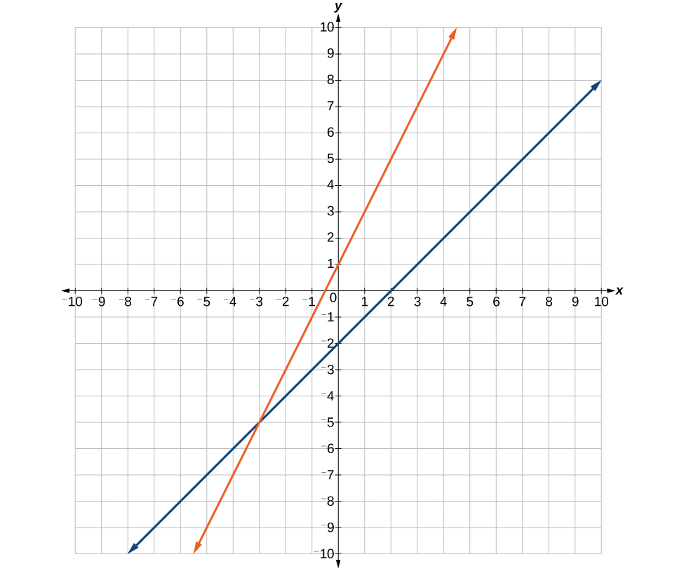
41. Where the blue line is above the orange line; always. All real numbers.
[latex]\left(-\infty ,-\infty \right)[/latex]
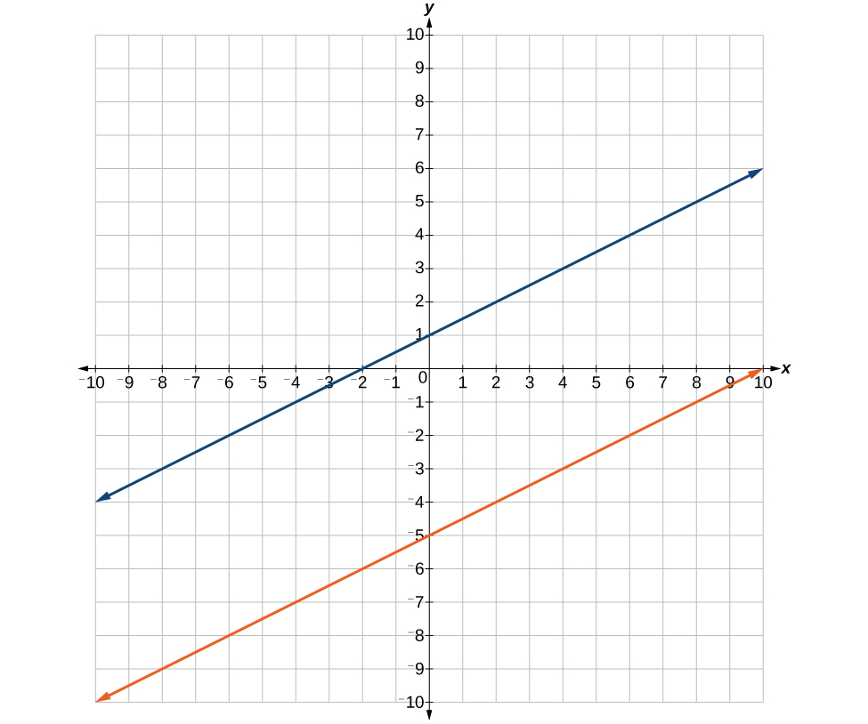
43. [latex]\left(-1,3\right)[/latex]
45. [latex]\left(-\infty ,4\right)[/latex]
47. [latex]\{x|x<6\}[/latex]
49. [latex]\{x|-3\le x<5\}[/latex]
51. [latex]\left(-2,1\right][/latex]
53. [latex]\left(-\infty ,4\right][/latex]
55. Where the blue is below the orange; always. All real numbers. [latex]\left(-\infty ,+\infty \right)[/latex].
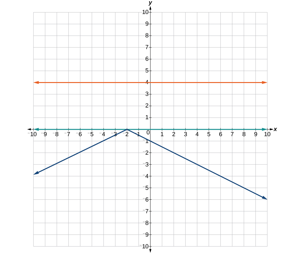
57. Where the blue is below the orange; [latex]\left(1,7\right)[/latex].
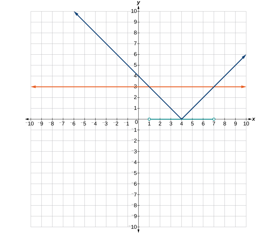
59. [latex]x=2,\frac{-4}{5}[/latex]
61. [latex]\left(-7,5\right][/latex]
63. [latex]\begin{array}{l}80\le T\le 120\\ 1,600\le 20T\le 2,400\end{array}[/latex]
[latex]\left[1,600, 2,400\right][/latex]
By the end of this lesson, you will be able to:
A jetliner changes altitude as its distance from the starting point of a flight increases. The weight of a growing child increases with time. In each case, one quantity depends on another. There is a relationship between the two quantities that we can describe, analyze, and use to make predictions. In this section, we will analyze such relationships.
A relation is a set of ordered pairs. The set of the first components of each ordered pair is called the domain and the set of the second components of each ordered pair is called the range. Consider the following set of ordered pairs. The first numbers in each pair are the first five natural numbers. The second number in each pair is twice that of the first.
The domain is [latex]\left\{1,2,3,4,5\right\}[/latex]. The range is [latex]\left\{2,4,6,8,10\right\}[/latex].
Note that each value in the domain is also known as an input value, or independent variable, and is often labeled with the lowercase letter [latex]x[/latex]. Each value in the range is also known as an output value, or dependent variable, and is often labeled lowercase letter [latex]y[/latex].
A function [latex]f[/latex] is a relation that assigns a single value in the range to each value in the domain. In other words, no x-values are repeated. For our example that relates the first five natural numbers to numbers double their values, this relation is a function because each element in the domain, [latex]\left\{1,2,3,4,5\right\}[/latex], is paired with exactly one element in the range, [latex]\left\{2,4,6,8,10\right\}[/latex].
Now let’s consider the set of ordered pairs that relates the terms “even” and “odd” to the first five natural numbers. It would appear as
Notice that each element in the domain, [latex]\left\{\text{even,}\text{odd}\right\}[/latex] is not paired with exactly one element in the range, [latex]\left\{1,2,3,4,5\right\}[/latex]. For example, the term “odd” corresponds to three values from the domain, [latex]\left\{1,3,5\right\}[/latex] and the term “even” corresponds to two values from the range, [latex]\left\{2,4\right\}[/latex]. This violates the definition of a function, so this relation is not a function.
Figure 1 compares relations that are functions and not functions.
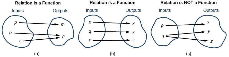
Figure 1. (a) This relationship is a function because each input is associated with a single output. Note that input [latex]q[/latex] and [latex]r[/latex] both give output [latex]n[/latex]. (b) This relationship is also a function. In this case, each input is associated with a single output. (c) This relationship is not a function because input [latex]q[/latex] is associated with two different outputs.
A function is a relation in which each possible input value leads to exactly one output value. We say “the output is a function of the input.”
The input values make up the domain, and the output values make up the range.
The coffee shop menu, shown in Figure 2 consists of items and their prices.

Figure 2

Figure 2
Each item on the menu has only one price, so the price is a function of the item.

Figure 3
Therefore, the item is a not a function of price.
In a particular math class, the overall percent grade corresponds to a grade point average. Is grade point average a function of the percent grade? Is the percent grade a function of the grade point average? The table below shows a possible rule for assigning grade points.
| Percent Grade | 0–56 | 57–61 | 62–66 | 67–71 | 72–77 | 78–86 | 87–91 | 92–100 |
|---|---|---|---|---|---|---|---|---|
| Grade Point Average | 0.0 | 1.0 | 1.5 | 2.0 | 2.5 | 3.0 | 3.5 | 4.0 |
For any percent grade earned, there is an associated grade point average, so the grade point average is a function of the percent grade. In other words, if we input the percent grade, the output is a specific grade point average.
In the grading system given, there is a range of percent grades that correspond to the same grade point average. For example, students who receive a grade point average of 3.0 could have a variety of percent grades ranging from 78 all the way to 86. Thus, percent grade is not a function of grade point average.
The table below lists the five greatest baseball players of all time in order of rank.
| Player | Rank |
|---|---|
| Babe Ruth | 1 |
| Willie Mays | 2 |
| Ty Cobb | 3 |
| Walter Johnson | 4 |
| Hank Aaron | 5 |
Once we determine that a relationship is a function, we need to display and define the functional relationships so that we can understand and use them, and sometimes also so that we can program them into computers. There are various ways of representing functions. A standard function notation is one representation that facilitates working with functions.
To represent “height is a function of age,” we start by identifying the descriptive variables [latex]h[/latex] for height and [latex]a[/latex] for age. The letters [latex]f,g[/latex], and [latex]h[/latex] are often used to represent functions just as we use [latex]x,y[/latex], and [latex]z[/latex] to represent numbers and [latex]A,B[/latex], and [latex]C[/latex] to represent sets.
Remember, we can use any letter to name the function; the notation [latex]h\left(a\right)[/latex] shows us that [latex]h[/latex] depends on [latex]a[/latex]. The value [latex]a[/latex] must be put into the function [latex]h[/latex] to get a result. The parentheses indicate that age is input into the function; they do not indicate multiplication.
We can also give an algebraic expression as the input to a function. For example [latex]f\left(a+b\right)[/latex] means “first add a and b, and the result is the input for the function f.” The operations must be performed in this order to obtain the correct result.
The notation [latex]y=f\left(x\right)[/latex] defines a function named [latex]f[/latex]. This is read as [latex]``y[/latex] is a function of [latex]x.''[/latex] The letter [latex]x[/latex] represents the input value, or independent variable. The letter [latex]y\text{,\hspace{0.17em}}[/latex] or [latex]f\left(x\right)[/latex], represents the output value, or dependent variable.
Use function notation to represent a function whose input is the name of a month and output is the number of days in that month.
The number of days in a month is a function of the name of the month, so if we name the function [latex]f[/latex], we write [latex]\text{days}=f\left(\text{month}\right)[/latex] or [latex]d=f\left(m\right)[/latex]. The name of the month is the input to a “rule” that associates a specific number (the output) with each input.

Figure 4
For example, [latex]f\left(\text{March}\right)=31[/latex], because March has 31 days. The notation [latex]d=f\left(m\right)[/latex] reminds us that the number of days, [latex]d[/latex] (the output), is dependent on the name of the month, [latex]m[/latex] (the input).
Note that the inputs to a function do not have to be numbers; function inputs can be names of people, labels of geometric objects, or any other element that determines some kind of output. However, most of the functions we will work with in this book will have numbers as inputs and outputs.
A function [latex]N=f\left(y\right)[/latex] gives the number of police officers, [latex]N[/latex], in a town in year [latex]y[/latex]. What does [latex]f\left(2005\right)=300[/latex] represent?
When we read [latex]f\left(2005\right)=300[/latex], we see that the input year is 2005. The value for the output, the number of police officers [latex]\left(N\right)[/latex], is 300. Remember, [latex]N=f\left(y\right)[/latex]. The statement [latex]f\left(2005\right)=300[/latex] tells us that in the year 2005 there were 300 police officers in the town.
Instead of a notation such as [latex]y=f\left(x\right)[/latex], could we use the same symbol for the output as for the function, such as [latex]y=y\left(x\right)[/latex], meaning “y is a function of x?”
Yes, this is often done, especially in applied subjects that use higher math, such as physics and engineering. However, in exploring math itself we like to maintain a distinction between a function such as [latex]f[/latex], which is a rule or procedure, and the output [latex]y[/latex] we get by applying [latex]f[/latex] to a particular input [latex]x[/latex]. This is why we usually use notation such as [latex]y=f\left(x\right),P=W\left(d\right)[/latex], and so on.
A common method of representing functions is in the form of a table. The table rows or columns display the corresponding input and output values. In some cases, these values represent all we know about the relationship; other times, the table provides a few select examples from a more complete relationship.
The table below lists the input number of each month (January = 1, February = 2, and so on) and the output value of the number of days in that month. This information represents all we know about the months and days for a given year (that is not a leap year). Note that, in this table, we define a days-in-a-month function [latex]f[/latex] where [latex]D=f\left(m\right)[/latex] identifies months by an integer rather than by name.
| Month number, [latex]m[/latex] (input) | 1 | 2 | 3 | 4 | 5 | 6 | 7 | 8 | 9 | 10 | 11 | 12 |
| Days in month, [latex]D[/latex] (output) | 31 | 28 | 31 | 30 | 31 | 30 | 31 | 31 | 30 | 31 | 30 | 31 |
The table below defines a function [latex]Q=g\left(n\right)[/latex]. Remember, this notation tells us that [latex]g[/latex] is the name of the function that takes the input [latex]n[/latex] and gives the output [latex]Q\text{\hspace{0.17em}.}[/latex]
| [latex]n[/latex] | 1 | 2 | 3 | 4 | 5 |
| [latex]Q[/latex] | 8 | 6 | 7 | 6 | 8 |
The table below displays the age of children in years and their corresponding heights. This table displays just some of the data available for the heights and ages of children. We can see right away that this table does not represent a function because the same input value, 5 years, has two different output values, 40 in. and 42 in.
| Age in years, [latex]\text{ }a\text{ }[/latex] (input) | 5 | 5 | 6 | 7 | 8 | 9 | 10 |
| Height in inches, [latex]\text{ }h\text{ }[/latex] (output) | 40 | 42 | 44 | 47 | 50 | 52 | 54 |
Which table, a), b), or c), represents a function (if any)?
a)
| Input | Output |
|---|---|
| 2 | 1 |
| 5 | 3 |
| 8 | 6 |
b)
| Input | Output |
|---|---|
| –3 | 5 |
| 0 | 1 |
| 4 | 5 |
c)
| Input | Output |
|---|---|
| 1 | 0 |
| 5 | 2 |
| 5 | 4 |
a) and b) define functions. In both, each input value corresponds to exactly one output value. c) does not define a function because the input value of 5 corresponds to two different output values.
When a table represents a function, corresponding input and output values can also be specified using function notation.
The function represented by a) can be represented by writing
Similarly, the statements [latex]g\left(-3\right)=5,g\left(0\right)=1,\text{and }g\left(4\right)=5[/latex] represent the function in b).
c) cannot be expressed in a similar way because it does not represent a function.
When we know an input value and want to determine the corresponding output value for a function, we evaluate the function. Evaluating will always produce one result because each input value of a function corresponds to exactly one output value.
When we know an output value and want to determine the input values that would produce that output value, we set the output equal to the function’s formula and solve for the input. Solving can produce more than one solution because different input values can produce the same output value.
When we have a function in formula form, it is usually a simple matter to evaluate the function. For example, the function [latex]f\left(x\right)=5 - 3{x}^{2}[/latex] can be evaluated by squaring the input value, multiplying by 3, and then subtracting the product from 5.
Given the function [latex]h\left(p\right)={p}^{2}+2p[/latex], evaluate [latex]h\left(4\right)[/latex].
To evaluate [latex]h\left(4\right)[/latex], we substitute the value 4 for the input variable [latex]p[/latex] in the given function.
Therefore, for an input of 4, we have an output of 24.
Evaluate [latex]f\left(x\right)={x}^{2}+3x - 4[/latex] at
Replace the [latex]x[/latex] in the function with each specified value.
and we know that
Now we combine the results and simplify.
Given the function [latex]g\left(m\right)=\sqrt{m - 4}[/latex], evaluate [latex]g\left(5\right)[/latex].
Given the function [latex]h\left(p\right)={p}^{2}+2p[/latex], solve for [latex]h\left(p\right)=3[/latex].
[latex]\begin{cases}\text{ }h\left(p\right)=3\hfill & \hfill & \hfill & \hfill \\ \text{ }{p}^{2}+2p=3\hfill & \hfill & \hfill & \text{Substitute the original function }h\left(p\right)={p}^{2}+2p.\hfill \\ \text{ }{p}^{2}+2p - 3=0\hfill & \hfill & \hfill & \text{Subtract 3 from each side}.\hfill \\ \text{ }\left(p+3\text{)(}p - 1\right)=0\hfill & \hfill & \hfill & \text{Factor}.\hfill \end{cases}[/latex]
If [latex]\left(p+3\right)\left(p - 1\right)=0[/latex], either [latex]\left(p+3\right)=0[/latex] or [latex]\left(p - 1\right)=0[/latex] (or both of them equal 0). We will set each factor equal to 0 and solve for [latex]p[/latex] in each case.
[latex]\begin{cases}\left(p+3\right)=0,\hfill & p=-3\hfill \\ \left(p - 1\right)=0,\hfill & p=1\hfill \end{cases}[/latex]
This gives us two solutions. The output [latex]h\left(p\right)=3[/latex] when the input is either [latex]p=1[/latex] or [latex]p=-3[/latex].
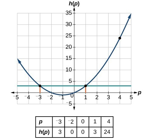
Figure 5
We can also verify by graphing as in Figure 5. The graph verifies that [latex]h\left(1\right)=h\left(-3\right)=3[/latex] and [latex]h\left(4\right)=24[/latex].
Given the function [latex]g\left(m\right)=\sqrt{m - 4}[/latex], solve [latex]g\left(m\right)=2[/latex].
Some functions are defined by mathematical rules or procedures expressed in equation form. If it is possible to express the function output with a formula involving the input quantity, then we can define a function in algebraic form. For example, the equation [latex]2n+6p=12[/latex] expresses a functional relationship between [latex]n[/latex] and [latex]p[/latex]. We can rewrite it to decide if [latex]p[/latex] is a function of [latex]n[/latex].
Express the relationship [latex]2n+6p=12[/latex] as a function [latex]p=f\left(n\right)[/latex], if possible.
To express the relationship in this form, we need to be able to write the relationship where [latex]p[/latex] is a function of [latex]n[/latex], which means writing it as p = expression involving n.
[latex]\begin{cases}2n+6p=12\hfill & \hfill \\ 6p=12 - 2n\hfill & \begin{cases}& & \end{cases}\text{Subtract }2n\text{ from both sides}.\hfill \\ p=\frac{12 - 2n}{6}\hfill & \begin{cases}& & \end{cases}\text{Divide both sides by 6 and simplify}.\hfill \\ p=\frac{12}{6}-\frac{2n}{6}\hfill & \hfill \\ p=2-\frac{1}{3}n\hfill & \hfill \end{cases}[/latex]
Therefore, [latex]p[/latex] as a function of [latex]n[/latex] is written as
It is important to note that not every relationship expressed by an equation can also be expressed as a function with a formula.
Does the equation [latex]{x}^{2}+{y}^{2}=1[/latex] represent a function with [latex]x[/latex] as input and [latex]y[/latex] as output? If so, express the relationship as a function [latex]y=f\left(x\right)[/latex].
First we subtract [latex]{x}^{2}[/latex] from both sides.
We now try to solve for [latex]y[/latex] in this equation.
We get two outputs corresponding to the same input, so this relationship cannot be represented as a single function
If [latex]x - 8{y}^{3}=0[/latex], express [latex]y[/latex] as a function of [latex]x[/latex].
Are there relationships expressed by an equation that do represent a function but which still cannot be represented by an algebraic formula?
Yes, this can happen. For example, given the equation [latex]x=y+{2}^{y}[/latex], if we want to express [latex]y[/latex] as a function of [latex]x[/latex], there is no simple algebraic formula involving only [latex]x[/latex] that equals [latex]y[/latex]. However, each [latex]x[/latex] does determine a unique value for [latex]y[/latex], and there are mathematical procedures by which [latex]y[/latex] can be found to any desired accuracy. In this case, we say that the equation gives an implicit (implied) rule for [latex]y[/latex] as a function of [latex]x[/latex], even though the formula cannot be written explicitly.
As we saw above, we can represent functions in tables. Conversely, we can use information in tables to write functions, and we can evaluate functions using the tables. For example, how well do our pets recall the fond memories we share with them? There is an urban legend that a goldfish has a memory of 3 seconds, but this is just a myth. Goldfish can remember up to 3 months, while the beta fish has a memory of up to 5 months. And while a puppy’s memory span is no longer than 30 seconds, the adult dog can remember for 5 minutes. This is meager compared to a cat, whose memory span lasts for 16 hours.
The function that relates the type of pet to the duration of its memory span is more easily visualized with the use of a table. See the table below.
| Pet | Memory span in hours |
|---|---|
| Puppy | 0.008 |
| Adult dog | 0.083 |
| Cat | 16 |
| Goldfish | 2160 |
| Beta fish | 3600 |
At times, evaluating a function in table form may be more useful than using equations. Here let us call the function [latex]P[/latex].
The domain of the function is the type of pet and the range is a real number representing the number of hours the pet’s memory span lasts. We can evaluate the function [latex]P[/latex] at the input value of “goldfish.” We would write [latex]P\left(\text{goldfish}\right)=2160[/latex]. Notice that, to evaluate the function in table form, we identify the input value and the corresponding output value from the pertinent row of the table. The tabular form for function [latex]P[/latex] seems ideally suited to this function, more so than writing it in paragraph or function form.
Using the table below,
| n | 1 | 2 | 3 | 4 | 5 |
| g(n) | 8 | 6 | 7 | 6 | 8 |
| n | 1 | 2 | 3 | 4 | 5 |
| g(n) | 8 | 6 | 7 | 6 | 8 |
When we input 2 into the function [latex]g[/latex], our output is 6. When we input 4 into the function [latex]g[/latex], our output is also 6.
Evaluating a function using a graph also requires finding the corresponding output value for a given input value, only in this case, we find the output value by looking at the graph. Solving a function equation using a graph requires finding all instances of the given output value on the graph and observing the corresponding input value(s).
Given the graph in Figure 6,
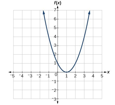
Figure 6

Figure 7

Figure 8
Figure 9
Some functions have a given output value that corresponds to two or more input values. For example, in the following stock chart the stock price was $1000 on five different dates, meaning that there were five different input values that all resulted in the same output value of $1000.
However, some functions have only one input value for each output value, as well as having only one output for each input. We call these functions one-to-one functions. As an example, consider a school that uses only letter grades and decimal equivalents, as listed in.
| Letter grade | Grade point average |
|---|---|
| A | 4.0 |
| B | 3.0 |
| C | 2.0 |
| D | 1.0 |
This grading system represents a one-to-one function, because each letter input yields one particular grade point average output and each grade point average corresponds to one input letter.
To visualize this concept, let’s look again at the two simple functions sketched in (a)and (b) of Figure 10.
Figure 10
The function in part (a) shows a relationship that is not a one-to-one function because inputs [latex]q[/latex] and [latex]r[/latex] both give output [latex]n[/latex]. The function in part (b) shows a relationship that is a one-to-one function because each input is associated with a single output.
A one-to-one function is a function in which each output value corresponds to exactly one input value.
Is the area of a circle a function of its radius? If yes, is the function one-to-one?
A circle of radius [latex]r[/latex] has a unique area measure given by [latex]A=\pi {r}^{2}[/latex], so for any input, [latex]r[/latex], there is only one output, [latex]A[/latex]. The area is a function of radius [latex]r[/latex].
If the function is one-to-one, the output value, the area, must correspond to a unique input value, the radius. Any area measure [latex]A[/latex] is given by the formula [latex]A=\pi {r}^{2}[/latex]. Because areas and radii are positive numbers, there is exactly one solution: [latex]r=\sqrt{\frac{A}{\pi }}[/latex]. So the area of a circle is a one-to-one function of the circle’s radius.
As we have seen in some examples above, we can represent a function using a graph. Graphs display a great many input-output pairs in a small space. The visual information they provide often makes relationships easier to understand. By convention, graphs are typically constructed with the input values along the horizontal axis and the output values along the vertical axis.
The most common graphs name the input value [latex]x[/latex] and the output value [latex]y[/latex], and we say [latex]y[/latex] is a function of [latex]x[/latex], or [latex]y=f\left(x\right)[/latex] when the function is named [latex]f[/latex]. The graph of the function is the set of all points [latex]\left(x,y\right)[/latex] in the plane that satisfies the equation [latex]y=f\left(x\right)[/latex]. If the function is defined for only a few input values, then the graph of the function is only a few points, where the x-coordinate of each point is an input value and the y-coordinate of each point is the corresponding output value. For example, the black dots on the graph in Figure 11 tell us that [latex]f\left(0\right)=2[/latex] and [latex]f\left(6\right)=1[/latex]. However, the set of all points [latex]\left(x,y\right)[/latex] satisfying [latex]y=f\left(x\right)[/latex] is a curve. The curve shown includes [latex]\left(0,2\right)[/latex] and [latex]\left(6,1\right)[/latex] because the curve passes through those points.
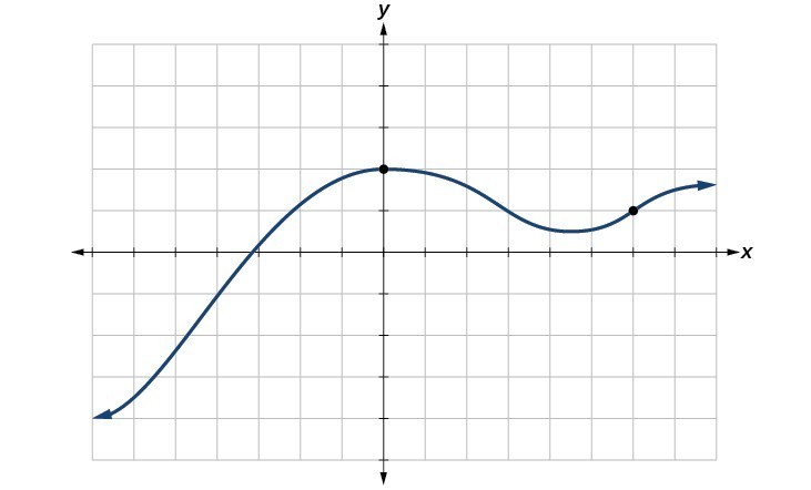
Figure 11
The vertical line test can be used to determine whether a graph represents a function. If we can draw any vertical line that intersects a graph more than once, then the graph does not define a function because a function has only one output value for each input value.
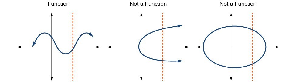
Figure 12
Which of the graphs represent(s) a function [latex]y=f\left(x\right)?[/latex]
Figure 13
If any vertical line intersects a graph more than once, the relation represented by the graph is not a function. Notice that any vertical line would pass through only one point of the two graphs shown in parts (a) and (b) of Figure 13. From this we can conclude that these two graphs represent functions. The third graph does not represent a function because, at most x-values, a vertical line would intersect the graph at more than one point.

Figure 14
Consider the functions (a), and (b)shown in the graphs in Figure 16.
Figure 16
Are either of the functions one-to-one?
The function in (a) is not one-to-one. The horizontal line shown in Figure 17 intersects the graph of the function at two points (and we can even find horizontal lines that intersect it at three points.)

Figure 17
The function in (b) is one-to-one. Any horizontal line will intersect a diagonal line at most once.
In this text, we will be exploring functions—the shapes of their graphs, their unique characteristics, their algebraic formulas, and how to solve problems with them. When learning to read, we start with the alphabet. When learning to do arithmetic, we start with numbers. When working with functions, it is similarly helpful to have a base set of building-block elements. We call these our “toolkit functions,” which form a set of basic named functions for which we know the graph, formula, and special properties. Some of these functions are programmed to individual buttons on many calculators. For these definitions we will use [latex]x[/latex] as the input variable and [latex]y=f\left(x\right)[/latex] as the output variable.
We will see these toolkit functions, combinations of toolkit functions, their graphs, and their transformations frequently throughout this book. It will be very helpful if we can recognize these toolkit functions and their features quickly by name, formula, graph, and basic table properties. The graphs and sample table values are included with each function shown below.
| Toolkit Functions | ||
|---|---|---|
| Name | Function | Graph |
| Constant | [latex]f\left(x\right)=c[/latex], where [latex]c[/latex] is a constant |  |
| Identity | [latex]f\left(x\right)=x[/latex] | 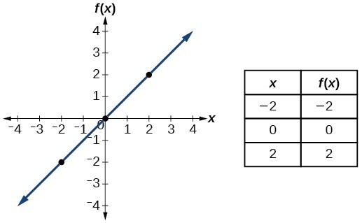 |
| Absolute value | [latex]f\left(x\right)=|x|[/latex] | 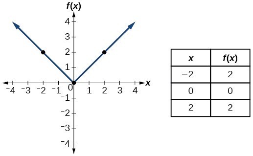 |
| Quadratic | [latex]f\left(x\right)={x}^{2}[/latex] | 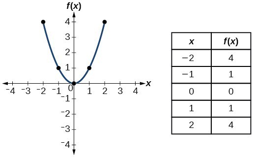 |
| Cubic | [latex]f\left(x\right)={x}^{3}[/latex] | 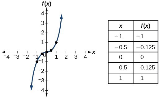 |
| Reciprocal | [latex]f\left(x\right)=\frac{1}{x}[/latex] | 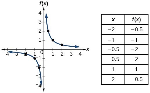 |
| Reciprocal squared | [latex]f\left(x\right)=\frac{1}{{x}^{2}}[/latex] | 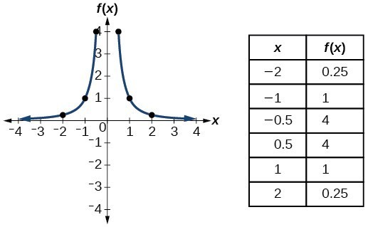 |
| Square root | [latex]f\left(x\right)=\sqrt{x}[/latex] | 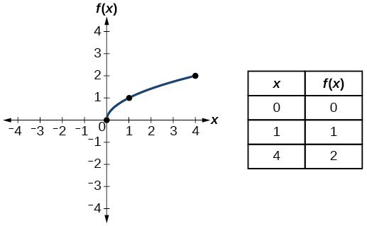 |
| Cube root | [latex]f\left(x\right)=\sqrt[3]{x}[/latex] | 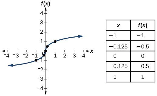 |
| Constant function | [latex]f\left(x\right)=c[/latex], where [latex]c[/latex] is a constant |
| Identity function | [latex]f\left(x\right)=x[/latex] |
| Absolute value function | [latex]f\left(x\right)=|x|[/latex] |
| Quadratic function | [latex]f\left(x\right)={x}^{2}[/latex] |
| Cubic function | [latex]f\left(x\right)={x}^{3}[/latex] |
| Reciprocal function | [latex]f\left(x\right)=\frac{1}{x}[/latex] |
| Reciprocal squared function | [latex]f\left(x\right)=\frac{1}{{x}^{2}}[/latex] |
| Square root function | [latex]f\left(x\right)=\sqrt{x}[/latex] |
| Cube root function | [latex]f\left(x\right)=\sqrt[3]{x}[/latex] |
1. What is the difference between a relation and a function?
2. What is the difference between the input and the output of a function?
3. Why does the vertical line test tell us whether the graph of a relation represents a function?
4. How can you determine if a relation is a one-to-one function?
5. Why does the horizontal line test tell us whether the graph of a function is one-to-one?
For the following exercises, determine whether the relation represents a function.
6. [latex]\left\{\left(a,b\right),\text{ }\left(c,d\right),\text{ }\left(a,c\right)\right\}[/latex]
7. [latex]\left\{\left(a,b\right),\left(b,c\right),\left(c,c\right)\right\}[/latex]
For the following exercises, determine whether the relation represents [latex]y[/latex] as a function of [latex]x[/latex].
8. [latex]5x+2y=10[/latex]
9. [latex]y={x}^{2}[/latex]
10. [latex]x={y}^{2}[/latex]
11. [latex]3{x}^{2}+y=14[/latex]
12. [latex]2x+{y}^{2}=6[/latex]
13. [latex]y=-2{x}^{2}+40x[/latex]
14. [latex]y=\frac{1}{x}[/latex]
15. [latex]x=\frac{3y+5}{7y - 1}[/latex]
16. [latex]x=\sqrt{1-{y}^{2}}[/latex]
17. [latex]y=\frac{3x+5}{7x - 1}[/latex]
18. [latex]{x}^{2}+{y}^{2}=9[/latex]
19. [latex]2xy=1[/latex]
20. [latex]x={y}^{3}[/latex]
21. [latex]y={x}^{3}[/latex]
22. [latex]y=\sqrt{1-{x}^{2}}[/latex]
23. [latex]x=\pm \sqrt{1-y}[/latex]
24. [latex]y=\pm \sqrt{1-x}[/latex]
25. [latex]{y}^{2}={x}^{2}[/latex]
26. [latex]{y}^{3}={x}^{2}[/latex]
For the following exercises, evaluate the function [latex]f[/latex] at the indicated values [latex]\text{ }f\left(-3\right),f\left(2\right),f\left(-a\right),-f\left(a\right),f\left(a+h\right)[/latex].
27. [latex]f\left(x\right)=2x - 5[/latex]
28. [latex]f\left(x\right)=-5{x}^{2}+2x - 1[/latex]
29. [latex]f\left(x\right)=\sqrt{2-x}+5[/latex]
30. [latex]f\left(x\right)=\frac{6x - 1}{5x+2}[/latex]
31. [latex]f\left(x\right)=|x - 1|-|x+1|[/latex]
32. Given the function [latex]g\left(x\right)=5-{x}^{2}[/latex], evaluate [latex]\frac{g\left(x+h\right)-g\left(x\right)}{h},h\ne 0[/latex].
33. Given the function [latex]g\left(x\right)={x}^{2}+2x[/latex], evaluate [latex]\frac{g\left(x\right)-g\left(a\right)}{x-a},x\ne a[/latex].
34. Given the function [latex]k\left(t\right)=2t - 1:[/latex]
a. Evaluate [latex]k\left(2\right)[/latex].
b. Solve [latex]k\left(t\right)=7[/latex].
35. Given the function [latex]f\left(x\right)=8 - 3x:[/latex]
a. Evaluate [latex]f\left(-2\right)[/latex].
b. Solve [latex]f\left(x\right)=-1[/latex].
36. Given the function [latex]p\left(c\right)={c}^{2}+c:[/latex]
a. Evaluate [latex]p\left(-3\right)[/latex].
b. Solve [latex]p\left(c\right)=2[/latex].
37. Given the function [latex]f\left(x\right)={x}^{2}-3x:[/latex]
a. Evaluate [latex]f\left(5\right)[/latex].
b. Solve [latex]f\left(x\right)=4[/latex].
38. Given the function [latex]f\left(x\right)=\sqrt{x+2}:[/latex]
a. Evaluate [latex]f\left(7\right)[/latex].
b. Solve [latex]f\left(x\right)=4[/latex].
39. Consider the relationship [latex]3r+2t=18[/latex].
a. Write the relationship as a function [latex]r=f\left(t\right)[/latex].
b. Evaluate [latex]f\left(-3\right)[/latex].
c. Solve [latex]f\left(t\right)=2[/latex].
For the following exercises, use the vertical line test to determine which graphs show relations that are functions.
40.

41.

42.

43.

44.

45.

46.

47.

48.

49.

50.

51.

52. Given the following graph,
a. Evaluate [latex]f\left(-1\right)[/latex].
b. Solve for [latex]f\left(x\right)=3[/latex].

53. Given the following graph,
a. Evaluate [latex]f\left(0\right)[/latex].
b. Solve for [latex]f\left(x\right)=-3[/latex].

54. Given the following graph,
a. Evaluate [latex]f\left(4\right)[/latex].
b. Solve for [latex]f\left(x\right)=1[/latex].

For the following exercises, determine if the given graph is a one-to-one function.
55.

56.

57.

58.

59.

For the following exercises, determine whether the relation represents a function.
60. [latex]\left\{\left(-1,-1\right),\left(-2,-2\right),\left(-3,-3\right)\right\}[/latex]
61. [latex]\left\{\left(3,4\right),\left(4,5\right),\left(5,6\right)\right\}[/latex]
62. [latex]\left\{\left(2,5\right),\left(7,11\right),\left(15,8\right),\left(7,9\right)\right\}[/latex]
For the following exercises, determine if the relation represented in table form represents [latex]y[/latex] as a function of [latex]x[/latex].
63.
| [latex]x[/latex] | 5 | 10 | 15 |
| [latex]y[/latex] | 3 | 8 | 14 |
64.
| [latex]x[/latex] | 5 | 10 | 15 |
| [latex]y[/latex] | 3 | 8 | 8 |
65.
| [latex]x[/latex] | 5 | 10 | 10 |
| [latex]y[/latex] | 3 | 8 | 14 |
For the following exercises, use the function [latex]f[/latex] represented in the table below.
| [latex]x[/latex] | [latex]f\left(x\right)[/latex] |
| 0 | 74 |
| 1 | 28 |
| 2 | 1 |
| 3 | 53 |
| 4 | 56 |
| 5 | 3 |
| 6 | 36 |
| 7 | 45 |
| 8 | 14 |
| 9 | 47 |
66. Evaluate [latex]f\left(3\right)[/latex].
67. Solve [latex]f\left(x\right)=1[/latex].
For the following exercises, evaluate the function [latex]f[/latex] at the values [latex]f\left(-2\right),f\left(-1\right),f\left(0\right),f\left(1\right)[/latex], and [latex]f\left(2\right)[/latex].
68. [latex]f\left(x\right)=4 - 2x[/latex]
69. [latex]f\left(x\right)=8 - 3x[/latex]
70. [latex]f\left(x\right)=8{x}^{2}-7x+3[/latex]
71. [latex]f\left(x\right)=3+\sqrt{x+3}[/latex]
72. [latex]f\left(x\right)=\frac{x - 2}{x+3}[/latex]
73. [latex]f\left(x\right)={3}^{x}[/latex]
For the following exercises, evaluate the expressions, given functions [latex]f,g[/latex], and [latex]h:[/latex]
74. [latex]3f\left(1\right)-4g\left(-2\right)[/latex]
75. [latex]f\left(\frac{7}{3}\right)-h\left(-2\right)[/latex]
For the following exercises, graph [latex]y={x}^{2}[/latex] on the given viewing window. Determine the corresponding range for each viewing window. Show each graph.
76. [latex]\left[-0.1,\text{ }0.1\right][/latex]
77. [latex]\left[-10,\text{ 10}\right][/latex]
78. [latex]\left[-100,100\right][/latex]
For the following exercises, graph [latex]y={x}^{3}[/latex] on the given viewing window. Determine the corresponding range for each viewing window. Show each graph.
79. [latex]\left[-0.1,\text{ 0}\text{.1}\right][/latex]
80. [latex]\left[-10,\text{ 10}\right][/latex]
81. [latex]\left[-100,\text{ 100}\right][/latex]
For the following exercises, graph [latex]y=\sqrt{x}[/latex] on the given viewing window. Determine the corresponding range for each viewing window. Show each graph.
82. [latex]\left[0,\text{ 0}\text{.01}\right][/latex]
83. [latex]\left[0,\text{ 100}\right][/latex]
84. [latex]\left[0,\text{ 10,000}\right][/latex]
For the following exercises, graph [latex]y=\sqrt[3]{x}[/latex] on the given viewing window. Determine the corresponding range for each viewing window. Show each graph.
85. [latex]\left[-0.001,\text{0.001}\right][/latex]
86. [latex]\left[-1000,\text{1000}\right][/latex]
87. [latex]\left[-1,000,000,\text{1,000,000}\right][/latex]
88. The amount of garbage, [latex]G[/latex], produced by a city with population [latex]p[/latex] is given by [latex]G=f\left(p\right)[/latex]. [latex]G[/latex] is measured in tons per week, and [latex]p[/latex] is measured in thousands of people.
a. The town of Tola has a population of 40,000 and produces 13 tons of garbage each week. Express this information in terms of the function [latex]f[/latex].
b. Explain the meaning of the statement [latex]f\left(5\right)=2[/latex].
89. The number of cubic yards of dirt, [latex]D[/latex], needed to cover a garden with area [latex]a[/latex] square feet is given by [latex]D=g\left(a\right)[/latex].
a. A garden with area 5000 ft2 requires 50 yd3 of dirt. Express this information in terms of the function [latex]g[/latex].
b. Explain the meaning of the statement [latex]g\left(100\right)=1[/latex].
90. Let [latex]f\left(t\right)[/latex] be the number of ducks in a lake [latex]t[/latex] years after 1990. Explain the meaning of each statement:
a. [latex]f\left(5\right)=30[/latex]
b. [latex]f\left(10\right)=40[/latex]
91. Let [latex]h\left(t\right)[/latex] be the height above ground, in feet, of a rocket [latex]t[/latex] seconds after launching. Explain the meaning of each statement:
a. [latex]h\left(1\right)=200[/latex]
b. [latex]h\left(2\right)=350[/latex]
92. Show that the function [latex]f\left(x\right)=3{\left(x - 5\right)}^{2}+7[/latex] is not one-to-one.
1. a. yes; b. yes. (Note: If two players had been tied for, say, 4th place, then the name would not have been a function of rank.)
2. [latex]g\left(5\right)=1[/latex]
3. [latex]m=8[/latex]
4. [latex]y=f\left(x\right)=\frac{\sqrt[3]{x}}{2}[/latex]
5. [latex]g\left(1\right)=8[/latex]
6. [latex]x=0[/latex] or [latex]x=2[/latex]
7. a. yes, because each bank account has a single balance at any given time; b. no, because several bank account numbers may have the same balance; c. no, because the same output may correspond to more than one input.
8. yes
1. A relation is a set of ordered pairs. A function is a special kind of relation in which no two ordered pairs have the same first coordinate.
3. When a vertical line intersects the graph of a relation more than once, that indicates that for that input there is more than one output. At any particular input value, there can be only one output if the relation is to be a function.
5. When a horizontal line intersects the graph of a function more than once, that indicates that for that output there is more than one input. A function is one-to-one if each output corresponds to only one input.
7. function
9. function
11. function
13. function
15. function
17. function
19. function
21. function
23. function
25. not a function
27. [latex]f\left(-3\right)=-11\\ f\left(2\right)=-1\\ f\left(-a\right)=-2a - 5\\-f\left(a\right)=-2a+5\\f\left(a+h\right)=2a+2h - 5\\[/latex]
29. [latex]f\left(-3\right)=\sqrt{5}+5\\ f\left(2\right)=5\\ f\left(-a\right)=\sqrt{2+a}+5\\ -f\left(a\right)=-\sqrt{2-a}-5\\f\left(a+h\right)=\\sqrt{2-a-h}+5\\[/latex]
31. [latex]f\left(-3\right)=2\\f\left(2\right)=1 - 3=-2\\f\left(-a\right)=|-a - 1|-|-a+1|\\ -f\left(a\right)=-|a - 1|+|a+1|\\\text{ }\text{ }f\left(a+h\right)=|a+h - 1|-|a+h+1|\\[/latex]
33. [latex]\frac{g\left(x\right)-g\left(a\right)}{x-a}=x+a+2,x\ne a[/latex]
35. a. [latex]f\left(-2\right)=14[/latex]; b. [latex]x=3[/latex]
37. a. [latex]f\left(5\right)=10[/latex]; b. [latex]x=-1\text{ }[/latex] or [latex]\text{ }x=4[/latex]
39. a. [latex]f\left(t\right)=6-\frac{2}{3}t[/latex]; b. [latex]f\left(-3\right)=8[/latex]; c. [latex]t=6[/latex]
41. not a function
43. function
45. function
47. function
49. function
51. function
53. a. [latex]f\left(0\right)=1[/latex]; b. [latex]f\left(x\right)=-3,x=-2\text{ }[/latex] or [latex]\text{ }x=2[/latex]
55. not a function so it is also not a one-to-one function
57. one-to-one function
59. function, but not one-to-one
61. function
63. function
65. not a function
67. [latex]f\left(x\right)=1,x=2[/latex]
69. [latex]f\left(-2\right)=14\\ f\left(-1\right)=11\\ f\left(0\right)=8\\f\left(1\right)=5\\ f\left(2\right)=2\\[/latex]
71. [latex]f\left(-2\right)=4\\\text{ }\\ f\left(-1\right)=4.414\\ f\left(0\right)=4.732\\ f\left(1\right)=4.5\\ f\left(2\right)=5.236\\[/latex]
73. [latex]f\left(-2\right)=\frac{1}{9}\\ f\left(-1\right)=\frac{1}{3}\\ f\left(0\right)=1\\ f\left(1\right)=3;\\f\left(2\right)=9\\[/latex]
75. 20
77. [latex]\left[0,\text{ 100}\right][/latex]

79.[latex]\left[-0.001,\text{ 0}\text{.001}\right][/latex]

81. [latex]\left[-1,000,000,\text{ 1,000,000}\right][/latex]

83. [latex]\left[0,\text{ 10}\right][/latex]

85. [latex]\left[-0.1,\text{0.1}\right][/latex]

87. [latex]\left[-100,\text{ 100}\right][/latex]

89. a. [latex]g\left(5000\right)=50[/latex]; b. The number of cubic yards of dirt required for a garden of 100 square feet is 1.
91. a. The height of a rocket above ground after 1 second is 200 ft. b. the height of a rocket above ground after 2 seconds is 350 ft.
By the end of this lesson, you will be able to:
If you’re in the mood for a scary movie, you may want to check out one of the five most popular horror movies of all time—I am Legend, Hannibal, The Ring, The Grudge, and The Conjuring. Figure 1 shows the amount, in dollars, each of those movies grossed when they were released as well as the ticket sales for horror movies in general by year. Notice that we can use the data to create a function of the amount each movie earned or the total ticket sales for all horror movies by year. In creating various functions using the data, we can identify different independent and dependent variables, and we can analyze the data and the functions to determine the domain and range. In this section, we will investigate methods for determining the domain and range of functions such as these.

Figure 1. Based on data compiled by www.the-numbers.com.
In Functions and Function Notation, we were introduced to the concepts of domain and range. In this section, we will practice determining domains and ranges for specific functions. Keep in mind that, in determining domains and ranges, we need to consider what is physically possible or meaningful in real-world examples, such as tickets sales and year in the horror movie example above. We also need to consider what is mathematically permitted. For example, we cannot include any input value that leads us to take an even root of a negative number if the domain and range consist of real numbers. Or in a function expressed as a formula, we cannot include any input value in the domain that would lead us to divide by 0.
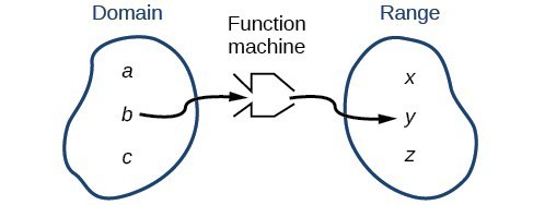
Figure 2
We can visualize the domain as a “holding area” that contains “raw materials” for a “function machine” and the range as another “holding area” for the machine’s products.
We can write the domain and range in interval notation, which uses values within brackets to describe a set of numbers. In interval notation, we use a square bracket [ when the set includes the endpoint and a parenthesis ( to indicate that the endpoint is either not included or the interval is unbounded. For example, if a person has $100 to spend, he or she would need to express the interval that is more than 0 and less than or equal to 100 and write [latex]\left(0,\text{ }100\right][/latex]. We will discuss interval notation in greater detail later.
Let’s turn our attention to finding the domain of a function whose equation is provided. Oftentimes, finding the domain of such functions involves remembering three different forms. First, if the function has no denominator or an even root, consider whether the domain could be all real numbers. Second, if there is a denominator in the function’s equation, exclude values in the domain that force the denominator to be zero. Third, if there is an even root, consider excluding values that would make the radicand negative.
Before we begin, let us review the conventions of interval notation:
The table below gives a summary of interval notation.
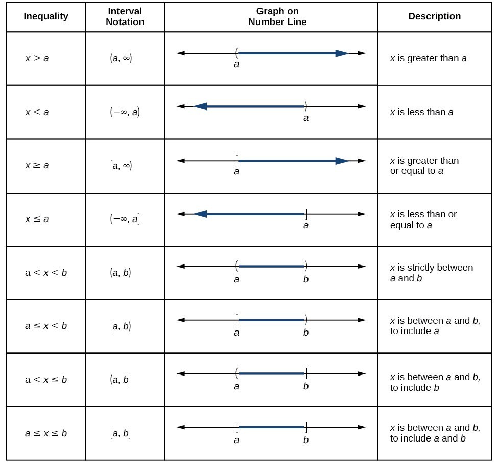
Find the domain of the following function: [latex]\left\{\left(2,\text{ }10\right),\left(3,\text{ }10\right),\left(4,\text{ }20\right),\left(5,\text{ }30\right),\left(6,\text{ }40\right)\right\}[/latex] .
First identify the input values. The input value is the first coordinate in an ordered pair. There are no restrictions, as the ordered pairs are simply listed. The domain is the set of the first coordinates of the ordered pairs.
Find the domain of the function:
[latex]\left\{\left(-5,4\right),\left(0,0\right),\left(5,-4\right),\left(10,-8\right),\left(15,-12\right)\right\}[/latex]
Find the domain of the function [latex]f\left(x\right)={x}^{2}-1[/latex].
The input value, shown by the variable [latex]x[/latex] in the equation, is squared and then the result is lowered by one. Any real number may be squared and then be lowered by one, so there are no restrictions on the domain of this function. The domain is the set of real numbers.
In interval form, the domain of [latex]f[/latex] is [latex]\left(-\infty ,\infty \right)[/latex].
Find the domain of the function [latex]f\left(x\right)=\frac{x+1}{2-x}[/latex].
When there is a denominator, we want to include only values of the input that do not force the denominator to be zero. So, we will set the denominator equal to 0 and solve for [latex]x[/latex].
Now, we will exclude 2 from the domain. The answers are all real numbers where [latex]x<2[/latex] or [latex]x>2[/latex]. We can use a symbol known as the union, [latex]\cup [/latex], to combine the two sets. In interval notation, we write the solution: [latex]\left(\mathrm{-\infty },2\right)\cup \left(2,\infty \right)[/latex].
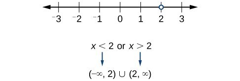
Figure 3
In interval form, the domain of [latex]f[/latex] is [latex]\left(-\infty ,2\right)\cup \left(2,\infty \right)[/latex].
Find the domain of the function: [latex]f\left(x\right)=\frac{1+4x}{2x - 1}[/latex].
Find the domain of the function [latex]f\left(x\right)=\sqrt{7-x}[/latex].
When there is an even root in the formula, we exclude any real numbers that result in a negative number in the radicand.
Set the radicand greater than or equal to zero and solve for [latex]x[/latex].
Now, we will exclude any number greater than 7 from the domain. The answers are all real numbers less than or equal to [latex]7[/latex], or [latex]\left(-\infty ,7\right][/latex].
Can there be functions in which the domain and range do not intersect at all?
Yes. For example, the function [latex]f\left(x\right)=-\frac{1}{\sqrt{x}}[/latex] has the set of all positive real numbers as its domain but the set of all negative real numbers as its range. As a more extreme example, a function’s inputs and outputs can be completely different categories (for example, names of weekdays as inputs and numbers as outputs, as on an attendance chart), in such cases the domain and range have no elements in common.
In the previous examples, we used inequalities and lists to describe the domain of functions. We can also use inequalities, or other statements that might define sets of values or data, to describe the behavior of the variable in set-builder notation. For example, [latex]\left\{x|10\le x<30\right\}[/latex] describes the behavior of [latex]x[/latex] in set-builder notation. The braces { } are read as “the set of,” and the vertical bar | is read as “such that,” so we would read [latex]\left\{x|10\le x<30\right\}[/latex] as “the set of x-values such that 10 is less than or equal to [latex]x[/latex], and [latex]x[/latex] is less than 30.”
The table below compares inequality notation, set-builder notation, and interval notation.
| Inequality Notation | Set-builder Notation | Interval Notation | |
|---|---|---|---|
 | 5 < h ≤ 10 | { h | 5 < h ≤ 10} | (5, 10] |
 | 5 ≤ h < 10 | { h | 5 ≤ h < 10} | [5, 10] |
 | 5 < h < 10 | { h | 5 < 10 } | (5, 10) |
 | h < 10 | { h | h < 10 } | ( −∞, 10) |
 | h ≥ 10 | { h | h ≥ 10 } | [10, ∞ ) |
 | All real numbers | ℝ | ( −∞, ∞ ) |
To combine two intervals using inequality notation or set-builder notation, we use the word “or.” As we saw in earlier examples, we use the union symbol, [latex]\cup [/latex], to combine two unconnected intervals. For example, the union of the sets [latex]\left\{2,3,5\right\}[/latex] and [latex]\left\{4,6\right\}[/latex] is the set [latex]\left\{2,3,4,5,6\right\}[/latex]. It is the set of all elements that belong to one or the other (or both) of the original two sets. For sets with a finite number of elements like these, the elements do not have to be listed in ascending order of numerical value. If the original two sets have some elements in common, those elements should be listed only once in the union set. For sets of real numbers on intervals, another example of a union is
This video describes how to use interval notation to describe a set.
This video describes how to use Set-Builder notation to describe a set.
Set-builder notation is a method of specifying a set of elements that satisfy a certain condition. It takes the form [latex]\left\{x|\text{statement about }x\right\}[/latex] which is read as, “the set of all [latex]x[/latex] such that the statement about [latex]x[/latex] is true.” For example,
[latex]\left\{x|4<x\le 12\right\}[/latex]
Interval notation is a way of describing sets that include all real numbers between a lower limit that may or may not be included and an upper limit that may or may not be included. The endpoint values are listed between brackets or parentheses. A square bracket indicates inclusion in the set, and a parenthesis indicates exclusion from the set. For example,
[latex]\left(4,12\right][/latex]
Describe the intervals of values shown in Figure 4 using inequality notation, set-builder notation, and interval notation.
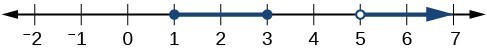
Figure 4
To describe the values, [latex]x[/latex], included in the intervals shown, we would say, ” [latex]x[/latex] is a real number greater than or equal to 1 and less than or equal to 3, or a real number greater than 5.”
| Inequality | [latex]1\le x\le 3\text{or}x>5[/latex] |
| Set-builder notation | [latex]\left\{x|1\le x\le 3\text{or}x>5\right\}[/latex] |
| Interval notation | [latex]\left[1,3\right]\cup \left(5,\infty \right)[/latex] |
Remember that, when writing or reading interval notation, using a square bracket means the boundary is included in the set. Using a parenthesis means the boundary is not included in the set.
Given Figure 5, specify the graphed set in

Figure 5
Another way to identify the domain and range of functions is by using graphs. Because the domain refers to the set of possible input values, the domain of a graph consists of all the input values shown on the x-axis. The range is the set of possible output values, which are shown on the y-axis. Keep in mind that if the graph continues beyond the portion of the graph we can see, the domain and range may be greater than the visible values. See Figure 6.
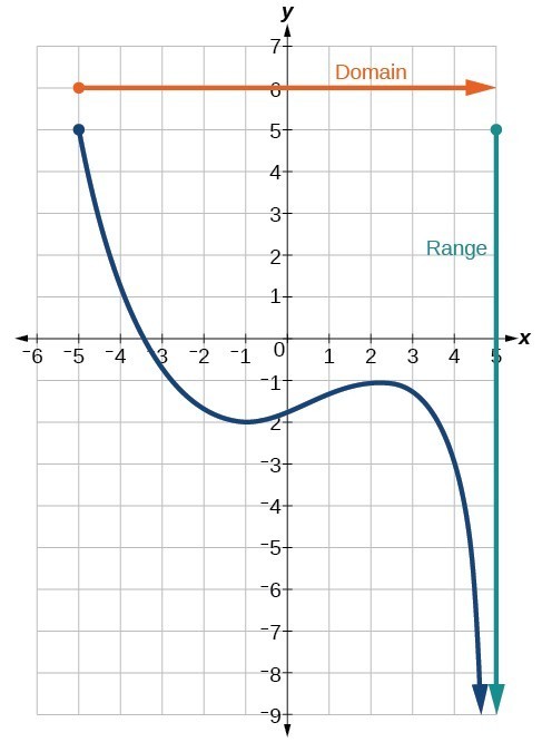
Figure 6
We can observe that the graph extends horizontally from [latex]-5[/latex] to the right without bound, so the domain is [latex]\left[-5,\infty \right)[/latex]. The vertical extent of the graph is all range values [latex]5[/latex] and below, so the range is [latex]\left(\mathrm{-\infty },5\right][/latex]. Note that the domain and range are always written from smaller to larger values, or from left to right for domain, and from the bottom of the graph to the top of the graph for range.
Find the domain and range of the function [latex]f[/latex] whose graph is shown in Figure 7.
![Graph of a function from (-3, 1].](https://s3-us-west-2.amazonaws.com/courses-images-archive-read-only/wp-content/uploads/sites/924/2015/11/25200624/CNX_Precalc_Figure_01_02_0072.jpg)
Figure 7
We can observe that the horizontal extent of the graph is –3 to 1, so the domain of [latex]f[/latex] is [latex]\left(-3,1\right][/latex].

Figure 8
The vertical extent of the graph is 0 to –4, so the range is [latex]\left[-4,0\right)[/latex].
Find the domain and range of the function [latex]f[/latex] whose graph is shown in Figure 9.
Figure 9. (credit: modification of work by the U.S. Energy Information Administration)
The input quantity along the horizontal axis is “years,” which we represent with the variable [latex]t[/latex] for time. The output quantity is “thousands of barrels of oil per day,” which we represent with the variable [latex]b[/latex] for barrels. The graph may continue to the left and right beyond what is viewed, but based on the portion of the graph that is visible, we can determine the domain as [latex]1973\le t\le 2008[/latex] and the range as approximately [latex]180\le b\le 2010[/latex].
In interval notation, the domain is [1973, 2008], and the range is about [180, 2010]. For the domain and the range, we approximate the smallest and largest values since they do not fall exactly on the grid lines.
Given the graph in Figure 10, identify the domain and range using interval notation.
Figure 10
Can a function’s domain and range be the same?
Yes. For example, the domain and range of the cube root function are both the set of all real numbers.
We will now return to our set of toolkit functions to determine the domain and range of each.
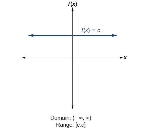
11
Figure 11. For the constant function [latex]f\left(x\right)=c[/latex], the domain consists of all real numbers; there are no restrictions on the input. The only output value is the constant [latex]c[/latex], so the range is the set [latex]\left\{c\right\}[/latex] that contains this single element. In interval notation, this is written as [latex]\left[c,c\right][/latex], the interval that both begins and ends with [latex]c[/latex].
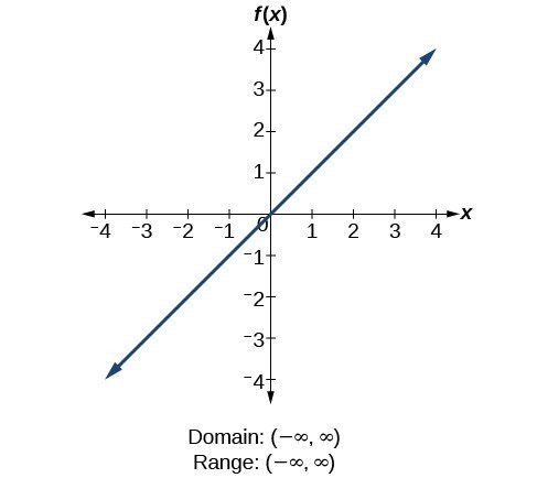
12
Figure 12. For the identity function [latex]f\left(x\right)=x[/latex], there is no restriction on [latex]x[/latex]. Both the domain and range are the set of all real numbers.
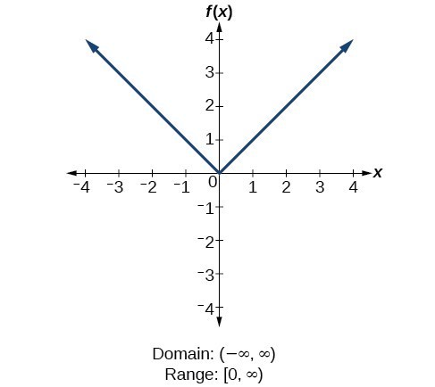
13
Figure 13. For the absolute value function [latex]f\left(x\right)=|x|[/latex], there is no restriction on [latex]x[/latex]. However, because absolute value is defined as a distance from 0, the output can only be greater than or equal to 0.
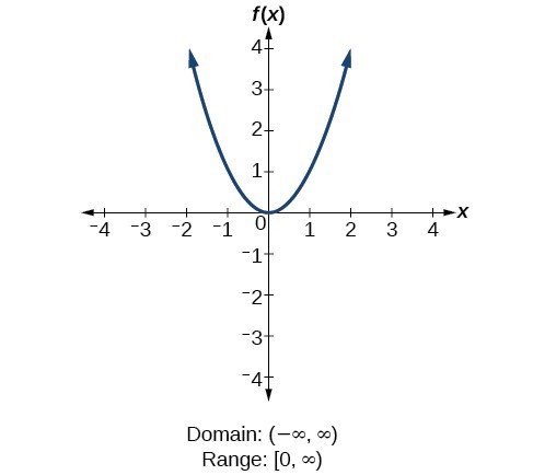
14
Figure 14. For the quadratic function [latex]f\left(x\right)={x}^{2}[/latex], the domain is all real numbers since the horizontal extent of the graph is the whole real number line. Because the graph does not include any negative values for the range, the range is only nonnegative real numbers.
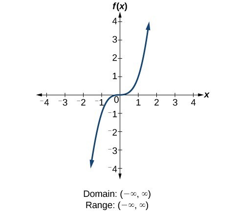
15
Figure 15. For the cubic function [latex]f\left(x\right)={x}^{3}[/latex], the domain is all real numbers because the horizontal extent of the graph is the whole real number line. The same applies to the vertical extent of the graph, so the domain and range include all real numbers.
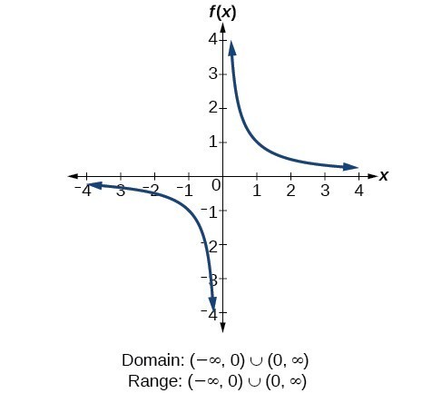
16
Figure 16. For the reciprocal function [latex]f\left(x\right)=\frac{1}{x}[/latex], we cannot divide by 0, so we must exclude 0 from the domain. Further, 1 divided by any value can never be 0, so the range also will not include 0. In set-builder notation, we could also write [latex]\left\{x|\text{ }x\ne 0\right\}[/latex], the set of all real numbers that are not zero.
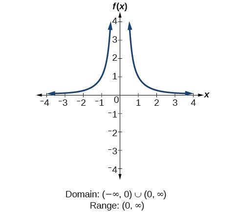
17
Figure 17. For the reciprocal squared function [latex]f\left(x\right)=\frac{1}{{x}^{2}}[/latex], we cannot divide by [latex]0[/latex], so we must exclude [latex]0[/latex] from the domain. There is also no [latex]x[/latex] that can give an output of 0, so 0 is excluded from the range as well. Note that the output of this function is always positive due to the square in the denominator, so the range includes only positive numbers.
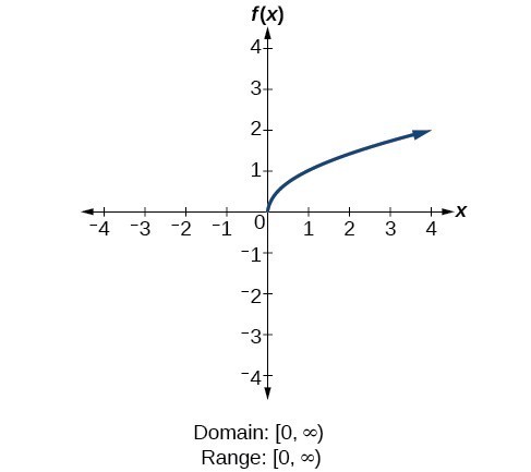
18
Figure 18. For the square root function [latex]f\left(x\right)=\sqrt[]{x}[/latex], we cannot take the square root of a negative real number, so the domain must be 0 or greater. The range also excludes negative numbers because the square root of a positive number [latex]x[/latex] is defined to be positive, even though the square of the negative number [latex]-\sqrt{x}[/latex] also gives us [latex]x[/latex].
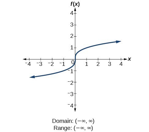
19
Figure 19. For the cube root function [latex]f\left(x\right)=\sqrt[3]{x}[/latex], the domain and range include all real numbers. Note that there is no problem taking a cube root, or any odd-integer root, of a negative number, and the resulting output is negative (it is an odd function).
Find the domain and range of [latex]f\left(x\right)=2{x}^{3}-x[/latex].
There are no restrictions on the domain, as any real number may be cubed and then subtracted from the result.
The domain is [latex]\left(-\infty ,\infty \right)[/latex] and the range is also [latex]\left(-\infty ,\infty \right)[/latex].
Find the domain and range of [latex]f\left(x\right)=\frac{2}{x+1}[/latex].
We cannot evaluate the function at [latex]-1[/latex] because division by zero is undefined. The domain is [latex]\left(-\infty ,-1\right)\cup \left(-1,\infty \right)[/latex]. Because the function is never zero, we exclude 0 from the range. The range is [latex]\left(-\infty ,0\right)\cup \left(0,\infty \right)[/latex].
Find the domain and range of [latex]f\left(x\right)=2\sqrt{x+4}[/latex].
We cannot take the square root of a negative number, so the value inside the radical must be nonnegative.
The domain of [latex]f\left(x\right)[/latex] is [latex]\left[-4,\infty \right)[/latex].
We then find the range. We know that [latex]f\left(-4\right)=0[/latex], and the function value increases as [latex]x[/latex] increases without any upper limit. We conclude that the range of [latex]f[/latex] is [latex]\left[0,\infty \right)[/latex].
Figure 20 represents the function [latex]f[/latex].

Figure 20
Sometimes, we come across a function that requires more than one formula in order to obtain the given output. For example, in the toolkit functions, we introduced the absolute value function [latex]f\left(x\right)=|x|[/latex]. With a domain of all real numbers and a range of values greater than or equal to 0, absolute value can be defined as the magnitude, or modulus, of a real number value regardless of sign. It is the distance from 0 on the number line. All of these definitions require the output to be greater than or equal to 0.
If we input 0, or a positive value, the output is the same as the input.
If we input a negative value, the output is the opposite of the input.
Because this requires two different processes or pieces, the absolute value function is an example of a piecewise function. A piecewise function is a function in which more than one formula is used to define the output over different pieces of the domain.
We use piecewise functions to describe situations in which a rule or relationship changes as the input value crosses certain “boundaries.” For example, we often encounter situations in business for which the cost per piece of a certain item is discounted once the number ordered exceeds a certain value. Tax brackets are another real-world example of piecewise functions. For example, consider a simple tax system in which incomes up to $10,000 are taxed at 10%, and any additional income is taxed at 20%. The tax on a total income, S, would be 0.1S if [latex]{S}\le\[/latex] $10,000 and 1000 + 0.2 (S – $10,000), if S> $10,000.
A piecewise function is a function in which more than one formula is used to define the output. Each formula has its own domain, and the domain of the function is the union of all these smaller domains. We notate this idea like this:
[latex] f\left(x\right)=\begin{cases}\text{formula 1 if x is in domain 1}\\ \text{formula 2 if x is in domain 2}\\ \text{formula 3 if x is in domain 3}\end{cases} [/latex]
In piecewise notation, the absolute value function is
A museum charges $5 per person for a guided tour with a group of 1 to 9 people or a fixed $50 fee for a group of 10 or more people. Write a function relating the number of people, [latex]n[/latex], to the cost, [latex]C[/latex].
Two different formulas will be needed. For n-values under 10, C=5n. For values of n that are 10 or greater, C=50.
C(n)=[latex]\begin{cases}{5n}\text{ if }{0}<{n}<{10}\\ 50\text{ if }{n}\ge 10\end{cases}[/latex]
The function is represented in Figure 21. The graph is a diagonal line from [latex]n=0[/latex] to [latex]n=10[/latex] and a constant after that. In this example, the two formulas agree at the meeting point where [latex]n=10[/latex], but not all piecewise functions have this property.
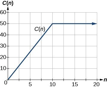
Figure 21
A cell phone company uses the function below to determine the cost, [latex]C[/latex], in dollars for [latex]g[/latex] gigabytes of data transfer.
Find the cost of using 1.5 gigabytes of data and the cost of using 4 gigabytes of data.
To find the cost of using 1.5 gigabytes of data, C(1.5), we first look to see which part of the domain our input falls in. Because 1.5 is less than 2, we use the first formula.
C(1.5) = $25
To find the cost of using 4 gigabytes of data, C(4), we see that our input of 4 is greater than 2, so we use the second formula.
The function is represented in Figure 22. We can see where the function changes from a constant to a shifted and stretched identity at [latex]g=2[/latex]. We plot the graphs for the different formulas on a common set of axes, making sure each formula is applied on its proper domain.
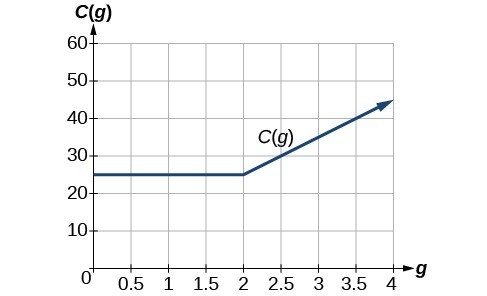
Figure 22
Sketch a graph of the function.
Each of the component functions is from our library of toolkit functions, so we know their shapes. We can imagine graphing each function and then limiting the graph to the indicated domain. At the endpoints of the domain, we draw open circles to indicate where the endpoint is not included because of a less-than or greater-than inequality; we draw a closed circle where the endpoint is included because of a less-than-or-equal-to or greater-than-or-equal-to inequality.
Below are the three components of the piecewise function graphed on separate coordinate systems.
Figure 23
Now that we have sketched each piece individually, we combine them in the same coordinate plane.
Figure 24
Note that the graph does pass the vertical line test even at [latex]x=1[/latex] and [latex]x=2[/latex] because the points [latex]\left(1,3\right)[/latex] and [latex]\left(2,2\right)[/latex] are not part of the graph of the function, though [latex]\left(1,1\right)[/latex] and [latex]\left(2,3\right)[/latex] are.
Graph the following piecewise function.
Can more than one formula from a piecewise function be applied to a value in the domain?
No. Each value corresponds to one equation in a piecewise formula.
For the following exercises, find the domain of each function using interval notation.
6. [latex]f\left(x\right)=-2x\left(x - 1\right)\left(x - 2\right)\\[/latex]
7. [latex]f\left(x\right)=5 - 2{x}^{2}\\[/latex]
8. [latex]f\left(x\right)=3\sqrt{x - 2}\\[/latex]
9. [latex]f\left(x\right)=3-\sqrt{6 - 2x}\\[/latex]
10. [latex]f\left(x\right)=\sqrt{4 - 3x}\\[/latex]
11. [latex]f\left(x\right)=\sqrt{{x}^{2}+4}\\[/latex]
12. [latex]f\left(x\right)=\sqrt[3]{1 - 2x}\\[/latex]
13. [latex]f\left(x\right)=\sqrt[3]{x - 1}\\[/latex]
14. [latex]f\left(x\right)=\frac{9}{x - 6} \\ [/latex]
15. [latex]f\left(x\right)=\frac{3x+1}{4x+2} \\[/latex]
16. [latex]f\left(x\right)=\frac{\sqrt{x+4}}{x - 4} \\[/latex]
17. [latex]f\left(x\right)=\frac{x - 3}{{x}^{2}+9x - 22} \\[/latex]
18. [latex]f\left(x\right)=\frac{1}{{x}^{2}-x - 6} \\[/latex]
19. [latex]f\left(x\right)=\frac{2{x}^{3}-250}{{x}^{2}-2x - 15} \\[/latex]
20. [latex]\frac{5}{\sqrt{x - 3}} \\[/latex]
21. [latex]\frac{2x+1}{\sqrt{5-x}} \\[/latex]
22. [latex]f\left(x\right)=\frac{\sqrt{x - 4}}{\sqrt{x - 6}} \\[/latex]
23. [latex]f\left(x\right)=\frac{\sqrt{x - 6}}{\sqrt{x - 4}} \\[/latex]
24. [latex]f\left(x\right)=\frac{x}{x} \\[/latex]
25. [latex]f\left(x\right)=\frac{{x}^{2}-9x}{{x}^{2}-81} \\[/latex]
26. Find the domain of the function [latex]f\left(x\right)=\sqrt{2{x}^{3}-50x} \\[/latex] by:
For the following exercises, write the domain and range of each function using interval notation.
27.
![Graph of a function from (2, 8].](https://s3-us-west-2.amazonaws.com/courses-images-archive-read-only/wp-content/uploads/sites/924/2015/11/25200647/CNX_Precalc_Figure_01_02_202.jpg)
Domain: ________ Range: ________
28.

29.
![Graph of a function from [-4, 4].](https://s3-us-west-2.amazonaws.com/courses-images-archive-read-only/wp-content/uploads/sites/924/2015/11/25200649/CNX_Precalc_Figure_01_02_204.jpg)
30.
![Graph of a function from [2, 6].](https://s3-us-west-2.amazonaws.com/courses-images-archive-read-only/wp-content/uploads/sites/924/2015/11/25200650/CNX_Precalc_Figure_01_02_205.jpg)
31.

32.

33.
![Graph of a function from (-infinity, 2].](https://s3-us-west-2.amazonaws.com/courses-images-archive-read-only/wp-content/uploads/sites/924/2015/11/25200654/CNX_Precalc_Figure_01_02_208.jpg)
34.

35.
![Graph of a function from [-6, -1/6]U[1/6, 6]/.](https://s3-us-west-2.amazonaws.com/courses-images-archive-read-only/wp-content/uploads/sites/924/2015/11/25200657/CNX_Precalc_Figure_01_02_210.jpg)
36.

37.

For the following exercises, sketch a graph of the piecewise function. Write the domain in interval notation.
38. [latex]f(x)=\begin{cases}{x}+{1}&\text{ if }&{ x }<{ -2 } \\{-2x - 3}&\text{ if }&{ x }\ge { -2 }\\ \end{cases} \\[/latex]
39. [latex]f\left(x\right)=\begin{cases}{2x - 1}&\text{ if }&{ x }<{ 1 }\\ {1+x }&\text{ if }&{ x }\ge{ 1 } \end{cases}\\[/latex]
40. [latex]f\left(x\right)=\begin{cases}{x+1}&\text{ if }&{ x }<{ 0 }\\ {x - 1 }&\text{ if }&{ x }>{ 0 }\end{cases}\\[/latex]
41. [latex]f\left(x\right)=\begin{cases}{3} &\text{ if }&{ x } <{ 0 }\\ \sqrt{x}&\text{ if }&{ x }\ge { 0 }\end{cases}\\[/latex]
42. [latex]f\left(x\right)=\begin{cases}{x}^{2}&\text{ if }&{ x } <{ 0 }\\ {1-x}&\text{ if }&{ x } >{ 0 }\end{cases}\\[/latex]
43. [latex]f\left(x\right)=\begin{cases}{x}^{2}&\text{ if }&{ x }<{ 0 }\\ {x+2 }&\text{ if }&{ x }\ge { 0 }\end{cases}\\[/latex]
44. [latex]f\left(x\right)=\begin{cases}x+1& \text{if}& x<1\\ {x}^{3}& \text{if}& x\ge 1\end{cases}\\[/latex]
45. [latex]f\left(x\right)=\begin{cases}|x|&\text{ if }&{ x }<{ 2 }\\ { 1 }&\text{ if }&{ x }\ge{ 2 }\end{cases}\\[/latex]
For the following exercises, given each function [latex]f[/latex], evaluate [latex]f\left(-3\right),f\left(-2\right),f\left(-1\right)[/latex], and [latex]f\left(0\right)[/latex].
46. [latex]f\left(x\right)=\begin{cases}{ x+1 }&\text{ if }&{ x }<{ -2 }\\ { -2x - 3 }&\text{ if }&{ x }\ge{ -2 }\end{cases}\\[/latex]
47. [latex]f\left(x\right)=\begin{cases}{ 1 }&\text{ if }&{ x }\le{ -3 }\\{ 0 }&\text{ if }&{ x }>{ -3 }\end{cases}\\[/latex]
48. [latex]f\left(x\right)=\begin{cases}{-2}{x}^{2}+{ 3 }&\text{ if }&{ x }\le { -1 }\\ { 5x } - { 7 } &\text{ if }&{ x } > { -1 }\end{cases}\\[/latex]
For the following exercises, given each function [latex]f[/latex], evaluate [latex]f\left(-1\right),f\left(0\right),f\left(2\right)[/latex], and [latex]f\left(4\right)[/latex].
49. [latex]f\left(x\right)=\begin{cases}{ 7x+3 }&\text{ if }&{ x }<{ 0 }\\{ 7x+6 }&\text{ if }&{ x }\ge{ 0 }\end{cases}\\[/latex]
50. [latex]f\left(x\right)=\begin{cases}{x}^{2}{ -2 }&\text{ if }&{ x }<{ 2 }\\{ 4+|x - 5|}&\text{ if }&{ x }\ge{ 2 }\end{cases}[/latex]
51. [latex]f\left(x\right)=\begin{cases}5x& \text{if}& x<0\\ 3& \text{if}& 0\le x\le 3\\ {x}^{2}& \text{if}& x>3\end{cases}[/latex]
For the following exercises, write the domain for the piecewise function in interval notation.
52. [latex]f\left(x\right)=\begin{cases}{x+1}&\text{ if }&{ x }<{ -2 }\\{ -2x - 3}&\text{ if }&{ x }\ge{ -2 }\end{cases}[/latex]
53. [latex]f\left(x\right)=\begin{cases}{x}^{2}{ -2 }&\text{ if}&{ x }<{ 1 }\\{-x}^{2}+{2}&\text{ if }&{ x }>{ 1 }\end{cases}[/latex]
54. [latex]f\left(x\right)=\begin{cases}{ 2x - 3 }&\text{ if }&{ x }<{ 0 }\\{ -3}{x}^{2}&\text{ if }&{ x }\ge{ 2 }\end{cases}[/latex]
55. Graph [latex]y=\frac{1}{{x}^{2}}[/latex] on the viewing window [latex]\left[-0.5,-0.1\right][/latex] and [latex]\left[0.1,0.5\right][/latex]. Determine the corresponding range for the viewing window. Show the graphs.
56. Graph [latex]y=\frac{1}{x}[/latex] on the viewing window [latex]\left[-0.5,-0.1\right][/latex] and [latex]\left[0.1,\text{ }0.5\right][/latex]. Determine the corresponding range for the viewing window. Show the graphs.
57. Suppose the range of a function [latex]f[/latex] is [latex]\left[-5,\text{ }8\right][/latex]. What is the range of [latex]|f\left(x\right)|?[/latex]
58. Create a function in which the range is all nonnegative real numbers.
59 .Create a function in which the domain is [latex]x>2[/latex].
60. The cost in dollars of making [latex]x[/latex] items is given by the function [latex]C\left(x\right)=10x+500[/latex].
61. The height [latex]h[/latex] of a projectile is a function of the time [latex]t[/latex] it is in the air. The height in feet for [latex]t[/latex] seconds is given by the function [latex]h\left(t\right)=-16{t}^{2}+96t[/latex]. What is the domain of the function? What does the domain mean in the context of the problem?
1. [latex]\left\{-5,0,5,10,15\right\}\\[/latex]
2. [latex]\left(-\infty ,\infty \right)\\[/latex]
3. [latex]\left(-\infty ,\frac{1}{2}\right)\cup \left(\frac{1}{2},\infty \right)\\[/latex]
4. [latex]\left[-\frac{5}{2},\infty \right)\\[/latex]
5. values that are less than or equal to –2, or values that are greater than or equal to –1 and less than 3;
[latex]\left\{x|x\le -2\text{or}-1\le x<3\right\}\\[/latex];
[latex]\left(-\infty ,-2\right]\cup \left[-1,3\right)\\[/latex]
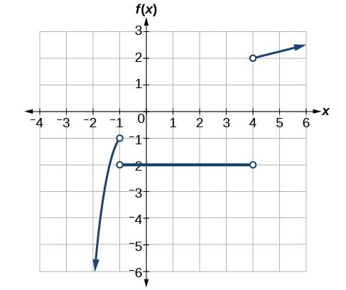
1. The domain of a function depends upon what values of the independent variable make the function undefined or imaginary.
3. There is no restriction on [latex]x[/latex] for [latex]f\left(x\right)=\sqrt[3]{x}\\[/latex] because you can take the cube root of any real number. So the domain is all real numbers, [latex]\left(-\infty ,\infty \right)\\[/latex]. When dealing with the set of real numbers, you cannot take the square root of negative numbers. So [latex]x[/latex] -values are restricted for [latex]f\left(x\right)=\sqrt[]{x}[/latex] to nonnegative numbers and the domain is [latex]\left[0,\infty \right)\\[/latex].
5. Graph each formula of the piecewise function over its corresponding domain. Use the same scale for the [latex]x[/latex] -axis and [latex]y[/latex] -axis for each graph. Indicate inclusive endpoints with a solid circle and exclusive endpoints with an open circle. Use an arrow to indicate [latex]-\infty [/latex] or [latex]\text{ }\infty \\[/latex]. Combine the graphs to find the graph of the piecewise function.
7. [latex]\left(-\infty ,\infty \right)\\[/latex]
9. [latex]\left(-\infty ,3\right]\\[/latex]
11. [latex]\left(-\infty ,\infty \right)\\[/latex]
13. [latex]\left(-\infty ,\infty \right)\\[/latex]
15. [latex]\left(-\infty ,-\frac{1}{2}\right)\cup \left(-\frac{1}{2},\infty \right)\\[/latex]
17. [latex]\left(-\infty ,-11\right)\cup \left(-11,2\right)\cup \left(2,\infty \right)\\[/latex]
19. [latex]\left(-\infty ,-3\right)\cup \left(-3,5\right)\cup \left(5,\infty \right)\\[/latex]
21. [latex]\left(-\infty ,5\right)\\[/latex]
23. [latex]\left[6,\infty \right)\\[/latex]
25. [latex]\left(-\infty ,-9\right)\cup \left(-9,9\right)\cup \left(9,\infty \right)\\[/latex]
27. Domain: [latex]\left(2,8\right][/latex] Range [latex]\left[6,8\right)\\[/latex]
29. Domain: [latex]\left[-4, 4\right][/latex] Range: [latex]\left[0, 2\right]\\[/latex]
31. Domain: [latex]\left[-5,\text{ }3\right)[/latex] Range: [latex]\left[0,2\right]\\[/latex]
33. Domain: [latex]\left(-\infty ,1\right][/latex] Range: [latex]\left[0,\infty \right)\\[/latex]
35. Domain: [latex]\left[-6,-\frac{1}{6}\right]\cup \left[\frac{1}{6},6\right]\\[/latex] Range: [latex]\left[-6,-\frac{1}{6}\right]\cup \left[\frac{1}{6},6\right]\\[/latex]
37. Domain: [latex]\left[-3,\text{ }\infty \right)\\[/latex] Range: [latex]\left[0,\infty \right)\\[/latex]
39. Domain: [latex]\left(-\infty ,\infty \right)\\[/latex]

41. Domain: [latex]\left(-\infty ,\infty \right)\\[/latex]

43. Domain: [latex]\left(-\infty ,\infty \right)\\[/latex]

45. Domain: [latex]\left(-\infty ,\infty \right)\\[/latex]

47. [latex]\begin{cases}f\left(-3\right)=1;& f\left(-2\right)=0;& f\left(-1\right)=0;& f\left(0\right)=0\end{cases}\\[/latex]
49. [latex]\begin{cases}f\left(-1\right)=-4;& f\left(0\right)=6;& f\left(2\right)=20;& f\left(4\right)=34\end{cases}\\[/latex]
51. [latex]\begin{cases}f\left(-1\right)=-5;& f\left(0\right)=3;& f\left(2\right)=3;& f\left(4\right)=16\end{cases}\\[/latex]
53. Domain: [latex]\left(-\infty ,1\right)\cup \left(1,\infty \right)\\[/latex]
55. Window: [latex]\left[-0.5,-0.1\right][/latex] Range: [latex]\left[4,\text{ }100\right]\\[/latex]
![Graph of the equation from [0.1, 0.5].](https://s3-us-west-2.amazonaws.com/courses-images-archive-read-only/wp-content/uploads/sites/924/2015/11/25200709/CNX_Precalc_Figure_01_02_222.jpg)
Window: [latex]\left[0.1,\text{ }0.5\right][/latex] Range: [latex]\left[4,\text{ }100\right][/latex]
57. [latex]\left[0,\text{ }8\right]\\[/latex]
59. Many answers. One function is [latex]f\left(x\right)=\frac{1}{\sqrt{x - 2}}\\[/latex].
61. The domain is [latex]\left[0,\text{ }6\right][/latex]; it takes 6 seconds for the projectile to leave the ground and return to the ground.
By the end of this lesson, you will be able to:
Gasoline costs have experienced some wild fluctuations over the last several decades. The table below (http://www.eia.gov/totalenergy/data/annual/showtext.cfm?t=ptb0524. Accessed 3/5/2014.) lists the average cost, in dollars, of a gallon of gasoline for the years 2005–2012. The cost of gasoline can be considered as a function of year.
| [latex]y[/latex] | 2005 | 2006 | 2007 | 2008 | 2009 | 2010 | 2011 | 2012 |
| [latex]C\left(y\right)[/latex] | 2.31 | 2.62 | 2.84 | 3.30 | 2.41 | 2.84 | 3.58 | 3.68 |
If we were interested only in how the gasoline prices changed between 2005 and 2012, we could compute that the cost per gallon had increased from $2.31 to $3.68, an increase of $1.37. While this is interesting, it might be more useful to look at how much the price changed per year. In this section, we will investigate changes such as these.
| [latex]y[/latex] | 2005 | 2006 | 2007 | 2008 | 2009 | 2010 | 2011 | 2012 |
| [latex]C\left(y\right)[/latex] | 2.31 | 2.62 | 2.84 | 3.30 | 2.41 | 2.84 | 3.58 | 3.68 |
The price change per year is a rate of change because it describes how an output quantity changes relative to the change in the input quantity. We can see that the price of gasoline in the table above did not change by the same amount each year, so the rate of change was not constant. If we use only the beginning and ending data, we would be finding the average rate of change over the specified period of time. To find the average rate of change, we divide the change in the output value by the change in the input value.
The Greek letter [latex]\Delta \\[/latex] (delta) signifies the change in a quantity; we read the ratio as “delta-y over delta-x” or “the change in [latex]y[/latex] divided by the change in [latex]x[/latex].” Occasionally we write [latex]\Delta f\\[/latex] instead of [latex]\Delta y\\[/latex], which still represents the change in the function’s output value resulting from a change to its input value. It does not mean we are changing the function into some other function.
In our example, the gasoline price increased by $1.37 from 2005 to 2012. Over 7 years, the average rate of change was
On average, the price of gas increased by about 19.6¢ each year.
Other examples of rates of change include:
A rate of change describes how an output quantity changes relative to the change in the input quantity. The units on a rate of change are “output units per input units.”
The average rate of change between two input values is the total change of the function values (output values) divided by the change in the input values.
Using the data in the table below, find the average rate of change of the price of gasoline between 2007 and 2009.
| [latex]y[/latex] | 2005 | 2006 | 2007 | 2008 | 2009 | 2010 | 2011 | 2012 |
| [latex]C\left(y\right)[/latex] | 2.31 | 2.62 | 2.84 | 3.30 | 2.41 | 2.84 | 3.58 | 3.68 |
In 2007, the price of gasoline was $2.84. In 2009, the cost was $2.41. The average rate of change is
Note that a decrease is expressed by a negative change or “negative increase.” A rate of change is negative when the output decreases as the input increases or when the output increases as the input decreases.
The following video provides another example of how to find the average rate of change between two points from a table of values.
Using the data in the table below, find the average rate of change between 2005 and 2010.
| [latex]y[/latex] | 2005 | 2006 | 2007 | 2008 | 2009 | 2010 | 2011 | 2012 |
| [latex]C\left(y\right)[/latex] | 2.31 | 2.62 | 2.84 | 3.30 | 2.41 | 2.84 | 3.58 | 3.68 |
Given the function [latex]g\left(t\right)[/latex] shown in Figure 1, find the average rate of change on the interval [latex]\left[-1,2\right][/latex].
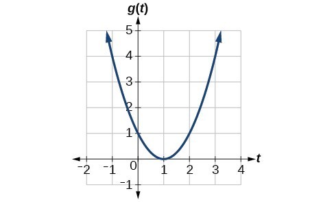
Figure 1
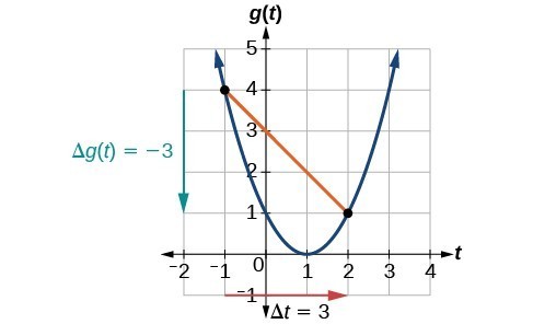
Figure 2
At [latex]t=-1[/latex], the graph shows [latex]g\left(-1\right)=4[/latex]. At [latex]t=2[/latex], the graph shows [latex]g\left(2\right)=1[/latex].
The horizontal change [latex]\Delta t=3[/latex] is shown by the red arrow, and the vertical change [latex]\Delta g\left(t\right)=-3[/latex] is shown by the turquoise arrow. The output changes by –3 while the input changes by 3, giving an average rate of change of
Note that the order we choose is very important. If, for example, we use [latex]\frac{{y}_{2}-{y}_{1}}{{x}_{1}-{x}_{2}}[/latex], we will not get the correct answer. Decide which point will be 1 and which point will be 2, and keep the coordinates fixed as [latex]\left({x}_{1},{y}_{1}\right)[/latex] and [latex]\left({x}_{2},{y}_{2}\right)[/latex].
After picking up a friend who lives 10 miles away, Anna records her distance from home over time. The values are shown in the table below. Find her average speed over the first 6 hours.
| t (hours) | 0 | 1 | 2 | 3 | 4 | 5 | 6 | 7 |
| D(t) (miles) | 10 | 55 | 90 | 153 | 214 | 240 | 282 | 300 |
Here, the average speed is the average rate of change. She traveled 282 miles in 6 hours, for an average speed of
The average speed is 47 miles per hour.
Because the speed is not constant, the average speed depends on the interval chosen. For the interval [2,3], the average speed is 63 miles per hour.
Compute the average rate of change of [latex]f\left(x\right)={x}^{2}-\frac{1}{x}[/latex] on the interval [latex]\text{[2,}\text{4].}[/latex]
We can start by computing the function values at each endpoint of the interval.
Now we compute the average rate of change.
The following video provides another example of finding the average rate of change of a function given a formula and an interval.
Find the average rate of change of [latex]f\left(x\right)=x - 2\sqrt{x}[/latex] on the interval [latex]\left[1,9\right]\\[/latex].
The electrostatic force [latex]F[/latex], measured in newtons, between two charged particles can be related to the distance between the particles [latex]d[/latex], in centimeters, by the formula [latex]F\left(d\right)=\frac{2}{{d}^{2}}[/latex]. Find the average rate of change of force if the distance between the particles is increased from 2 cm to 6 cm.
We are computing the average rate of change of [latex]F\left(d\right)=\frac{2}{{d}^{2}}[/latex] on the interval [latex]\left[2,6\right]\\[/latex].
The average rate of change is [latex]-\frac{1}{9}\\[/latex] newton per centimeter.
Find the average rate of change of [latex]g\left(t\right)={t}^{2}+3t+1[/latex] on the interval [latex]\left[0,a\right][/latex]. The answer will be an expression involving [latex]a[/latex].
We use the average rate of change formula.
This result tells us the average rate of change in terms of [latex]a[/latex] between [latex]t=0[/latex] and any other point [latex]t=a[/latex]. For example, on the interval [latex]\left[0,5\right][/latex], the average rate of change would be [latex]5+3=8[/latex].
Find the average rate of change of [latex]f\left(x\right)={x}^{2}+2x - 8[/latex] on the interval [latex]\left[5,a\right][/latex].
As part of exploring how functions change, we can identify intervals over which the function is changing in specific ways. We say that a function is increasing on an interval if the function values increase as the input values increase within that interval. Similarly, a function is decreasing on an interval if the function values decrease as the input values increase over that interval. The average rate of change of an increasing function is positive, and the average rate of change of a decreasing function is negative. Figure 3 shows examples of increasing and decreasing intervals on a function.
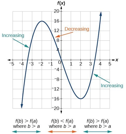
Figure 3. The function [latex]f\left(x\right)={x}^{3}-12x[/latex] is increasing on [latex]\left(-\infty \text{,}-\text{2}\right){{\cup }^{\text{ }}}^{\text{ }}\left(2,\infty \right)[/latex] and is decreasing on [latex]\left(-2\text{,}2\right)[/latex].
This video further explains how to find where a function is increasing or decreasing.
While some functions are increasing (or decreasing) over their entire domain, many others are not. A value of the input where a function changes from increasing to decreasing (as we go from left to right, that is, as the input variable increases) is called a local maximum. If a function has more than one, we say it has local maxima. Similarly, a value of the input where a function changes from decreasing to increasing as the input variable increases is called a local minimum. The plural form is “local minima.” Together, local maxima and minima are called local extrema, or local extreme values, of the function. (The singular form is “extremum.”) Often, the term local is replaced by the term relative. In this text, we will use the term local.
Clearly, a function is neither increasing nor decreasing on an interval where it is constant. A function is also neither increasing nor decreasing at extrema. Note that we have to speak of local extrema, because any given local extremum as defined here is not necessarily the highest maximum or lowest minimum in the function’s entire domain.
For the function in Figure 4, the local maximum is 16, and it occurs at [latex]x=-2[/latex]. The local minimum is [latex]-16[/latex] and it occurs at [latex]x=2[/latex].
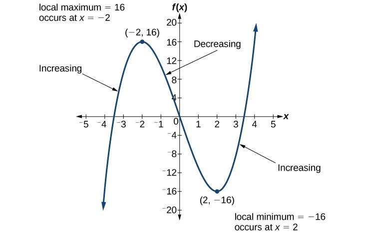
Figure 4
To locate the local maxima and minima from a graph, we need to observe the graph to determine where the graph attains its highest and lowest points, respectively, within an open interval. Like the summit of a roller coaster, the graph of a function is higher at a local maximum than at nearby points on both sides. The graph will also be lower at a local minimum than at neighboring points. Figure 5 illustrates these ideas for a local maximum.
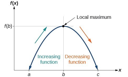
Figure 5. Definition of a local maximum.
These observations lead us to a formal definition of local extrema.
A function [latex]f[/latex] is an increasing function on an open interval if [latex]f\left(b\right)>f\left(a\right)[/latex] for any two input values [latex]a[/latex] and [latex]b[/latex] in the given interval where [latex]b>a[/latex].
A function [latex]f[/latex] is a decreasing function on an open interval if [latex]f\left(b\right)<f\left(a\right)[/latex] for any two input values [latex]a[/latex] and [latex]b[/latex] in the given interval where [latex]b>a[/latex].
A function [latex]f[/latex] has a local maximum at [latex]x=b[/latex] if there exists an interval [latex]\left(a,c\right)[/latex] with [latex]a<b<c[/latex] such that, for any [latex]x[/latex] in the interval [latex]\left(a,c\right)[/latex], [latex]f\left(x\right)\le f\left(b\right)[/latex]. Likewise, [latex]f[/latex] has a local minimum at [latex]x=b[/latex] if there exists an interval [latex]\left(a,c\right)[/latex] with [latex]a<b<c[/latex] such that, for any [latex]x[/latex] in the interval [latex]\left(a,c\right)[/latex], [latex]f\left(x\right)\ge f\left(b\right)[/latex].
Given the function [latex]p\left(t\right)[/latex] in the graph below, identify the intervals on which the function appears to be increasing.
Figure 6
We see that the function is not constant on any interval. The function is increasing where it slants upward as we move to the right and decreasing where it slants downward as we move to the right. The function appears to be increasing from [latex]t=1[/latex] to [latex]t=3[/latex] and from [latex]t=4[/latex] on.
In interval notation, we would say the function appears to be increasing on the interval (1,3) and the interval [latex]\left(4,\infty \right)[/latex].
Notice in this example that we used open intervals (intervals that do not include the endpoints), because the function is neither increasing nor decreasing at [latex]t=1[/latex] , [latex]t=3[/latex] , and [latex]t=4[/latex] . These points are the local extrema (two minima and a maximum).
Graph the function [latex]f\left(x\right)=\frac{2}{x}+\frac{x}{3}[/latex]. Then use the graph to estimate the local extrema of the function and to determine the intervals on which the function is increasing.
Using technology, we find that the graph of the function looks like that in Figure 7. It appears there is a low point, or local minimum, between [latex]x=2[/latex] and [latex]x=3[/latex], and a mirror-image high point, or local maximum, somewhere between [latex]x=-3[/latex] and [latex]x=-2[/latex].
Figure 7
Most graphing calculators and graphing utilities can estimate the location of maxima and minima. Figure 7 provides screen images from two different technologies, showing the estimate for the local maximum and minimum.
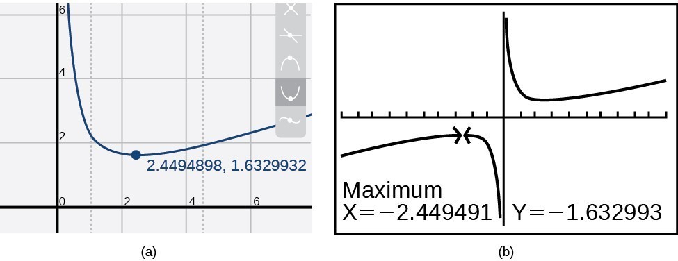
Figure 8
Based on these estimates, the function is increasing on the interval [latex]\left(-\infty ,-{2.449}\right)\\[/latex]
and [latex]\left(2.449\text{,}\infty \right)\\[/latex]. Notice that, while we expect the extrema to be symmetric, the two different technologies agree only up to four decimals due to the differing approximation algorithms used by each. (The exact location of the extrema is at [latex]\pm \sqrt{6}[/latex], but determining this requires calculus.)
Graph the function [latex]f\left(x\right)={x}^{3}-6{x}^{2}-15x+20\\[/latex] to estimate the local extrema of the function. Use these to determine the intervals on which the function is increasing and decreasing.
For the function [latex]f[/latex] whose graph is shown in Figure 9, find all local maxima and minima.
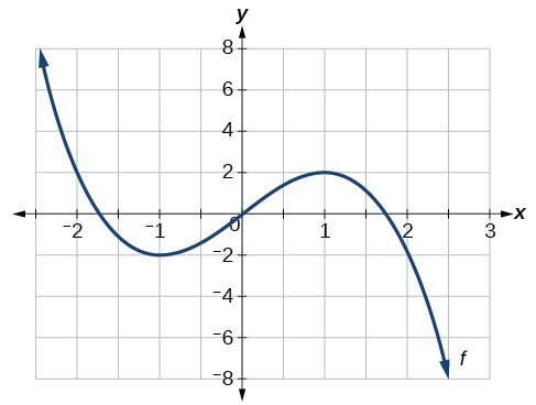
Figure 9
Observe the graph of [latex]f[/latex]. The graph attains a local maximum at [latex]x=1[/latex] because it is the highest point in an open interval around [latex]x=1[/latex]. The local maximum is the [latex]y[/latex] -coordinate at [latex]x=1[/latex], which is [latex]2[/latex].
The graph attains a local minimum at [latex]\text{ }x=-1\text{ }[/latex] because it is the lowest point in an open interval around [latex]x=-1[/latex]. The local minimum is the y-coordinate at [latex]x=-1[/latex], which is [latex]-2[/latex].
We will now return to our toolkit functions and discuss their graphical behavior in the table below.
| Function | Increasing/Decreasing | Example |
|---|---|---|
Constant Function [latex]f\left(x\right)={c}[/latex] | Neither increasing nor decreasing |  |
Identity Function [latex]f\left(x\right)={x}[/latex] | Increasing |  |
Quadratic Function [latex]f\left(x\right)={x}^{2}[/latex] | Increasing on [latex]\left(0,\infty\right)[/latex] Decreasing on [latex]\left(-\infty,0\right)[/latex] Minimum at [latex]x=0[/latex] |  |
Cubic Function [latex]f\left(x\right)={x}^{3}[/latex] | Increasing |  |
Reciprocal [latex]f\left(x\right)=\frac{1}{x}[/latex] | Decreasing [latex]\left(-\infty,0\right)\cup\left(0,\infty\right)[/latex] |  |
Reciprocal Squared [latex]f\left(x\right)=\frac{1}{{x}^{2}}[/latex] | Increasing on [latex]\left(-\infty,0\right)[/latex] Decreasing on [latex]\left(0,\infty\right)[/latex] |  |
Cube Root [latex]f\left(x\right)=\sqrt[3]{x}[/latex]
| Increasing |  |
Square Root [latex]f\left(x\right)=\sqrt{x}[/latex] | Increasing on [latex]\left(0,\infty\right)[/latex] |  |
Absolute Value [latex]f\left(x\right)=|x|[/latex] | Increasing on [latex]\left(0,\infty\right)[/latex] Decreasing on [latex]\left(-\infty,0\right)[/latex] |  |
There is a difference between locating the highest and lowest points on a graph in a region around an open interval (locally) and locating the highest and lowest points on the graph for the entire domain. The [latex]y\text{-}[/latex] coordinates (output) at the highest and lowest points are called the absolute maximum and absolute minimum, respectively.
To locate absolute maxima and minima from a graph, we need to observe the graph to determine where the graph attains it highest and lowest points on the domain of the function. See Figure 10.
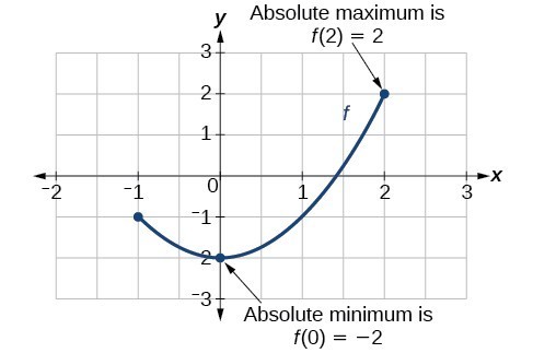
Figure 10
Not every function has an absolute maximum or minimum value. The toolkit function [latex]f\left(x\right)={x}^{3}[/latex] is one such function.
The absolute maximum of [latex]f[/latex] at [latex]x=c[/latex] is [latex]f\left(c\right)[/latex] where [latex]f\left(c\right)\ge f\left(x\right)[/latex] for all [latex]x[/latex] in the domain of [latex]f[/latex].
The absolute minimum of [latex]f[/latex] at [latex]x=d[/latex] is [latex]f\left(d\right)[/latex] where [latex]f\left(d\right)\le f\left(x\right)[/latex] for all [latex]x[/latex] in the domain of [latex]f[/latex].
For the function [latex]f[/latex] shown in Figure 11, find all absolute maxima and minima.
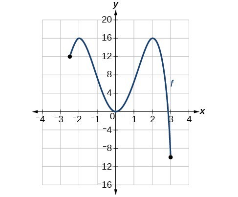
Figure 11
Observe the graph of [latex]f[/latex]. The graph attains an absolute maximum in two locations, [latex]x=-2[/latex] and [latex]x=2[/latex], because at these locations, the graph attains its highest point on the domain of the function. The absolute maximum is the y-coordinate at [latex]x=-2[/latex] and [latex]x=2[/latex], which is [latex]16[/latex].
The graph attains an absolute minimum at [latex]x=3[/latex], because it is the lowest point on the domain of the function’s graph. The absolute minimum is the y-coordinate at [latex]x=3[/latex], which is [latex]-10[/latex].
| Average rate of change | [latex]\frac{\Delta y}{\Delta x}=\frac{f\left({x}_{2}\right)-f\left({x}_{1}\right)}{{x}_{2}-{x}_{1}}[/latex] |
1. Can the average rate of change of a function be constant?
2. If a function [latex]f[/latex] is increasing on [latex]\left(a,b\right)[/latex] and decreasing on [latex]\left(b,c\right)[/latex], then what can be said about the local extremum of [latex]f[/latex] on [latex]\left(a,c\right)?[/latex]
3. How are the absolute maximum and minimum similar to and different from the local extrema?
4. How does the graph of the absolute value function compare to the graph of the quadratic function, [latex]y={x}^{2}[/latex], in terms of increasing and decreasing intervals?
For exercises 5–15, find the average rate of change of each function on the interval specified for real numbers [latex]b[/latex] or [latex]h[/latex].
5. [latex]f\left(x\right)=4{x}^{2}-7[/latex] on [latex]\left[1,\text{ }b\right]\\[/latex]
6. [latex]g\left(x\right)=2{x}^{2}-9[/latex] on [latex]\left[4,\text{ }b\right]\\[/latex]
7. [latex]p\left(x\right)=3x+4[/latex] on [latex]\left[2,\text{ }2+h\right]\\[/latex]
8. [latex]k\left(x\right)=4x - 2[/latex] on [latex]\left[3,\text{ }3+h\right]\\[/latex]
9. [latex]f\left(x\right)=2{x}^{2}+1[/latex] on [latex]\left[x,x+h\right]\\[/latex]
10. [latex]g\left(x\right)=3{x}^{2}-2[/latex] on [latex]\left[x,x+h\right]\\[/latex]
11. [latex]a\left(t\right)=\frac{1}{t+4}[/latex] on [latex]\left[9,9+h\right]\\[/latex]
12. [latex]b\left(x\right)=\frac{1}{x+3}[/latex] on [latex]\left[1,1+h\right]\\[/latex]
13. [latex]j\left(x\right)=3{x}^{3}[/latex] on [latex]\left[1,1+h\right]\\[/latex]
14. [latex]r\left(t\right)=4{t}^{3}[/latex] on [latex]\left[2,2+h\right]\\[/latex]
15. [latex]\frac{f\left(x+h\right)-f\left(x\right)}{h}\\[/latex] given [latex]f\left(x\right)=2{x}^{2}-3x\\[/latex] on [latex]\left[x,x+h\right]\\[/latex]
For exercises 16–17, consider the graph of [latex]f[/latex].
16. Estimate the average rate of change from [latex]x=1[/latex] to [latex]x=4[/latex].
17. Estimate the average rate of change from [latex]x=2[/latex] to [latex]x=5[/latex].
For exercises 18–21, use the graph of each function to estimate the intervals on which the function is increasing or decreasing.
18.
19.
20.
21.
For exercises 22–23, consider the graph shown below.
22. Estimate the intervals where the function is increasing or decreasing.
23. Estimate the point(s) at which the graph of [latex]f[/latex] has a local maximum or a local minimum.
For exercises 24–25, consider the graph below.
24. If the complete graph of the function is shown, estimate the intervals where the function is increasing or decreasing.
25. If the complete graph of the function is shown, estimate the absolute maximum and absolute minimum.
26. The table below gives the annual sales (in millions of dollars) of a product from 1998 to 2006. What was the average rate of change of annual sales (a) between 2001 and 2002, and (b) between 2001 and 2004?
| Year | Sales (millions of dollars) |
| 1998 | 201 |
| 1999 | 219 |
| 2000 | 233 |
| 2001 | 243 |
| 2002 | 249 |
| 2003 | 251 |
| 2004 | 249 |
| 2005 | 243 |
| 2006 | 233 |
27. The table below gives the population of a town (in thousands) from 2000 to 2008. What was the average rate of change of population (a) between 2002 and 2004, and (b) between 2002 and 2006?
| Year | Population (thousands) |
| 2000 | 87 |
| 2001 | 84 |
| 2002 | 83 |
| 2003 | 80 |
| 2004 | 77 |
| 2005 | 76 |
| 2006 | 78 |
| 2007 | 81 |
| 2008 | 85 |
For the following exercises, find the average rate of change of each function on the interval specified.
28. [latex]f\left(x\right)={x}^{2}[/latex] on [latex]\left[1,\text{ }5\right]\\[/latex]
29. [latex]h\left(x\right)=5 - 2{x}^{2}[/latex] on [latex]\left[-2,\text{4}\right]\\[/latex]
30. [latex]q\left(x\right)={x}^{3}[/latex] on [latex]\left[-4,\text{2}\right]\\[/latex]
31. [latex]g\left(x\right)=3{x}^{3}-1[/latex] on [latex]\left[-3,\text{3}\right]\\[/latex]
32. [latex]y=\frac{1}{x}[/latex] on [latex]\left[1,\text{ 3}\right]\\[/latex]
33. [latex]p\left(t\right)=\frac{\left({t}^{2}-4\right)\left(t+1\right)}{{t}^{2}+3}\\[/latex] on [latex]\left[-3,\text{1}\right]\\[/latex]
34. [latex]k\left(t\right)=6{t}^{2}+\frac{4}{{t}^{3}}\\[/latex] on [latex]\left[-1,3\right]\\[/latex]
For the following exercises, use a graphing utility to estimate the local extrema of each function and to estimate the intervals on which the function is increasing and decreasing.
35. [latex]f\left(x\right)={x}^{4}-4{x}^{3}+5\\[/latex]
36. [latex]h\left(x\right)={x}^{5}+5{x}^{4}+10{x}^{3}+10{x}^{2}-1\\[/latex]
37. [latex]g\left(t\right)=t\sqrt{t+3}\\[/latex]
38. [latex]k\left(t\right)=3{t}^{\frac{2}{3}}-t\\[/latex]
39. [latex]m\left(x\right)={x}^{4}+2{x}^{3}-12{x}^{2}-10x+4\\[/latex]
40. [latex]n\left(x\right)={x}^{4}-8{x}^{3}+18{x}^{2}-6x+2\\[/latex]
41.The graph of the function [latex]f[/latex] is shown below.
Based on the calculator screenshot, the point [latex]\left(1.333,\text{ }5.185\right)\\[/latex] is which of the following?
A) a relative (local) maximum of the function
B) the vertex of the function
C) the absolute maximum of the function
D) a zero of the function.
42. Let [latex]f\left(x\right)=\frac{1}{x}\\[/latex]. Find a number [latex]c[/latex] such that the average rate of change of the function [latex]f[/latex] on the interval [latex]\left(1,c\right)\\[/latex] is [latex]-\frac{1}{4}\\[/latex].
43. Let [latex]f\left(x\right)=\frac{1}{x}[/latex] . Find the number [latex]b[/latex] such that the average rate of change of [latex]f[/latex] on the interval [latex]\left(2,b\right)\\[/latex] is [latex]-\frac{1}{10}\\[/latex].
44. At the start of a trip, the odometer on a car read 21,395. At the end of the trip, 13.5 hours later, the odometer read 22,125. Assume the scale on the odometer is in miles. What is the average speed the car traveled during this trip?
45. A driver of a car stopped at a gas station to fill up his gas tank. He looked at his watch, and the time read exactly 3:40 p.m. At this time, he started pumping gas into the tank. At exactly 3:44, the tank was full and he noticed that he had pumped 10.7 gallons. What is the average rate of flow of the gasoline into the gas tank?
46. Near the surface of the moon, the distance that an object falls is a function of time. It is given by [latex]d\left(t\right)=2.6667{t}^{2}\\[/latex], where [latex]t[/latex] is in seconds and [latex]d\left(t\right)[/latex] is in feet. If an object is dropped from a certain height, find the average velocity of the object from [latex]t=1[/latex] to [latex]t=2[/latex].
47. The graph below illustrates the decay of a radioactive substance over [latex]t[/latex] days.
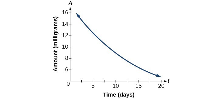
Use the graph to estimate the average decay rate from [latex]t=5[/latex] to [latex]t=15[/latex].
1. [latex]\frac{$2.84-$2.31}{5\text{ years}}=\frac{$0.53}{5\text{ years}}=$0.106[/latex] per year.
2. [latex]\frac{1}{2}\\[/latex]
3. [latex]a+7\\[/latex]
4. The local maximum appears to occur at [latex]\left(-1,28\right)[/latex], and the local minimum occurs at [latex]\left(5,-80\right)[/latex]. The function is increasing on [latex]\left(-\infty ,-1\right)\cup \left(5,\infty \right)\\[/latex] and decreasing on [latex]\left(-1,5\right)\\[/latex].

1. Yes, the average rate of change of all linear functions is constant.
3. The absolute maximum and minimum relate to the entire graph, whereas the local extrema relate only to a specific region around an open interval.
5. [latex]4\left(b+1\right)\\[/latex]
7. 3
9. [latex]4x+2h[/latex]
11. [latex]\frac{-1}{13\left(13+h\right)}\\[/latex]
13. [latex]3{h}^{2}+9h+9\\[/latex]
15. [latex]4x+2h - 3\\[/latex]
17. [latex]\frac{4}{3}\\[/latex]
19. increasing on [latex]\left(-\infty ,-2.5\right)\cup \left(1,\infty \right)\\[/latex], decreasing on [latex]\left(-2.5,\text{ }1\right)\\[/latex]
21. increasing on [latex]\left(-\infty ,1\right)\cup \left(3,4\right)\\[/latex], decreasing on [latex]\left(1,3\right)\cup \left(4,\infty \right)\\[/latex]
23. local maximum: [latex]\left(-3,\text{ }60\right)\\[/latex], local minimum: [latex]\left(3,\text{ }-60\right)\\[/latex]
25. absolute maximum at approximately [latex]\left(7,\text{ }150\right)\\[/latex], absolute minimum at approximately [latex]\left(-7.5,\text{ }-220\right)\\[/latex]
27. a. –3000; b. –1250
29. –4
31. 27
33. –0.167
35. Local minimum at [latex]\left(3,-22\right)\\[/latex], decreasing on [latex]\left(-\infty ,\text{ }3\right)\\[/latex], increasing on [latex]\left(3,\text{ }\infty \right)\\[/latex]
37. Local minimum at [latex]\left(-2,-2\right)\\[/latex], decreasing on [latex]\left(-3,-2\right)\\[/latex], increasing on [latex]\left(-2,\text{ }\infty \right)\\[/latex]
39. Local maximum at [latex]\left(-0.5,\text{ }6\right)\\[/latex], local minima at [latex]\left(-3.25,-47\right)\\[/latex] and [latex]\left(2.1,-32\right)\\[/latex], decreasing on [latex]\left(-\infty ,-3.25\right)\\[/latex] and [latex]\left(-0.5,\text{ }2.1\right)\\[/latex], increasing on [latex]\left(-3.25,\text{ }-0.5\right)\\[/latex] and [latex]\left(2.1,\text{ }\infty \right)\\[/latex]
41. A) a relative (local) maximum of the function
43. [latex]b=5[/latex]
45. 2.7 gallons per minute
47. approximately –0.6 milligrams per day
By the end of this lesson, you will be able to:
Suppose we want to calculate how much it costs to heat a house on a particular day of the year. The cost to heat a house will depend on the average daily temperature, and in turn, the average daily temperature depends on the particular day of the year. Notice how we have just defined two relationships: The cost depends on the temperature, and the temperature depends on the day.

Figure 1
Using descriptive variables, we can notate these two functions. The function [latex]C\left(T\right)[/latex] gives the cost [latex]C[/latex] of heating a house for a given average daily temperature in [latex]T[/latex] degrees Celsius. The function [latex]T\left(d\right)[/latex] gives the average daily temperature on day [latex]d[/latex] of the year. For any given day, [latex]\text{Cost}=C\left(T\left(d\right)\right)[/latex] means that the cost depends on the temperature, which in turns depends on the day of the year. Thus, we can evaluate the cost function at the temperature [latex]T\left(d\right)[/latex]. For example, we could evaluate [latex]T\left(5\right)[/latex] to determine the average daily temperature on the 5th day of the year. Then, we could evaluate the cost function at that temperature. We would write [latex]C\left(T\left(5\right)\right)[/latex].
By combining these two relationships into one function, we have performed function composition, which is the focus of this section.
Function composition is only one way to combine existing functions. Another way is to carry out the usual algebraic operations on functions, such as addition, subtraction, multiplication and division. We do this by performing the operations with the function outputs, defining the result as the output of our new function.
Suppose we need to add two columns of numbers that represent a husband and wife’s separate annual incomes over a period of years, with the result being their total household income. We want to do this for every year, adding only that year’s incomes and then collecting all the data in a new column. If [latex]w\left(y\right)[/latex] is the wife’s income and [latex]h\left(y\right)[/latex] is the husband’s income in year [latex]y[/latex], and we want [latex]T[/latex] to represent the total income, then we can define a new function.
If this holds true for every year, then we can focus on the relation between the functions without reference to a year and write
Just as for this sum of two functions, we can define difference, product, and ratio functions for any pair of functions that have the same kinds of inputs (not necessarily numbers) and also the same kinds of outputs (which do have to be numbers so that the usual operations of algebra can apply to them, and which also must have the same units or no units when we add and subtract). In this way, we can think of adding, subtracting, multiplying, and dividing functions.
For two functions [latex]f\left(x\right)[/latex] and [latex]g\left(x\right)[/latex] with real number outputs, we define new functions [latex]f+g,f-g,fg[/latex], and [latex]\frac{f}{g}[/latex] by the relations
Find and simplify the functions [latex]\left(g-f\right)\left(x\right)[/latex] and [latex]\left(\frac{g}{f}\right)\left(x\right)[/latex], given [latex]f\left(x\right)=x - 1[/latex] and [latex]g\left(x\right)={x}^{2}-1[/latex]. Are they the same function?
Begin by writing the general form, and then substitute the given functions.
No, the functions are not the same.
Note: For [latex]\left(\frac{g}{f}\right)\left(x\right)\\[/latex], the condition [latex]x\ne 1[/latex] is necessary because when [latex]x=1[/latex], the denominator is equal to 0, which makes the function undefined.
Find and simplify the functions [latex]\left(fg\right)\left(x\right)[/latex] and [latex]\left(f-g\right)\left(x\right)[/latex].
Are they the same function?
Performing algebraic operations on functions combines them into a new function, but we can also create functions by composing functions. When we wanted to compute a heating cost from a day of the year, we created a new function that takes a day as input and yields a cost as output. The process of combining functions so that the output of one function becomes the input of another is known as a composition of functions. The resulting function is known as a composite function. We represent this combination by the following notation:
[latex]\left(f\circ g\right)\left(x\right)=f\left(g\left(x\right)\right)[/latex]
We read the left-hand side as [latex]``f[/latex] composed with [latex]g[/latex] at [latex]x,''[/latex] and the right-hand side as [latex]``f[/latex] of [latex]g[/latex] of [latex]x.''[/latex] The two sides of the equation have the same mathematical meaning and are equal. The open circle symbol [latex]\circ [/latex] is called the composition operator. We use this operator mainly when we wish to emphasize the relationship between the functions themselves without referring to any particular input value. Composition is a binary operation that takes two functions and forms a new function, much as addition or multiplication takes two numbers and gives a new number. However, it is important not to confuse function composition with multiplication because, as we learned above, in most cases [latex]f\left(g\left(x\right)\right)\ne f\left(x\right)g\left(x\right)[/latex].
It is also important to understand the order of operations in evaluating a composite function. We follow the usual convention with parentheses by starting with the innermost parentheses first, and then working to the outside. In the equation above, the function [latex]g[/latex] takes the input [latex]x[/latex] first and yields an output [latex]g\left(x\right)[/latex]. Then the function [latex]f[/latex] takes [latex]g\left(x\right)[/latex] as an input and yields an output [latex]f\left(g\left(x\right)\right)[/latex].
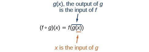
Figure 2
In general, [latex]f\circ g[/latex] and [latex]g\circ f[/latex] are different functions. In other words, in many cases [latex]f\left(g\left(x\right)\right)\ne g\left(f\left(x\right)\right)[/latex] for all [latex]x[/latex]. We will also see that sometimes two functions can be composed only in one specific order.
For example, if [latex]f\left(x\right)={x}^{2}[/latex] and [latex]g\left(x\right)=x+2[/latex], then
[latex]\begin{cases}\text{ }f\left(g\left(x\right)\right)=f\left(x+2\right)\hfill \\ \text{ }={\left(x+2\right)}^{2}\hfill \\ \text{ }={x}^{2}+4x+4\hfill \end{cases}[/latex]
but
[latex]\begin{cases}\text{ }g\left(f\left(x\right)\right)=g\left({x}^{2}\right)\hfill \\ \text{ }={x}^{2}+2\hfill \end{cases}[/latex]
These expressions are not equal for all values of [latex]x[/latex], so the two functions are not equal. It is irrelevant that the expressions happen to be equal for the single input value [latex]x=-\frac{1}{2}[/latex].
Note that the range of the inside function (the first function to be evaluated) needs to be within the domain of the outside function. Less formally, the composition has to make sense in terms of inputs and outputs.
When the output of one function is used as the input of another, we call the entire operation a composition of functions. For any input [latex]x[/latex] and functions [latex]f[/latex] and [latex]g[/latex], this action defines a composite function, which we write as [latex]f\circ g[/latex] such that
[latex]\left(f\circ g\right)\left(x\right)=f\left(g\left(x\right)\right)[/latex]
The domain of the composite function [latex]f\circ g[/latex] is all [latex]x[/latex] such that [latex]x[/latex] is in the domain of [latex]g[/latex] and [latex]g\left(x\right)[/latex] is in the domain of [latex]f[/latex].
It is important to realize that the product of functions [latex]fg[/latex] is not the same as the function composition [latex]f\left(g\left(x\right)\right)[/latex], because, in general, [latex]f\left(x\right)g\left(x\right)\ne f\left(g\left(x\right)\right)[/latex].
Using the functions provided, find [latex]f\left(g\left(x\right)\right)[/latex] and [latex]g\left(f\left(x\right)\right)[/latex]. Determine whether the composition of the functions is commutative.
[latex]f\left(x\right)=2x+1g\left(x\right)=3-x[/latex]
Let’s begin by substituting [latex]g\left(x\right)[/latex] into [latex]f\left(x\right)[/latex].[latex]\begin{cases}f\left(g\left(x\right)\right)=2\left(3-x\right)+1\hfill \\ \text{ }=6 - 2x+1\hfill \\ \text{ }=7 - 2x\hfill \end{cases}[/latex]
Now we can substitute [latex]f\left(x\right)[/latex] into [latex]g\left(x\right)[/latex].
[latex]\begin{cases}g\left(f\left(x\right)\right)=3-\left(2x+1\right)\hfill \\ \text{ }=3 - 2x - 1\hfill \\ \text{ }=-2x+2\hfill \end{cases}[/latex]
We find that [latex]g\left(f\left(x\right)\right)\ne f\left(g\left(x\right)\right)[/latex], so the operation of function composition is not commutative.
The function [latex]c\left(s\right)[/latex] gives the number of calories burned completing [latex]s[/latex] sit-ups, and [latex]s\left(t\right)[/latex] gives the number of sit-ups a person can complete in [latex]t[/latex] minutes. Interpret [latex]c\left(s\left(3\right)\right)[/latex].
The inside expression in the composition is [latex]s\left(3\right)[/latex]. Because the input to the s-function is time, [latex]t=3[/latex] represents 3 minutes, and [latex]s\left(3\right)[/latex] is the number of sit-ups completed in 3 minutes.
Using [latex]s\left(3\right)[/latex] as the input to the function [latex]c\left(s\right)[/latex] gives us the number of calories burned during the number of sit-ups that can be completed in 3 minutes, or simply the number of calories burned in 3 minutes (by doing sit-ups).
Suppose [latex]f\left(x\right)[/latex] gives miles that can be driven in [latex]x[/latex] hours and [latex]g\left(y\right)[/latex] gives the gallons of gas used in driving [latex]y[/latex] miles. Which of these expressions is meaningful: [latex]f\left(g\left(y\right)\right)[/latex] or [latex]g\left(f\left(x\right)\right)?[/latex]
The function [latex]y=f\left(x\right)[/latex] is a function whose output is the number of miles driven corresponding to the number of hours driven.
[latex]\text{number of miles }=f\left(\text{number of hours}\right)[/latex]
The function [latex]g\left(y\right)[/latex] is a function whose output is the number of gallons used corresponding to the number of miles driven. This means:
[latex]\text{number of gallons }=g\left(\text{number of miles}\right)[/latex]
The expression [latex]g\left(y\right)[/latex] takes miles as the input and a number of gallons as the output. The function [latex]f\left(x\right)[/latex] requires a number of hours as the input. Trying to input a number of gallons does not make sense. The expression [latex]f\left(g\left(y\right)\right)[/latex] is meaningless.
The expression [latex]f\left(x\right)[/latex] takes hours as input and a number of miles driven as the output. The function [latex]g\left(y\right)[/latex] requires a number of miles as the input. Using [latex]f\left(x\right)[/latex] (miles driven) as an input value for [latex]g\left(y\right)[/latex], where gallons of gas depends on miles driven, does make sense. The expression [latex]g\left(f\left(x\right)\right)[/latex] makes sense, and will yield the number of gallons of gas used, [latex]g[/latex], driving a certain number of miles, [latex]f\left(x\right)[/latex], in [latex]x[/latex] hours.
Are there any situations where [latex]f\left(g\left(y\right)\right)[/latex] and [latex]g\left(f\left(x\right)\right)[/latex] would both be meaningful or useful expressions?
Yes. For many pure mathematical functions, both compositions make sense, even though they usually produce different new functions. In real-world problems, functions whose inputs and outputs have the same units also may give compositions that are meaningful in either order.
The gravitational force on a planet a distance r from the sun is given by the function [latex]G\left(r\right)[/latex]. The acceleration of a planet subjected to any force [latex]F[/latex] is given by the function [latex]a\left(F\right)[/latex]. Form a meaningful composition of these two functions, and explain what it means.
Once we compose a new function from two existing functions, we need to be able to evaluate it for any input in its domain. We will do this with specific numerical inputs for functions expressed as tables, graphs, and formulas and with variables as inputs to functions expressed as formulas. In each case, we evaluate the inner function using the starting input and then use the inner function’s output as the input for the outer function.
When working with functions given as tables, we read input and output values from the table entries and always work from the inside to the outside. We evaluate the inside function first and then use the output of the inside function as the input to the outside function.
Using the table below, evaluate [latex]f\left(g\left(3\right)\right)[/latex] and [latex]g\left(f\left(3\right)\right)[/latex].
| [latex]x[/latex] | [latex]f\left(x\right)[/latex] | [latex]g\left(x\right)[/latex] |
|---|---|---|
| 1 | 6 | 3 |
| 2 | 8 | 5 |
| 3 | 3 | 2 |
| 4 | 1 | 7 |
To evaluate [latex]f\left(g\left(3\right)\right)[/latex], we start from the inside with the input value 3. We then evaluate the inside expression [latex]g\left(3\right)[/latex] using the table that defines the function [latex]g:[/latex] [latex]g\left(3\right)=2[/latex]. We can then use that result as the input to the function [latex]f[/latex], so [latex]g\left(3\right)[/latex] is replaced by 2 and we get [latex]f\left(2\right)[/latex]. Then, using the table that defines the function [latex]f[/latex], we find that [latex]f\left(2\right)=8[/latex].
To evaluate [latex]g\left(f\left(3\right)\right)[/latex], we first evaluate the inside expression [latex]f\left(3\right)[/latex] using the first table: [latex]f\left(3\right)=3[/latex]. Then, using the table for [latex]g\text{,\hspace{0.17em}}[/latex] we can evaluate
The table below shows the composite functions [latex]f\circ g[/latex] and [latex]g\circ f[/latex] as tables.
| [latex]x[/latex] | [latex]g\left(x\right)[/latex] | [latex]f\left(g\left(x\right)\right)[/latex] | [latex]f\left(x\right)[/latex] | [latex]g\left(f\left(x\right)\right)[/latex] |
| 3 | 2 | 8 | 3 | 2 |
Using the table below, evaluate [latex]f\left(g\left(1\right)\right)[/latex] and [latex]g\left(f\left(4\right)\right)[/latex].
| [latex]x[/latex] | [latex]f\left(x\right)[/latex] | [latex]g\left(x\right)[/latex] |
|---|---|---|
| 1 | 6 | 3 |
| 2 | 8 | 5 |
| 3 | 3 | 2 |
| 4 | 1 | 7 |
When we are given individual functions as graphs, the procedure for evaluating composite functions is similar to the process we use for evaluating tables. We read the input and output values, but this time, from the [latex]x\text{-}[/latex] and [latex]y\text{-}[/latex] axes of the graphs.
Using the graphs in Figure 3, evaluate [latex]f\left(g\left(1\right)\right)[/latex].
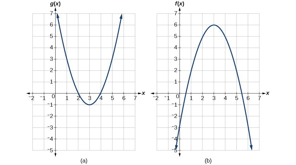
Figure 3
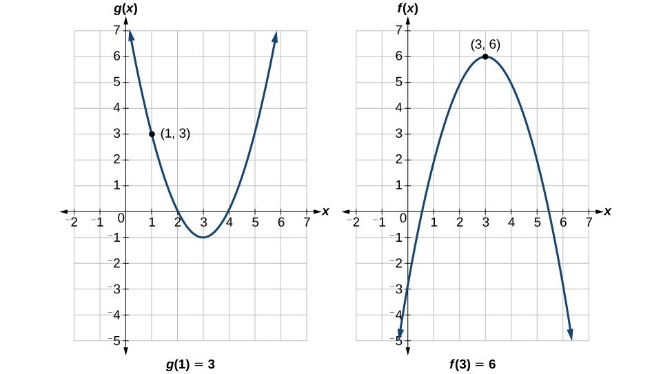
Figure 4
To evaluate [latex]f\left(g\left(1\right)\right)[/latex], we start with the inside evaluation.
We evaluate [latex]g\left(1\right)[/latex] using the graph of [latex]g\left(x\right)[/latex], finding the input of 1 on the [latex]x\text{-}[/latex] axis and finding the output value of the graph at that input. Here, [latex]g\left(1\right)=3[/latex]. We use this value as the input to the function [latex]f[/latex].
We can then evaluate the composite function by looking to the graph of [latex]f\left(x\right)[/latex], finding the input of 3 on the [latex]x\text{-}[/latex] axis and reading the output value of the graph at this input. Here, [latex]f\left(3\right)=6[/latex], so [latex]f\left(g\left(1\right)\right)=6[/latex].
Figure 5 shows how we can mark the graphs with arrows to trace the path from the input value to the output value.
Figure 5
When evaluating a composite function where we have either created or been given formulas, the rule of working from the inside out remains the same. The input value to the outer function will be the output of the inner function, which may be a numerical value, a variable name, or a more complicated expression.
While we can compose the functions for each individual input value, it is sometimes helpful to find a single formula that will calculate the result of a composition [latex]f\left(g\left(x\right)\right)[/latex]. To do this, we will extend our idea of function evaluation. Recall that, when we evaluate a function like [latex]f\left(t\right)={t}^{2}-t[/latex], we substitute the value inside the parentheses into the formula wherever we see the input variable.
Given [latex]f\left(t\right)={t}^{2}-{t}[/latex] and [latex]h\left(x\right)=3x+2[/latex], evaluate [latex]f\left(h\left(1\right)\right)[/latex].
Because the inside expression is [latex]h\left(1\right)[/latex], we start by evaluating [latex]h\left(x\right)[/latex] at 1.
Then [latex]f\left(h\left(1\right)\right)=f\left(5\right)[/latex], so we evaluate [latex]f\left(t\right)[/latex] at an input of 5.
It makes no difference what the input variables [latex]t[/latex] and [latex]x[/latex] were called in this problem because we evaluated for specific numerical values.
Given [latex]f\left(t\right)={t}^{2}-t[/latex] and [latex]h\left(x\right)=3x+2[/latex], evaluate
A) [latex]h\left(f\left(2\right)\right)[/latex]
B) [latex]h\left(f\left(-2\right)\right)[/latex]
As we discussed previously, the domain of a composite function such as [latex]f\circ g[/latex] is dependent on the domain of [latex]g[/latex] and the domain of [latex]f[/latex]. It is important to know when we can apply a composite function and when we cannot, that is, to know the domain of a function such as [latex]f\circ g[/latex]. Let us assume we know the domains of the functions [latex]f[/latex] and [latex]g[/latex] separately. If we write the composite function for an input [latex]x[/latex] as [latex]f\left(g\left(x\right)\right)[/latex], we can see right away that [latex]x[/latex] must be a member of the domain of [latex]g[/latex] in order for the expression to be meaningful, because otherwise we cannot complete the inner function evaluation. However, we also see that [latex]g\left(x\right)[/latex] must be a member of the domain of [latex]f[/latex], otherwise the second function evaluation in [latex]f\left(g\left(x\right)\right)[/latex] cannot be completed, and the expression is still undefined. Thus the domain of [latex]f\circ g[/latex] consists of only those inputs in the domain of [latex]g[/latex] that produce outputs from [latex]g[/latex] belonging to the domain of [latex]f[/latex]. Note that the domain of [latex]f[/latex] composed with [latex]g[/latex] is the set of all [latex]x[/latex] such that [latex]x[/latex] is in the domain of [latex]g[/latex] and [latex]g\left(x\right)[/latex] is in the domain of [latex]f[/latex].
The domain of a composite function [latex]f\left(g\left(x\right)\right)[/latex] is the set of those inputs [latex]x[/latex] in the domain of [latex]g[/latex] for which [latex]g\left(x\right)[/latex] is in the domain of [latex]f[/latex].
Find the domain of
The domain of [latex]g\left(x\right)\\[/latex] consists of all real numbers except [latex]x=\frac{2}{3}\\[/latex], since that input value would cause us to divide by 0. Likewise, the domain of [latex]f[/latex] consists of all real numbers except 1. So we need to exclude from the domain of [latex]g\left(x\right)\\[/latex] that value of [latex]x[/latex] for which [latex]g\left(x\right)=1\\[/latex].
So the domain of [latex]f\circ g[/latex] is the set of all real numbers except [latex]\frac{2}{3}\\[/latex] and [latex]2[/latex]. This means that
We can write this in interval notation as
Find the domain of
Because we cannot take the square root of a negative number, the domain of [latex]g[/latex] is [latex]\left(-\infty ,3\right]\\[/latex]. Now we check the domain of the composite function
The domain of this function is [latex]\left(-\infty ,5\right]\\[/latex]. To find the domain of [latex]f\circ g\\[/latex], we ask ourselves if there are any further restrictions offered by the domain of the composite function. The answer is no, since [latex]\left(-\infty ,3\right]\\[/latex] is a proper subset of the domain of [latex]f\circ g\\[/latex]. This means the domain of [latex]f\circ g\\[/latex] is the same as the domain of [latex]g[/latex], namely, [latex]\left(-\infty ,3\right]\\[/latex].
This example shows that knowledge of the range of functions (specifically the inner function) can also be helpful in finding the domain of a composite function. It also shows that the domain of [latex]f\circ g[/latex] can contain values that are not in the domain of [latex]f[/latex], though they must be in the domain of [latex]g[/latex].
Find the domain of
In some cases, it is necessary to decompose a complicated function. In other words, we can write it as a composition of two simpler functions. There may be more than one way to decompose a composite function, so we may choose the decomposition that appears to be most expedient.
Write [latex]f\left(x\right)=\sqrt{5-{x}^{2}}\\[/latex] as the composition of two functions.
We are looking for two functions, [latex]g\\[/latex] and [latex]h\\[/latex], so [latex]f\left(x\right)=g\left(h\left(x\right)\right)\\[/latex]. To do this, we look for a function inside a function in the formula for [latex]f\left(x\right)\\[/latex]. As one possibility, we might notice that the expression [latex]5-{x}^{2}\\[/latex] is the inside of the square root. We could then decompose the function as
We can check our answer by recomposing the functions.
Write [latex]f\left(x\right)=\frac{4}{3-\sqrt{4+{x}^{2}}}\\[/latex] as the composition of two functions.
| Composite function | [latex]\left(f\circ g\right)\left(x\right)=f\left(g\left(x\right)\right)\\[/latex] |
1. How does one find the domain of the quotient of two functions, [latex]\frac{f}{g}?\\[/latex]
2. What is the composition of two functions, [latex]f\circ g?[/latex]
3. If the order is reversed when composing two functions, can the result ever be the same as the answer in the original order of the composition? If yes, give an example. If no, explain why not.
4. How do you find the domain for the composition of two functions, [latex]f\circ g?[/latex]
5. Given [latex]f\left(x\right)={x}^{2}+2x\text{ }[/latex] and [latex] g\left(x\right)=6-{x}^{2}[/latex], find [latex]f+g,f-g,fg,\text{ }[/latex] and [latex]\text{ }\frac{f}{g}\\[/latex]. Determine the domain for each function in interval notation.
6. Given [latex]f\left(x\right)=-3{x}^{2}+x\text{ }[/latex] and [latex]\text{ }g\left(x\right)=5[/latex], find [latex]f+g,f-g,fg[/latex], and [latex]\text{ }\frac{f}{g}\\[/latex]. Determine the domain for each function in interval notation.
7. Given [latex]f\left(x\right)=2{x}^{2}+4x\text{ }[/latex] and [latex]\text{ }g\left(x\right)=\frac{1}{2x}\\[/latex], find [latex]f+g,f-g,fg,\text{ }[/latex] and [latex]\text{ }\frac{f}{g}\\[/latex]. Determine the domain for each function in interval notation.
8. Given [latex]f\left(x\right)=\frac{1}{x - 4}\\[/latex] and [latex]g\left(x\right)=\frac{1}{6-x}\\[/latex], find [latex]f+g,f-g,fg,\text{ }[/latex] and [latex]\text{ }\frac{f}{g}\\[/latex]. Determine the domain for each function in interval notation.
9. Given [latex]f\left(x\right)=3{x}^{2}\\[/latex] and [latex]g\left(x\right)=\sqrt{x - 5}\\[/latex], find [latex]f+g,f-g,fg,\text{ }\\[/latex] and [latex]\text{ }\frac{f}{g}\\[/latex]. Determine the domain for each function in interval notation.
10. Given [latex]f\left(x\right)=\sqrt{x}\\[/latex] and [latex]g\left(x\right)=|x - 3|\\[/latex], find [latex]\frac{g}{f}\\[/latex]. Determine the domain of the function in interval notation.
11. Given [latex]f\left(x\right)=2{x}^{2}+1\\[/latex] and [latex]g\left(x\right)=3x - 5\\[/latex], find the following:
[latex]f\left(g\left(2\right)\right)\\[/latex]
[latex]f\left(g\left(x\right)\right)\\[/latex]
[latex]g\left(f\left(x\right)\right)\\[/latex]
[latex]\left(g\circ g\right)\left(x\right)\\[/latex]
[latex]\left(f\circ f\right)\left(-2\right)\\[/latex]
For the following exercises, use each pair of functions to find [latex]f\left(g\left(x\right)\right)\\[/latex] and [latex]g\left(f\left(x\right)\right)\\[/latex]. Simplify your answers.
12. [latex]f\left(x\right)={x}^{2}+1,g\left(x\right)=\sqrt{x+2}\\[/latex]
13. [latex]f\left(x\right)=\sqrt{x}+2,g\left(x\right)={x}^{2}+3\\[/latex]
14. [latex]f\left(x\right)=|x|,g\left(x\right)=5x+1\\[/latex]
15. [latex]f\left(x\right)=\sqrt[3]{x},g\left(x\right)=\frac{x+1}{{x}^{3}}\\[/latex]
16. [latex]f\left(x\right)=\frac{1}{x - 6},g\left(x\right)=\frac{7}{x}+6\\[/latex]
17. [latex]f\left(x\right)=\frac{1}{x - 4},g\left(x\right)=\frac{2}{x}+4\\[/latex]
For the following exercises, use each set of functions to find [latex]f\left(g\left(h\left(x\right)\right)\right)\\[/latex]. Simplify your answers.
18. [latex]f\left(x\right)={x}^{4}+6[/latex], [latex]g\left(x\right)=x - 6[/latex], and [latex]h\left(x\right)=\sqrt{x}\\[/latex]
19. [latex]f\left(x\right)={x}^{2}+1[/latex], [latex]g\left(x\right)=\frac{1}{x}[/latex], and [latex]h\left(x\right)=x+3\\[/latex]
20. Given [latex]f\left(x\right)=\frac{1}{x}[/latex] and [latex]g\left(x\right)=x - 3\\[/latex], find the following:
[latex]\left(f\circ g\right)\left(x\right)\\[/latex]
the domain of [latex]\left(f\circ g\right)\left(x\right)\\[/latex] in interval notation
[latex]\left(g\circ f\right)\left(x\right)\\[/latex]
the domain of [latex]\left(g\circ f\right)\left(x\right)\\[/latex]
[latex]\left(\frac{f}{g}\right)x\\[/latex]
21. Given [latex]f\left(x\right)=\sqrt{2 - 4x}\\[/latex] and [latex]g\left(x\right)=-\frac{3}{x}\\[/latex], find the following:
a. [latex]\left(g\circ f\right)\left(x\right)\\[/latex]
b. the domain of [latex]\left(g\circ f\right)\left(x\right)\\[/latex] in interval notation
22. Given the functions [latex]f\left(x\right)=\frac{1-x}{x}\text{and}g\left(x\right)=\frac{1}{1+{x}^{2}}\\[/latex], find the following:
a. [latex]\left(g\circ f\right)\left(x\right)\\[/latex]
b. [latex]\left(g\circ f\right)\left(\text{2}\right)\\[/latex]
23. Given functions [latex]p\left(x\right)=\frac{1}{\sqrt{x}}\\[/latex] and [latex]m\left(x\right)={x}^{2}-4\\[/latex], state the domain of each of the following functions using interval notation:
[latex]\frac{p\left(x\right)}{m\left(x\right)}\\[/latex]
[latex]p\left(m\left(x\right)\right)\\[/latex]
[latex]m\left(p\left(x\right)\right)\\[/latex]
24. Given functions [latex]q\left(x\right)=\frac{1}{\sqrt{x}}\\[/latex] and [latex]h\left(x\right)={x}^{2}-9\\[/latex], state the domain of each of the following functions using interval notation.
[latex]\frac{q\left(x\right)}{h\left(x\right)}\\[/latex]
[latex]q\left(h\left(x\right)\right)\\[/latex]
[latex]h\left(q\left(x\right)\right)\\[/latex]
25. For [latex]f\left(x\right)=\frac{1}{x}\\[/latex] and [latex]g\left(x\right)=\sqrt{x - 1}\\[/latex], write the domain of [latex]\left(f\circ g\right)\left(x\right)\\[/latex] in interval notation.
For the following exercises, find functions [latex]f\left(x\right)\\[/latex] and [latex]g\left(x\right)\\[/latex] so the given function can be expressed as [latex]h\left(x\right)=f\left(g\left(x\right)\right)\\[/latex].
26. [latex]h\left(x\right)={\left(x+2\right)}^{2}\\[/latex]
27. [latex]h\left(x\right)={\left(x - 5\right)}^{3}\\[/latex]
28. [latex]h\left(x\right)=\frac{3}{x - 5}\\[/latex]
29. [latex]h\left(x\right)=\frac{4}{{\left(x+2\right)}^{2}}\\[/latex]
30. [latex]h\left(x\right)=4+\sqrt[3]{x}\\[/latex]
31. [latex]h\left(x\right)=\sqrt[3]{\frac{1}{2x - 3}}\\[/latex]
32. [latex]h\left(x\right)=\frac{1}{{\left(3{x}^{2}-4\right)}^{-3}}\\[/latex]
33. [latex]h\left(x\right)=\sqrt[4]{\frac{3x - 2}{x+5}}\\[/latex]
34. [latex]h\left(x\right)={\left(\frac{8+{x}^{3}}{8-{x}^{3}}\right)}^{4}\\[/latex]
35. [latex]h\left(x\right)=\sqrt{2x+6}\\[/latex]
36. [latex]h\left(x\right)={\left(5x - 1\right)}^{3}\\[/latex]
37. [latex]h\left(x\right)=\sqrt[3]{x - 1}\\[/latex]
38. [latex]h\left(x\right)=\left|{x}^{2}+7\right|\\[/latex]
39. [latex]h\left(x\right)=\frac{1}{{\left(x - 2\right)}^{3}}\\[/latex]
40. [latex]h\left(x\right)={\left(\frac{1}{2x - 3}\right)}^{2}\\[/latex]
41. [latex]h\left(x\right)=\sqrt{\frac{2x - 1}{3x+4}}\\[/latex]
For the following exercises, use the graphs of [latex]f[/latex] and [latex]g[/latex] to evaluate the expressions.


42. [latex]f\left(g\left(3\right)\right)[/latex]
43. [latex]f\left(g\left(1\right)\right)[/latex]
44. [latex]g\left(f\left(1\right)\right)[/latex]
45. [latex]g\left(f\left(0\right)\right)[/latex]
46. [latex]f\left(f\left(5\right)\right)[/latex]
47. [latex]f\left(f\left(4\right)\right)[/latex]
48. [latex]g\left(g\left(2\right)\right)[/latex]
49. [latex]g\left(g\left(0\right)\right)[/latex]
For the following exercises, use graphs of [latex]f\left(x\right)[/latex] [latex]g\left(x\right)[/latex], and [latex]h\left(x\right)[/latex], to evaluate the expressions.


50. [latex]g\left(f\left(1\right)\right)[/latex]
51. [latex]g\left(f\left(2\right)\right)[/latex]
52. [latex]f\left(g\left(4\right)\right)[/latex]
53. [latex]f\left(g\left(1\right)\right)[/latex]
54. [latex]f\left(h\left(2\right)\right)[/latex]
55. [latex]h\left(f\left(2\right)\right)[/latex]
56. [latex]f\left(g\left(h\left(4\right)\right)\right)[/latex]
57. [latex]f\left(g\left(f\left(-2\right)\right)\right)[/latex]
For the following exercises, use the function values for [latex]f\text{ and }g[/latex] to evaluate each expression.
| [latex]x[/latex] | [latex]f\left(x\right)[/latex] | [latex]g\left(x\right)[/latex] |
| 0 | 7 | 9 |
| 1 | 6 | 5 |
| 2 | 5 | 6 |
| 3 | 8 | 2 |
| 4 | 4 | 1 |
| 5 | 0 | 8 |
| 6 | 2 | 7 |
| 7 | 1 | 3 |
| 8 | 9 | 4 |
| 9 | 3 | 0 |
58. [latex]f\left(g\left(8\right)\right)[/latex]
59. [latex]f\left(g\left(5\right)\right)[/latex]
60. [latex]g\left(f\left(5\right)\right)[/latex]
61. [latex]g\left(f\left(3\right)\right)[/latex]
62. [latex]f\left(f\left(4\right)\right)[/latex]
63. [latex]f\left(f\left(1\right)\right)[/latex]
64. [latex]g\left(g\left(2\right)\right)[/latex]
65. [latex]g\left(g\left(6\right)\right)[/latex]
For the following exercises, use the function values for [latex]f\text{ and }g[/latex] to evaluate the expressions.
| [latex]x[/latex] | [latex]f\left(x\right)[/latex] | [latex]g\left(x\right)[/latex] |
| -3 | 11 | -8 |
| -2 | 9 | -3 |
| -1 | 7 | 0 |
| 0 | 5 | 1 |
| 1 | 3 | 0 |
| 2 | 1 | -3 |
| 3 | -1 | -8 |
66. [latex]\left(f\circ g\right)\left(1\right)[/latex]
67. [latex]\left(f\circ g\right)\left(2\right)[/latex]
68. [latex]\left(g\circ f\right)\left(2\right)[/latex]
69. [latex]\left(g\circ f\right)\left(3\right)[/latex]
70. [latex]\left(g\circ g\right)\left(1\right)[/latex]
71. [latex]\left(f\circ f\right)\left(3\right)[/latex]
For the following exercises, use each pair of functions to find [latex]f\left(g\left(0\right)\right)[/latex] and [latex]g\left(f\left(0\right)\right)[/latex].
72. [latex]f\left(x\right)=4x+8,g\left(x\right)=7-{x}^{2}\\[/latex]
73. [latex]f\left(x\right)=5x+7,g\left(x\right)=4 - 2{x}^{2}\\[/latex]
74. [latex]f\left(x\right)=\sqrt{x+4},g\left(x\right)=12-{x}^{3}\\[/latex]
75. [latex]f\left(x\right)=\frac{1}{x+2},g\left(x\right)=4x+3\\[/latex]
For the following exercises, use the functions [latex]f\left(x\right)=2{x}^{2}+1\\[/latex] and [latex]g\left(x\right)=3x+5\\[/latex] to evaluate or find the composite function as indicated.
76. [latex]f\left(g\left(2\right)\right)[/latex]
77. [latex]f\left(g\left(x\right)\right)[/latex]
78. [latex]g\left(f\left(-3\right)\right)[/latex]
79. [latex]\left(g\circ g\right)\left(x\right)[/latex]
For the following exercises, use [latex]f\left(x\right)={x}^{3}+1[/latex] and [latex]g\left(x\right)=\sqrt[3]{x - 1}\\[/latex].
80. Find [latex]\left(f\circ g\right)\left(x\right)[/latex] and [latex]\left(g\circ f\right)\left(x\right)[/latex]. Compare the two answers.
81. Find [latex]\left(f\circ g\right)\left(2\right)[/latex] and [latex]\left(g\circ f\right)\left(2\right)[/latex].
82. What is the domain of [latex]\left(g\circ f\right)\left(x\right)?[/latex]
83. What is the domain of [latex]\left(f\circ g\right)\left(x\right)?[/latex]
84. Let [latex]f\left(x\right)=\frac{1}{x}\\[/latex].
a. Find [latex]\left(f\circ f\right)\left(x\right)[/latex].
b. Is [latex]\left(f\circ f\right)\left(x\right)[/latex] for any function [latex]f[/latex] the same result as the answer to part (a) for any function? Explain.
For the following exercises, let [latex]F\left(x\right)={\left(x+1\right)}^{5}[/latex], [latex]f\left(x\right)={x}^{5}[/latex], and [latex]g\left(x\right)=x+1[/latex].
85. True or False: [latex]\left(g\circ f\right)\left(x\right)=F\left(x\right)[/latex].
86. True or False: [latex]\left(f\circ g\right)\left(x\right)=F\left(x\right)[/latex].
For the following exercises, find the composition when [latex]f\left(x\right)={x}^{2}+2[/latex] for all [latex]x\ge 0[/latex] and [latex]g\left(x\right)=\sqrt{x - 2}[/latex].
87. [latex]\left(f\circ g\right)\left(6\right);\left(g\circ f\right)\left(6\right)[/latex]
88. [latex]\left(g\circ f\right)\left(a\right);\left(f\circ g\right)\left(a\right)[/latex]
89. [latex]\left(f\circ g\right)\left(11\right);\left(g\circ f\right)\left(11\right)[/latex]
90. The function [latex]D\left(p\right)[/latex] gives the number of items that will be demanded when the price is [latex]p[/latex]. The production cost [latex]C\left(x\right)[/latex] is the cost of producing [latex]x[/latex] items. To determine the cost of production when the price is $6, you would do which of the following?
a. Evaluate [latex]D\left(C\left(6\right)\right)[/latex].
b. Evaluate [latex]C\left(D\left(6\right)\right)[/latex].
c. Solve [latex]D\left(C\left(x\right)\right)=6[/latex].
d. Solve [latex]C\left(D\left(p\right)\right)=6[/latex].
91. The function [latex]A\left(d\right)[/latex] gives the pain level on a scale of 0 to 10 experienced by a patient with [latex]d[/latex] milligrams of a pain-reducing drug in her system. The milligrams of the drug in the patient’s system after [latex]t[/latex] minutes is modeled by [latex]m\left(t\right)[/latex]. Which of the following would you do in order to determine when the patient will be at a pain level of 4?
a. Evaluate [latex]A\left(m\left(4\right)\right)[/latex].
b. Evaluate [latex]m\left(A\left(4\right)\right)[/latex].
c. Solve [latex]A\left(m\left(t\right)\right)=4[/latex].
d. Solve [latex]m\left(A\left(d\right)\right)=4[/latex].
92. A store offers customers a 30% discount on the price [latex]x[/latex] of selected items. Then, the store takes off an additional 15% at the cash register. Write a price function [latex]P\left(x\right)[/latex] that computes the final price of the item in terms of the original price [latex]x[/latex]. (Hint: Use function composition to find your answer.)
93. A rain drop hitting a lake makes a circular ripple. If the radius, in inches, grows as a function of time in minutes according to [latex]r\left(t\right)=25\sqrt{t+2}[/latex], find the area of the ripple as a function of time. Find the area of the ripple at [latex]t=2[/latex].
94. A forest fire leaves behind an area of grass burned in an expanding circular pattern. If the radius of the circle of burning grass is increasing with time according to the formula [latex]r\left(t\right)=2t+1[/latex], express the area burned as a function of time, [latex]t[/latex] (minutes).
95. Use the function you found in the previous exercise to find the total area burned after 5 minutes.
96. The radius [latex]r[/latex], in inches, of a spherical balloon is related to the volume, [latex]V[/latex], by [latex]r\left(V\right)=\sqrt[3]{\frac{3V}{4\pi }}\\[/latex]. Air is pumped into the balloon, so the volume after [latex]t[/latex] seconds is given by [latex]V\left(t\right)=10+20t[/latex].
a. Find the composite function [latex]r\left(V\left(t\right)\right)[/latex].
b. Find the exact time when the radius reaches 10 inches.
97. The number of bacteria in a refrigerated food product is given by [latex]N\left(T\right)=23{T}^{2}-56T+1[/latex], [latex]3<T<33[/latex], where [latex]T[/latex] is the temperature of the food. When the food is removed from the refrigerator, the temperature is given by [latex]T\left(t\right)=5t+1.5[/latex], where [latex]t[/latex] is the time in hours.
a. Find the composite function [latex]N\left(T\left(t\right)\right)[/latex].
b. Find the time (round to two decimal places) when the bacteria count reaches 6752.
1. [latex]\begin{cases}\left(fg\right)\left(x\right)=f\left(x\right)g\left(x\right)=\left(x - 1\right)\left({x}^{2}-1\right)={x}^{3}-{x}^{2}-x+1\\ \left(f-g\right)\left(x\right)=f\left(x\right)-g\left(x\right)=\left(x - 1\right)-\left({x}^{2}-1\right)=x-{x}^{2}\end{cases}[/latex]
No, the functions are not the same.
2. A gravitational force is still a force, so [latex]a\left(G\left(r\right)\right)[/latex] makes sense as the acceleration of a planet at a distance r from the Sun (due to gravity), but [latex]G\left(a\left(F\right)\right)[/latex] does not make sense.
3. [latex]f\left(g\left(1\right)\right)=f\left(3\right)=3[/latex] and [latex]g\left(f\left(4\right)\right)=g\left(1\right)=3[/latex]
4. [latex]g\left(f\left(2\right)\right)=g\left(5\right)=3[/latex]
5. A. 8; B. 20
6. [latex]\left[-4,0\right)\cup \left(0,\infty \right)[/latex]
7. Possible answer:
[latex]g\left(x\right)=\sqrt{4+{x}^{2}}[/latex]
[latex]h\left(x\right)=\frac{4}{3-x}[/latex]
[latex]f=h\circ g[/latex]
1. Find the numbers that make the function in the denominator [latex]g[/latex] equal to zero, and check for any other domain restrictions on [latex]f[/latex] and [latex]g[/latex], such as an even-indexed root or zeros in the denominator.
3. Yes. Sample answer: Let [latex]f\left(x\right)=x+1\text{ and }g\left(x\right)=x - 1[/latex]. Then [latex]f\left(g\left(x\right)\right)=f\left(x - 1\right)=\left(x - 1\right)+1=x[/latex] and [latex]g\left(f\left(x\right)\right)=g\left(x+1\right)=\left(x+1\right)-1=x[/latex]. So [latex]f\circ g=g\circ f[/latex].
5. [latex]\left(f+g\right)\left(x\right)=2x+6[/latex], domain: [latex]\left(-\infty ,\infty \right)[/latex]
[latex]\left(f-g\right)\left(x\right)=2{x}^{2}+2x - 6[/latex], domain: [latex]\left(-\infty ,\infty \right)[/latex]
[latex]\left(fg\right)\left(x\right)=-{x}^{4}-2{x}^{3}+6{x}^{2}+12x[/latex], domain: [latex]\left(-\infty ,\infty \right)[/latex]
[latex]\left(\frac{f}{g}\right)\left(x\right)=\frac{{x}^{2}+2x}{6-{x}^{2}}[/latex], domain: [latex]\left(-\infty ,-\sqrt{6}\right)\cup \left(-\sqrt{6},\sqrt{6}\right)\cup \left(\sqrt{6},\infty \right)[/latex]
7. [latex]\left(f+g\right)\left(x\right)=\frac{4{x}^{3}+8{x}^{2}+1}{2x}[/latex], domain: [latex]\left(-\infty ,0\right)\cup \left(0,\infty \right)[/latex]
[latex]\left(f-g\right)\left(x\right)=\frac{4{x}^{3}+8{x}^{2}-1}{2x}[/latex], domain: [latex]\left(-\infty ,0\right)\cup \left(0,\infty \right)[/latex]
[latex]\left(fg\right)\left(x\right)=x+2[/latex], domain: [latex]\left(-\infty ,0\right)\cup \left(0,\infty \right)[/latex]
[latex]\left(\frac{f}{g}\right)\left(x\right)=4{x}^{3}+8{x}^{2}[/latex], domain: [latex]\left(-\infty ,0\right)\cup \left(0,\infty \right)[/latex]
9. [latex]\left(f+g\right)\left(x\right)=3{x}^{2}+\sqrt{x - 5}[/latex], domain: [latex]\left[5,\infty \right)[/latex]
[latex]\left(f-g\right)\left(x\right)=3{x}^{2}-\sqrt{x - 5}[/latex], domain: [latex]\left[5,\infty \right)[/latex]
[latex]\left(fg\right)\left(x\right)=3{x}^{2}\sqrt{x - 5}[/latex], domain: [latex]\left[5,\infty \right)[/latex]
[latex]\left(\frac{f}{g}\right)\left(x\right)=\frac{3{x}^{2}}{\sqrt{x - 5}}[/latex], domain: [latex]\left(5,\infty \right)[/latex]
11. a. 3; b. [latex]f\left(g\left(x\right)\right)=2{\left(3x - 5\right)}^{2}+1[/latex]; c. [latex]f\left(g\left(x\right)\right)=6{x}^{2}-2[/latex]; d. [latex]\left(g\circ g\right)\left(x\right)=3\left(3x - 5\right)-5=9x - 20[/latex]; e. [latex]\left(f\circ f\right)\left(-2\right)=163[/latex]
13. [latex]f\left(g\left(x\right)\right)=\sqrt{{x}^{2}+3}+2,g\left(f\left(x\right)\right)=x+4\sqrt{x}+7[/latex]
15. [latex]f\left(g\left(x\right)\right)=\sqrt[3]{\frac{x+1}{{x}^{3}}}=\frac{\sqrt[3]{x+1}}{x},g\left(f\left(x\right)\right)=\frac{\sqrt[3]{x}+1}{x}[/latex]
17. [latex]\left(f\circ g\right)\left(x\right)=\frac{1}{\frac{2}{x}+4 - 4}=\frac{x}{2},\text{ }\left(g\circ f\right)\left(x\right)=2x - 4[/latex]
19. [latex]f\left(g\left(h\left(x\right)\right)\right)={\left(\frac{1}{x+3}\right)}^{2}+1[/latex]
21. a. [latex]\left(g\circ f\right)\left(x\right)=-\frac{3}{\sqrt{2 - 4x}}[/latex]; b. [latex]\left(-\infty ,\frac{1}{2}\right)[/latex]
23. a. [latex]\left(0,2\right)\cup \left(2,\infty \right)[/latex]; b. [latex]\left(-\infty ,-2\right)\cup \left(2,\infty \right)[/latex]; c. [latex]\left(0,\infty \right)[/latex]
25. [latex]\left(1,\infty \right)[/latex]
27. sample: [latex]\begin{cases}f\left(x\right)={x}^{3}\\ g\left(x\right)=x - 5\end{cases}[/latex]
29. sample: [latex]\begin{cases}f\left(x\right)=\frac{4}{x}\hfill \\ g\left(x\right)={\left(x+2\right)}^{2}\hfill \end{cases}[/latex]
31. sample: [latex]\begin{cases}f\left(x\right)=\sqrt[3]{x}\\ g\left(x\right)=\frac{1}{2x - 3}\end{cases}[/latex]
33. sample: [latex]\begin{cases}f\left(x\right)=\sqrt[4]{x}\\ g\left(x\right)=\frac{3x - 2}{x+5}\end{cases}[/latex]
35. sample: [latex]f\left(x\right)=\sqrt{x}[/latex]
[latex]g\left(x\right)=2x+6[/latex]
37.sample: [latex]f\left(x\right)=\sqrt[3]{x}[/latex]
[latex]g\left(x\right)=\left(x - 1\right)[/latex]
39. sample: [latex]f\left(x\right)={x}^{3}[/latex]
[latex]g\left(x\right)=\frac{1}{x - 2}[/latex]
41. sample: [latex]f\left(x\right)=\sqrt{x}[/latex]
[latex]g\left(x\right)=\frac{2x - 1}{3x+4}[/latex]
43. 2
45. 5
47. 4
49. 0
51. 2
53. 1
55. 4
57. 4
59. 9
61. 4
63. 2
65. 3
67. 11
69. 0
71. 7
73. [latex]f\left(g\left(0\right)\right)=27,g\left(f\left(0\right)\right)=-94[/latex]
75. [latex]f\left(g\left(0\right)\right)=\frac{1}{5},g\left(f\left(0\right)\right)=5[/latex]
77. [latex]18{x}^{2}+60x+51[/latex]
79. [latex]g\circ g\left(x\right)=9x+20[/latex]
81. 2
83. [latex]\left(-\infty ,\infty \right)[/latex]
85. False
87. [latex]\left(f\circ g\right)\left(6\right)=6[/latex] ; [latex]\left(g\circ f\right)\left(6\right)=6[/latex]
89. [latex]\left(f\circ g\right)\left(11\right)=11,\left(g\circ f\right)\left(11\right)=11[/latex]
91. c. Solve [latex]A\left(m\left(t\right)\right)=4[/latex].
93. [latex]A\left(t\right)=\pi {\left(25\sqrt{t+2}\right)}^{2}[/latex] and [latex]A\left(2\right)=\pi {\left(25\sqrt{4}\right)}^{2}=2500\pi [/latex] square inches
95. [latex]A\left(5\right)=\pi {\left(2\left(5\right)+1\right)}^{2}=121\pi [/latex] square units
97. a. [latex]N\left(T\left(t\right)\right)=23{\left(5t+1.5\right)}^{2}-56\left(5t+1.5\right)+1[/latex];
b. 3.38 hours
By the end of this lesson, you will be able to:
Figure 1. (credit: “Misko”/Flickr)
We all know that a flat mirror enables us to see an accurate image of ourselves and whatever is behind us. When we tilt the mirror, the images we see may shift horizontally or vertically. But what happens when we bend a flexible mirror? Like a carnival funhouse mirror, it presents us with a distorted image of ourselves, stretched or compressed horizontally or vertically. In a similar way, we can distort or transform mathematical functions to better adapt them to describing objects or processes in the real world. In this section, we will take a look at several kinds of transformations.
Often when given a problem, we try to model the scenario using mathematics in the form of words, tables, graphs, and equations. One method we can employ is to adapt the basic graphs of the toolkit functions to build new models for a given scenario. There are systematic ways to alter functions to construct appropriate models for the problems we are trying to solve.
One simple kind of transformation involves shifting the entire graph of a function up, down, right, or left. The simplest shift is a vertical shift, moving the graph up or down, because this transformation involves adding a positive or negative constant to the function. In other words, we add the same constant to the output value of the function regardless of the input. For a function [latex]g\left(x\right)=f\left(x\right)+k\\[/latex], the function [latex]f\left(x\right)\\[/latex] is shifted vertically [latex]k\\[/latex] units.
Figure 2. Vertical shift by [latex]k=1\\[/latex] of the cube root function [latex]f\left(x\right)=\sqrt[3]{x}\\[/latex].
To help you visualize the concept of a vertical shift, consider that [latex]y=f\left(x\right)\\[/latex]. Therefore, [latex]f\left(x\right)+k\\[/latex] is equivalent to [latex]y+k\\[/latex]. Every unit of [latex]y[/latex] is replaced by [latex]y+k\\[/latex], so the [latex]y\text{-}\\[/latex] value increases or decreases depending on the value of [latex]k\\[/latex]. The result is a shift upward or downward.
Given a function [latex]f\left(x\right)\\[/latex], a new function [latex]g\left(x\right)=f\left(x\right)+k\\[/latex], where [latex]k[/latex] is a constant, is a vertical shift of the function [latex]f\left(x\right)\\[/latex]. All the output values change by [latex]k[/latex] units. If [latex]k[/latex] is positive, the graph will shift up. If [latex]k[/latex] is negative, the graph will shift down.
To regulate temperature in a green building, airflow vents near the roof open and close throughout the day. Figure 2 shows the area of open vents [latex]V[/latex] (in square feet) throughout the day in hours after midnight, [latex]t[/latex]. During the summer, the facilities manager decides to try to better regulate temperature by increasing the amount of open vents by 20 square feet throughout the day and night. Sketch a graph of this new function.
Figure 3
We can sketch a graph of this new function by adding 20 to each of the output values of the original function. This will have the effect of shifting the graph vertically up, as shown in Figure 4.
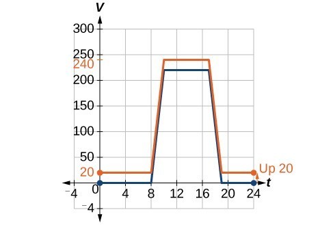
Figure 4
Notice that for each input value, the output value has increased by 20, so if we call the new function [latex]S\left(t\right)[/latex], we could write
This notation tells us that, for any value of [latex]t,S\left(t\right)\\[/latex] can be found by evaluating the function [latex]V[/latex] at the same input and then adding 20 to the result. This defines [latex]S[/latex] as a transformation of the function [latex]V[/latex], in this case a vertical shift up 20 units. Notice that, with a vertical shift, the input values stay the same and only the output values change.
| [latex]t[/latex] | 0 | 8 | 10 | 17 | 19 | 24 |
| [latex]V\left(t\right)[/latex] | 0 | 0 | 220 | 220 | 0 | 0 |
| [latex]S\left(t\right)[/latex] | 20 | 20 | 240 | 240 | 20 | 20 |
A function [latex]f\left(x\right)\\[/latex] is given below. Create a table for the function [latex]g\left(x\right)=f\left(x\right)-3\\[/latex].
| [latex]x[/latex] | 2 | 4 | 6 | 8 |
| [latex]f\left(x\right)[/latex] | 1 | 3 | 7 | 11 |
The formula [latex]g\left(x\right)=f\left(x\right)-3\\[/latex] tells us that we can find the output values of [latex]g[/latex] by subtracting 3 from the output values of [latex]f[/latex]. For example:
Subtracting 3 from each [latex]f\left(x\right)[/latex] value, we can complete a table of values for [latex]g\left(x\right)\\[/latex].
| [latex]x[/latex] | 2 | 4 | 6 | 8 |
| [latex]f\left(x\right)[/latex] | 1 | 3 | 7 | 11 |
| [latex]g\left(x\right)[/latex] | −2 | 0 | 4 | 8 |
As with the earlier vertical shift, notice the input values stay the same and only the output values change.
The function [latex]h\left(t\right)=-4.9{t}^{2}+30t\\[/latex] gives the height [latex]h[/latex] of a ball (in meters) thrown upward from the ground after [latex]t[/latex] seconds. Suppose the ball was instead thrown from the top of a 10-m building. Relate this new height function [latex]b\left(t\right)[/latex] to [latex]h\left(t\right)\\[/latex], and then find a formula for [latex]b\left(t\right)\\[/latex].
We just saw that the vertical shift is a change to the output, or outside, of the function. We will now look at how changes to input, on the inside of the function, change its graph and meaning. A shift to the input results in a movement of the graph of the function left or right in what is known as a horizontal shift.
Figure 5. Horizontal shift of the function [latex]f\left(x\right)=\sqrt[3]{x}\\[/latex]. Note that [latex]h=+1[/latex] shifts the graph to the left, that is, towards negative values of [latex]x[/latex].
For example, if [latex]f\left(x\right)={x}^{2}\\[/latex], then [latex]g\left(x\right)={\left(x - 2\right)}^{2}\\[/latex] is a new function. Each input is reduced by 2 prior to squaring the function. The result is that the graph is shifted 2 units to the right, because we would need to increase the prior input by 2 units to yield the same output value as given in [latex]f[/latex].
Given a function [latex]f[/latex], a new function [latex]g\left(x\right)=f\left(x-h\right)\\[/latex], where [latex]h[/latex] is a constant, is a horizontal shift of the function [latex]f[/latex]. If [latex]h[/latex] is positive, the graph will shift right. If [latex]h[/latex] is negative, the graph will shift left.
Returning to our building airflow example from Example 2, suppose that in autumn the facilities manager decides that the original venting plan starts too late, and wants to begin the entire venting program 2 hours earlier. Sketch a graph of the new function.
We can set [latex]V\left(t\right)[/latex] to be the original program and [latex]F\left(t\right)[/latex] to be the revised program.
In the new graph, at each time, the airflow is the same as the original function [latex]V[/latex] was 2 hours later. For example, in the original function [latex]V[/latex], the airflow starts to change at 8 a.m., whereas for the function [latex]F[/latex], the airflow starts to change at 6 a.m. The comparable function values are [latex]V\left(8\right)=F\left(6\right)\\[/latex]. Notice also that the vents first opened to [latex]220{\text{ ft}}^{2}\\[/latex] at 10 a.m. under the original plan, while under the new plan the vents reach [latex]220{\text{ ft}}^{\text{2}}\\[/latex] at 8 a.m., so [latex]V\left(10\right)=F\left(8\right)\\[/latex].
Figure 6
In both cases, we see that, because [latex]F\left(t\right)\\[/latex] starts 2 hours sooner, [latex]h=-2[/latex]. That means that the same output values are reached when [latex]F\left(t\right)=V\left(t-\left(-2\right)\right)=V\left(t+2\right)\\[/latex].
Note that [latex]V\left(t+2\right)\\[/latex] has the effect of shifting the graph to the left.
Horizontal changes or “inside changes” affect the domain of a function (the input) instead of the range and often seem counterintuitive. The new function [latex]F\left(t\right)\\[/latex] uses the same outputs as [latex]V\left(t\right)\\[/latex], but matches those outputs to inputs 2 hours earlier than those of [latex]V\left(t\right)\\[/latex]. Said another way, we must add 2 hours to the input of [latex]V[/latex] to find the corresponding output for [latex]F:F\left(t\right)=V\left(t+2\right)\\[/latex].
A function [latex]f\left(x\right)\\[/latex] is given below. Create a table for the function [latex]g\left(x\right)=f\left(x - 3\right)\\[/latex].
| [latex]x[/latex] | 2 | 4 | 6 | 8 |
| [latex]f\left(x\right)[/latex] | 1 | 3 | 7 | 11 |
The formula [latex]g\left(x\right)=f\left(x - 3\right)\\[/latex] tells us that the output values of [latex]g[/latex] are the same as the output value of [latex]f[/latex] when the input value is 3 less than the original value. For example, we know that [latex]f\left(2\right)=1\\[/latex]. To get the same output from the function [latex]g[/latex], we will need an input value that is 3 larger. We input a value that is 3 larger for [latex]g\left(x\right)[/latex] because the function takes 3 away before evaluating the function [latex]f[/latex].
We continue with the other values to create this table.
| [latex]x[/latex] | 5 | 7 | 9 | 11 |
| [latex]x - 3[/latex] | 2 | 4 | 6 | 8 |
| [latex]f\left(x\right)[/latex] | 1 | 3 | 7 | 11 |
| [latex]g\left(x\right)[/latex] | 1 | 3 | 7 | 11 |
The result is that the function [latex]g\left(x\right)[/latex] has been shifted to the right by 3. Notice the output values for [latex]g\left(x\right)[/latex] remain the same as the output values for [latex]f\left(x\right)[/latex], but the corresponding input values, [latex]x[/latex], have shifted to the right by 3. Specifically, 2 shifted to 5, 4 shifted to 7, 6 shifted to 9, and 8 shifted to 11.
The graph in Figure 7 represents both of the functions. We can see the horizontal shift in each point.
Figure 7
This graph represents a transformation of the toolkit function [latex]f\left(x\right)={x}^{2}\\[/latex]. Relate this new function [latex]g\left(x\right)[/latex] to [latex]f\left(x\right)[/latex], and then find a formula for [latex]g\left(x\right)[/latex].
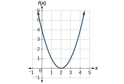
Figure 8
Notice that the graph is identical in shape to the [latex]f\left(x\right)={x}^{2}[/latex] function, but the x-values are shifted to the right 2 units. The vertex used to be at (0,0), but now the vertex is at (2,0). The graph is the basic quadratic function shifted 2 units to the right, so
Notice how we must input the value [latex]x=2[/latex] to get the output value [latex]y=0[/latex]; the x-values must be 2 units larger because of the shift to the right by 2 units. We can then use the definition of the [latex]f\left(x\right)[/latex] function to write a formula for [latex]g\left(x\right)[/latex] by evaluating [latex]f\left(x - 2\right)[/latex].
To determine whether the shift is [latex]+2[/latex] or [latex]-2[/latex] , consider a single reference point on the graph. For a quadratic, looking at the vertex point is convenient. In the original function, [latex]f\left(0\right)=0[/latex]. In our shifted function, [latex]g\left(2\right)=0[/latex]. To obtain the output value of 0 from the function [latex]f[/latex], we need to decide whether a plus or a minus sign will work to satisfy [latex]g\left(2\right)=f\left(x - 2\right)=f\left(0\right)=0\\[/latex]. For this to work, we will need to subtract 2 units from our input values.
The function [latex]G\left(m\right)[/latex] gives the number of gallons of gas required to drive [latex]m[/latex] miles. Interpret [latex]G\left(m\right)+10\\[/latex] and [latex]G\left(m+10\right)\\[/latex].
[latex]G\left(m\right)+10[/latex] can be interpreted as adding 10 to the output, gallons. This is the gas required to drive [latex]m[/latex] miles, plus another 10 gallons of gas. The graph would indicate a vertical shift.
[latex]G\left(m+10\right)[/latex] can be interpreted as adding 10 to the input, miles. So this is the number of gallons of gas required to drive 10 miles more than [latex]m[/latex] miles. The graph would indicate a horizontal shift.
Given the function [latex]f\left(x\right)=\sqrt{x}\\[/latex], graph the original function [latex]f\left(x\right)\\[/latex] and the transformation [latex]g\left(x\right)=f\left(x+2\right)\\[/latex] on the same axes. Is this a horizontal or a vertical shift? Which way is the graph shifted and by how many units?
Another transformation that can be applied to a function is a reflection over the x– or y-axis. A vertical reflection reflects a graph vertically across the x-axis, while a horizontal reflection reflects a graph horizontally across the y-axis. The reflections are shown in Figure 9.
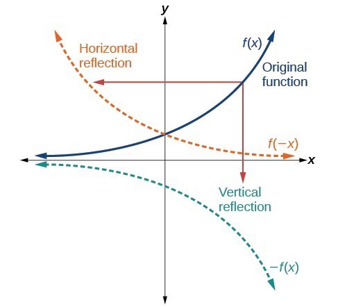
Figure 9. Vertical and horizontal reflections of a function.
Notice that the vertical reflection produces a new graph that is a mirror image of the base or original graph about the x-axis. The horizontal reflection produces a new graph that is a mirror image of the base or original graph about the y-axis.
Given a function [latex]f\left(x\right)\\[/latex], a new function [latex]g\left(x\right)=-f\left(x\right)\\[/latex] is a vertical reflection of the function [latex]f\left(x\right)\\[/latex], sometimes called a reflection about (or over, or through) the x-axis.
Given a function [latex]f\left(x\right)\\[/latex], a new function [latex]g\left(x\right)=f\left(-x\right)\\[/latex] is a horizontal reflection of the function [latex]f\left(x\right)\\[/latex], sometimes called a reflection about the y-axis.
Reflect the graph of [latex]s\left(t\right)=\sqrt{t}\\[/latex] (a) vertically and (b) horizontally.
a. Reflecting the graph vertically means that each output value will be reflected over the horizontal t-axis as shown in Figure 10.
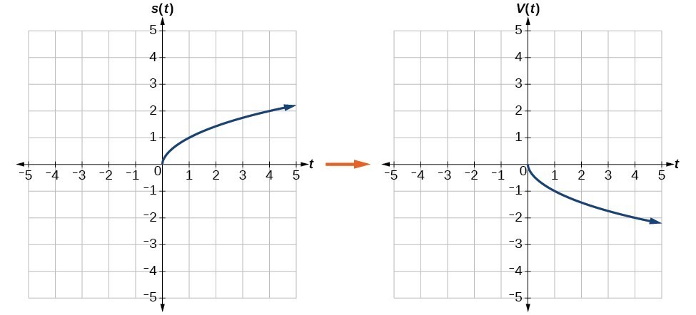
Figure 10. Vertical reflection of the square root function
Because each output value is the opposite of the original output value, we can write
Notice that this is an outside change, or vertical shift, that affects the output [latex]s\left(t\right)\\[/latex] values, so the negative sign belongs outside of the function.
b.
Reflecting horizontally means that each input value will be reflected over the vertical axis as shown in Figure 11.
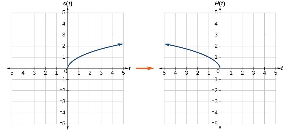
Figure 11. Horizontal reflection of the square root function
Because each input value is the opposite of the original input value, we can write
Notice that this is an inside change or horizontal change that affects the input values, so the negative sign is on the inside of the function.
Note that these transformations can affect the domain and range of the functions. While the original square root function has domain [latex]\left[0,\infty \right)\\[/latex] and range [latex]\left[0,\infty \right)\\[/latex], the vertical reflection gives the [latex]V\left(t\right)\\[/latex] function the range [latex]\left(-\infty ,0\right]\\[/latex] and the horizontal reflection gives the [latex]H\left(t\right)\\[/latex] function the domain [latex]\left(-\infty ,0\right]\\[/latex].
Reflect the graph of [latex]f\left(x\right)=|x - 1|\\[/latex] (a) vertically and (b) horizontally.
A function [latex]f\left(x\right)\\[/latex] is given. Create a table for the functions below.
| [latex]x[/latex] | 2 | 4 | 6 | 8 |
| [latex]f\left(x\right)[/latex] | 1 | 3 | 7 | 11 |
For [latex]g\left(x\right)\\[/latex], the negative sign outside the function indicates a vertical reflection, so the x-values stay the same and each output value will be the opposite of the original output value.
| [latex]x[/latex] | 2 | 4 | 6 | 8 |
| [latex]g\left(x\right)[/latex] | –1 | –3 | –7 | –11 |
For [latex]h\left(x\right)\\[/latex], the negative sign inside the function indicates a horizontal reflection, so each input value will be the opposite of the original input value and the [latex]h\left(x\right)\\[/latex] values stay the same as the [latex]f\left(x\right)\\[/latex] values.
| [latex]x[/latex] | −2 | −4 | −6 | −8 |
| [latex]h\left(x\right)[/latex] | 1 | 3 | 7 | 11 |
| [latex]x[/latex] | −2 | 0 | 2 | 4 |
| [latex]f\left(x\right)[/latex] | 5 | 10 | 15 | 20 |
Using the function [latex]f\left(x\right)\\[/latex] given in the table above, create a table for the functions below.
a. [latex]g\left(x\right)=-f\left(x\right)\\[/latex]
b. [latex]h\left(x\right)=f\left(-x\right)\\[/latex]
Some functions exhibit symmetry so that reflections result in the original graph. For example, horizontally reflecting the toolkit functions [latex]f\left(x\right)={x}^{2}\\[/latex] or [latex]f\left(x\right)=|x|\\[/latex] will result in the original graph. We say that these types of graphs are symmetric about the y-axis. Functions whose graphs are symmetric about the y-axis are called even functions.
If the graphs of [latex]f\left(x\right)={x}^{3}\\[/latex] or [latex]f\left(x\right)=\frac{1}{x}\\[/latex] were reflected over both axes, the result would be the original graph.
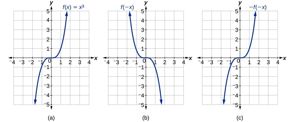
Figure 12. (a) The cubic toolkit function (b) Horizontal reflection of the cubic toolkit function (c) Horizontal and vertical reflections reproduce the original cubic function.
We say that these graphs are symmetric about the origin. A function with a graph that is symmetric about the origin is called an odd function.
Note: A function can be neither even nor odd if it does not exhibit either symmetry. For example, [latex]f\left(x\right)={2}^{x}\\[/latex] is neither even nor odd. Also, the only function that is both even and odd is the constant function [latex]f\left(x\right)=0\\[/latex].
A function is called an even function if for every input [latex]x\\[/latex]
The graph of an even function is symmetric about the [latex]y\text{-}\\[/latex] axis.
A function is called an odd function if for every input [latex]x\\[/latex]
The graph of an odd function is symmetric about the origin.
Is the function [latex]f\left(x\right)={x}^{3}+2x\\[/latex] even, odd, or neither?
Without looking at a graph, we can determine whether the function is even or odd by finding formulas for the reflections and determining if they return us to the original function. Let’s begin with the rule for even functions.
This does not return us to the original function, so this function is not even. We can now test the rule for odd functions.
Because [latex]-f\left(-x\right)=f\left(x\right)\\[/latex], this is an odd function.
Consider the graph of [latex]f\\[/latex]. Notice that the graph is symmetric about the origin. For every point [latex]\left(x,y\right)\\[/latex] on the graph, the corresponding point [latex]\left(-x,-y\right)\\[/latex] is also on the graph. For example, (1, 3) is on the graph of [latex]f\\[/latex], and the corresponding point [latex]\left(-1,-3\right)\\[/latex] is also on the graph.
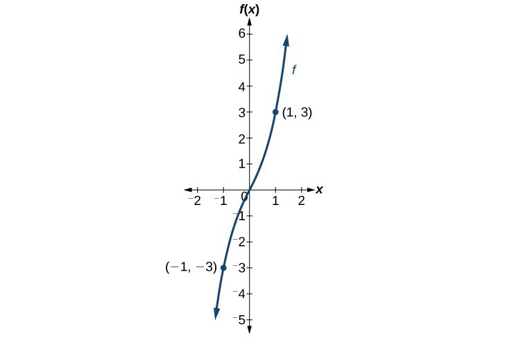
Figure 13
Is the function [latex]f\left(s\right)={s}^{4}+3{s}^{2}+7\\[/latex] even, odd, or neither?
Adding a constant to the inputs or outputs of a function changed the position of a graph with respect to the axes, but it did not affect the shape of a graph. We now explore the effects of multiplying the inputs or outputs by some quantity.
We can transform the inside (input values) of a function or we can transform the outside (output values) of a function. Each change has a specific effect that can be seen graphically.
When we multiply a function by a positive constant, we get a function whose graph is stretched or compressed vertically in relation to the graph of the original function. If the constant is greater than 1, we get a vertical stretch; if the constant is between 0 and 1, we get a vertical compression. The graph below shows a function multiplied by constant factors 2 and 0.5 and the resulting vertical stretch and compression.
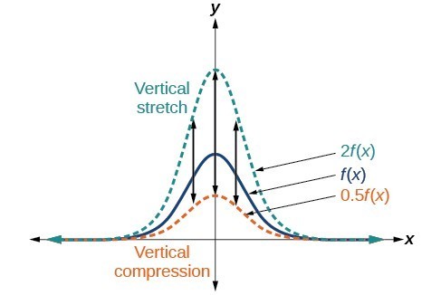
Figure 14. Vertical stretch and compression
Given a function [latex]f\left(x\right)\\[/latex], a new function [latex]g\left(x\right)=af\left(x\right)\\[/latex], where [latex]a\\[/latex] is a constant, is a vertical stretch or vertical compression of the function [latex]f\left(x\right)\\[/latex].
If [latex]a>1\\[/latex], the graph is stretched by a factor of [latex]a\\[/latex].
If [latex]{ 0 }<{ a }<{ 1 }\\[/latex], the graph is compressed by a factor of [latex]a\\[/latex].
If [latex]a<0\\[/latex], the graph is either stretched or compressed and also reflected about the x-axis.
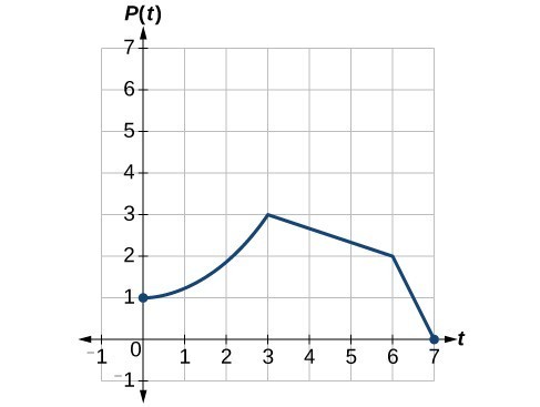
Figure 15
A function [latex]P\left(t\right)\\[/latex] models the population of fruit flies.
A scientist is comparing this population to another population, [latex]Q\\[/latex], whose growth follows the same pattern, but is twice as large. Sketch a graph of this population.
Because the population is always twice as large, the new population’s output values are always twice the original function’s output values.
If we choose four reference points, (0, 1), (3, 3), (6, 2) and (7, 0) we will multiply all of the outputs by 2.
The following shows where the new points for the new graph will be located.
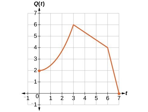
Figure 16
Symbolically, the relationship is written as
This means that for any input [latex]t\\[/latex], the value of the function [latex]Q\\[/latex] is twice the value of the function [latex]P\\[/latex]. Notice that the effect on the graph is a vertical stretching of the graph, where every point doubles its distance from the horizontal axis. The input values, [latex]t\\[/latex], stay the same while the output values are twice as large as before.
A function [latex]f\\[/latex] is given in the table below. Create a table for the function [latex]g\left(x\right)=\frac{1}{2}f\left(x\right)\\[/latex].
| [latex]x[/latex] | 2 | 4 | 6 | 8 |
| [latex]f\left(x\right)[/latex] | 1 | 3 | 7 | 11 |
The formula [latex]g\left(x\right)=\frac{1}{2}f\left(x\right)\\[/latex] tells us that the output values of [latex]g\\[/latex] are half of the output values of [latex]f\\[/latex] with the same inputs. For example, we know that [latex]f\left(4\right)=3\\[/latex]. Then
We do the same for the other values to produce this table.
| [latex]x[/latex] | [latex]2\\[/latex] | [latex]4\\[/latex] | [latex]6\\[/latex] | [latex]8\\[/latex] |
| [latex]g\left(x\right)[/latex] | [latex]\frac{1}{2}\\[/latex] | [latex]\frac{3}{2}\\[/latex] | [latex]\frac{7}{2}\\[/latex] | [latex]\frac{11}{2}\\[/latex] |
The result is that the function [latex]g\left(x\right)\\[/latex] has been compressed vertically by [latex]\frac{1}{2}\\[/latex]. Each output value is divided in half, so the graph is half the original height.
A function [latex]f\\[/latex] is given below. Create a table for the function [latex]g\left(x\right)=\frac{3}{4}f\left(x\right)\\[/latex].
| [latex]x\\[/latex] | 2 | 4 | 6 | 8 |
| [latex]f\left(x\right)\\[/latex] | 12 | 16 | 20 | 0 |
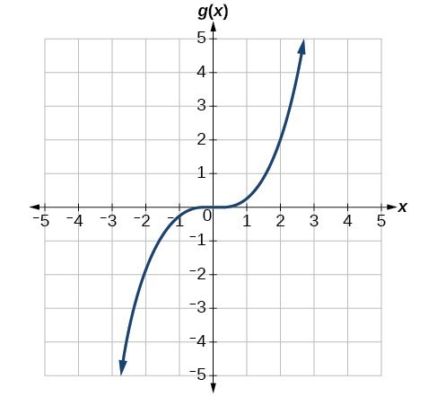
Figure 17
The graph is a transformation of the toolkit function [latex]f\left(x\right)={x}^{3}\\[/latex]. Relate this new function [latex]g\left(x\right)\\[/latex] to [latex]f\left(x\right)\\[/latex], and then find a formula for [latex]g\left(x\right)\\[/latex].
When trying to determine a vertical stretch or shift, it is helpful to look for a point on the graph that is relatively clear. In this graph, it appears that [latex]g\left(2\right)=2\\[/latex]. With the basic cubic function at the same input, [latex]f\left(2\right)={2}^{3}=8\\[/latex]. Based on that, it appears that the outputs of [latex]g\\[/latex] are [latex]\frac{1}{4}\\[/latex] the outputs of the function [latex]f\\[/latex] because [latex]g\left(2\right)=\frac{1}{4}f\left(2\right)\\[/latex]. From this we can fairly safely conclude that [latex]g\left(x\right)=\frac{1}{4}f\left(x\right)\\[/latex].
We can write a formula for [latex]g\\[/latex] by using the definition of the function [latex]f\\[/latex].
Write the formula for the function that we get when we stretch the identity toolkit function by a factor of 3, and then shift it down by 2 units.
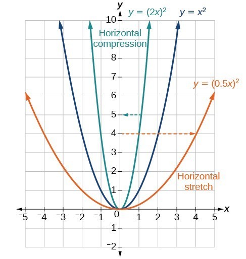
Figure 18
Now we consider changes to the inside of a function. When we multiply a function’s input by a positive constant, we get a function whose graph is stretched or compressed horizontally in relation to the graph of the original function. If the constant is between 0 and 1, we get a horizontal stretch; if the constant is greater than 1, we get a horizontal compression of the function.
Given a function [latex]y=f\left(x\right)\\[/latex], the form [latex]y=f\left(bx\right)[/latex] results in a horizontal stretch or compression. Consider the function [latex]y={x}^{2}\\[/latex]. The graph of [latex]y={\left(0.5x\right)}^{2}\\[/latex] is a horizontal stretch of the graph of the function [latex]y={x}^{2}\\[/latex] by a factor of 2. The graph of [latex]y={\left(2x\right)}^{2}\\[/latex] is a horizontal compression of the graph of the function [latex]y={x}^{2}\\[/latex] by a factor of 2.
Given a function [latex]f\left(x\right)\\[/latex], a new function [latex]g\left(x\right)=f\left(bx\right)\\[/latex], where [latex]b\\[/latex] is a constant, is a horizontal stretch or horizontal compression of the function [latex]f\left(x\right)\\[/latex].
Suppose a scientist is comparing a population of fruit flies to a population that progresses through its lifespan twice as fast as the original population. In other words, this new population, [latex]R\\[/latex], will progress in 1 hour the same amount as the original population does in 2 hours, and in 2 hours, it will progress as much as the original population does in 4 hours. Sketch a graph of this population.
Symbolically, we could write
See below for a graphical comparison of the original population and the compressed population.
![Two side-by-side graphs. The first graph has function for original population whose domain is [0,7] and range is [0,3]. The maximum value occurs at (3,3). The second graph has the same shape as the first except it is half as wide. It is a graph of transformed population, with a domain of [0, 3.5] and a range of [0,3]. The maximum occurs at (1.5, 3).](https://s3-us-west-2.amazonaws.com/courses-images-archive-read-only/wp-content/uploads/sites/924/2015/11/25200820/CNX_Precalc_Figure_01_05_029ab.jpg)
Figure 19. (a) Original population graph (b) Compressed population graph
Note that the effect on the graph is a horizontal compression where all input values are half of their original distance from the vertical axis.
A function [latex]f\left(x\right)\\[/latex] is given below. Create a table for the function [latex]g\left(x\right)=f\left(\frac{1}{2}x\right)\\[/latex].
| [latex]x[/latex] | 2 | 4 | 6 | 8 |
| [latex]f\left(x\right)[/latex] | 1 | 3 | 7 | 11 |
The formula [latex]g\left(x\right)=f\left(\frac{1}{2}x\right)\\[/latex] tells us that the output values for [latex]g\\[/latex] are the same as the output values for the function [latex]f\\[/latex] at an input half the size. Notice that we do not have enough information to determine [latex]g\left(2\right)\\[/latex] because [latex]g\left(2\right)=f\left(\frac{1}{2}\cdot 2\right)=f\left(1\right)\\[/latex], and we do not have a value for [latex]f\left(1\right)\\[/latex] in our table. Our input values to [latex]g\\[/latex] will need to be twice as large to get inputs for [latex]f\\[/latex] that we can evaluate. For example, we can determine [latex]g\left(4\right)\text{.}\\[/latex]
We do the same for the other values to produce the table below.
| [latex]x[/latex] | 4 | 8 | 12 | 16 |
| [latex]g\left(x\right)[/latex] | 1 | 3 | 7 | 11 |
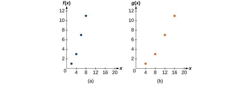
Figure 20
This figure shows the graphs of both of these sets of points.
Because each input value has been doubled, the result is that the function [latex]g\left(x\right)\\[/latex] has been stretched horizontally by a factor of 2.
Relate the function [latex]g\left(x\right)\\[/latex] to [latex]f\left(x\right)\\[/latex] in Figure 21.
Figure 21
The graph of [latex]g\left(x\right)\\[/latex] looks like the graph of [latex]f\left(x\right)\\[/latex] horizontally compressed. Because [latex]f\left(x\right)\\[/latex] ends at [latex]\left(6,4\right)\\[/latex] and [latex]g\left(x\right)\\[/latex] ends at [latex]\left(2,4\right)\\[/latex], we can see that the [latex]x\text{-}\\[/latex] values have been compressed by [latex]\frac{1}{3}\\[/latex], because [latex]6\left(\frac{1}{3}\right)=2\\[/latex]. We might also notice that [latex]g\left(2\right)=f\left(6\right)\\[/latex] and [latex]g\left(1\right)=f\left(3\right)\\[/latex]. Either way, we can describe this relationship as [latex]g\left(x\right)=f\left(3x\right)\\[/latex]. This is a horizontal compression by [latex]\frac{1}{3}\\[/latex].
Notice that the coefficient needed for a horizontal stretch or compression is the reciprocal of the stretch or compression. So to stretch the graph horizontally by a scale factor of 4, we need a coefficient of [latex]\frac{1}{4}\\[/latex] in our function: [latex]f\left(\frac{1}{4}x\right)\\[/latex]. This means that the input values must be four times larger to produce the same result, requiring the input to be larger, causing the horizontal stretching.
Write a formula for the toolkit square root function horizontally stretched by a factor of 3.
Now that we have two transformations, we can combine them together. Vertical shifts are outside changes that affect the output ( [latex]y\text{-}\\[/latex] ) axis values and shift the function up or down. Horizontal shifts are inside changes that affect the input ( [latex]x\text{-}\\[/latex] ) axis values and shift the function left or right. Combining the two types of shifts will cause the graph of a function to shift up or down and right or left.
Given [latex]f\left(x\right)=|x|\\[/latex], sketch a graph of [latex]h\left(x\right)=f\left(x+1\right)-3\\[/latex].
The function [latex]f\\[/latex] is our toolkit absolute value function. We know that this graph has a V shape, with the point at the origin. The graph of [latex]h\\[/latex] has transformed [latex]f\\[/latex] in two ways: [latex]f\left(x+1\right)\\[/latex] is a change on the inside of the function, giving a horizontal shift left by 1, and the subtraction by 3 in [latex]f\left(x+1\right)-3\\[/latex] is a change to the outside of the function, giving a vertical shift down by 3. The transformation of the graph is illustrated in Figure 22.
Let us follow one point of the graph of [latex]f\left(x\right)=|x|\\[/latex].

Figure 22
Figure 23 is the graph of [latex]h\\[/latex].
Figure 23
Given [latex]f\left(x\right)=|x|\\[/latex], sketch a graph of [latex]h\left(x\right)=f\left(x - 2\right)+4\\[/latex].
Write a formula for the graph shown in Figure 24, which is a transformation of the toolkit square root function.
Figure 24
The graph of the toolkit function starts at the origin, so this graph has been shifted 1 to the right and up 2. In function notation, we could write that as
Using the formula for the square root function, we can write
Note that this transformation has changed the domain and range of the function. This new graph has domain [latex]\left[1,\infty \right)\\[/latex] and range [latex]\left[2,\infty \right)\\[/latex].
Write a formula for a transformation of the toolkit reciprocal function [latex]f\left(x\right)=\frac{1}{x}\\[/latex] that shifts the function’s graph one unit to the right and one unit up.
A common model for learning has an equation similar to [latex]k\left(t\right)=-{2}^{-t}+1\\[/latex], where [latex]k\\[/latex] is the percentage of mastery that can be achieved after [latex]t\\[/latex] practice sessions. This is a transformation of the function [latex]f\left(t\right)={2}^{t}\\[/latex] shown in Figure 25. Sketch a graph of [latex]k\left(t\right)\\[/latex].
Figure 25
This equation combines three transformations into one equation.
We can sketch a graph by applying these transformations one at a time to the original function. Let us follow two points through each of the three transformations. We will choose the points (0, 1) and (1, 2).
This means that the original points, (0,1) and (1,2) become (0,0) and (1,1) after we apply the transformations.
In Figure 26, the first graph results from a horizontal reflection. The second results from a vertical reflection. The third results from a vertical shift up 1 unit.
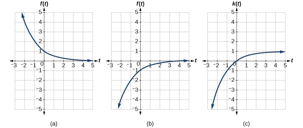
Figure 26
As a model for learning, this function would be limited to a domain of [latex]t\ge 0\\[/latex], with corresponding range [latex]\left[0,1\right)\\[/latex].
Given the toolkit function [latex]f\left(x\right)={x}^{2}\\[/latex], graph [latex]g\left(x\right)=-f\left(x\right)\\[/latex] and [latex]h\left(x\right)=f\left(-x\right)\\[/latex]. Take note of any surprising behavior for these functions.
When combining transformations, it is very important to consider the order of the transformations. For example, vertically shifting by 3 and then vertically stretching by 2 does not create the same graph as vertically stretching by 2 and then vertically shifting by 3, because when we shift first, both the original function and the shift get stretched, while only the original function gets stretched when we stretch first.
When we see an expression such as [latex]2f\left(x\right)+3\\[/latex], which transformation should we start with? The answer here follows nicely from the order of operations. Given the output value of [latex]f\left(x\right)\\[/latex], we first multiply by 2, causing the vertical stretch, and then add 3, causing the vertical shift. In other words, multiplication before addition.
Horizontal transformations are a little trickier to think about. When we write [latex]g\left(x\right)=f\left(2x+3\right)\\[/latex], for example, we have to think about how the inputs to the function [latex]g[/latex] relate to the inputs to the function [latex]f\\[/latex]. Suppose we know [latex]f\left(7\right)=12\\[/latex]. What input to [latex]g\\[/latex] would produce that output? In other words, what value of [latex]x\\[/latex] will allow [latex]g\left(x\right)=f\left(2x+3\right)=12?\\[/latex] We would need [latex]2x+3=7\\[/latex]. To solve for [latex]x\\[/latex], we would first subtract 3, resulting in a horizontal shift, and then divide by 2, causing a horizontal compression.
This format ends up being very difficult to work with, because it is usually much easier to horizontally stretch a graph before shifting. We can work around this by factoring inside the function.
Let’s work through an example.
We can factor out a 2.
Now we can more clearly observe a horizontal shift to the left 2 units and a horizontal compression. Factoring in this way allows us to horizontally stretch first and then shift horizontally.
When combining vertical transformations written in the form [latex]af\left(x\right)+k\\[/latex], first vertically stretch by [latex]a\\[/latex] and then vertically shift by [latex]k\\[/latex].
When combining horizontal transformations written in the form [latex]f\left(bx+h\right)\\[/latex], first horizontally shift by [latex]h[/latex] and then horizontally stretch by [latex]\frac{1}{b}\\[/latex].
When combining horizontal transformations written in the form [latex]f\left(b\left(x+h\right)\right)\\[/latex], first horizontally stretch by [latex]\frac{1}{b}[/latex] and then horizontally shift by [latex]h\\[/latex].
Horizontal and vertical transformations are independent. It does not matter whether horizontal or vertical transformations are performed first.
Given the table below for the function [latex]f\left(x\right)\\[/latex], create a table of values for the function [latex]g\left(x\right)=2f\left(3x\right)+1\\[/latex].
| [latex]x[/latex] | 6 | 12 | 18 | 24 |
| [latex]f\left(x\right)[/latex] | 10 | 14 | 15 | 17 |
There are three steps to this transformation, and we will work from the inside out. Starting with the horizontal transformations, [latex]f\left(3x\right)[/latex] is a horizontal compression by [latex]\frac{1}{3}\\[/latex], which means we multiply each [latex]x\text{-}\\[/latex] value by [latex]\frac{1}{3}\\[/latex].
| [latex]x[/latex] | 2 | 4 | 6 | 8 |
| [latex]f\left(3x\right)[/latex] | 10 | 14 | 15 | 17 |
Looking now to the vertical transformations, we start with the vertical stretch, which will multiply the output values by 2. We apply this to the previous transformation.
| [latex]x\\[/latex] | 2 | 4 | 6 | 8 |
| [latex]2f\left(3x\right)\\[/latex] | 20 | 28 | 30 | 34 |
Finally, we can apply the vertical shift, which will add 1 to all the output values.
| [latex]x\\[/latex] | 2 | 4 | 6 | 8 |
| [latex]g\left(x\right)=2f\left(3x\right)+1\\[/latex] | 21 | 29 | 31 | 35 |
Use the graph of [latex]f\left(x\right)\\[/latex] to sketch a graph of [latex]k\left(x\right)=f\left(\frac{1}{2}x+1\right)-3\\[/latex].
Figure 27
To simplify, let’s start by factoring out the inside of the function.
[latex]f\left(\frac{1}{2}x+1\right)-3=f\left(\frac{1}{2}\left(x+2\right)\right)-3\\[/latex]
Figure 28
Next, we horizontally shift left by 2 units, as indicated by [latex]x+2\\[/latex].
Figure 29
Last, we vertically shift down by 3 to complete our sketch, as indicated by the [latex]-3\\[/latex] on the outside of the function.
Figure 30
| Vertical shift | [latex]g\left(x\right)=f\left(x\right)+k\\[/latex] (up for [latex]k>0\\[/latex] ) |
| Horizontal shift | [latex]g\left(x\right)=f\left(x-h\right)\\[/latex] (right for [latex]h>0\\[/latex] ) |
| Vertical reflection | [latex]g\left(x\right)=-f\left(x\right)\\[/latex] |
| Horizontal reflection | [latex]g\left(x\right)=f\left(-x\right)\\[/latex] |
| Vertical stretch | [latex]g\left(x\right)=af\left(x\right)\\[/latex] ( [latex]a>0\\[/latex]) |
| Vertical compression | [latex]g\left(x\right)=af\left(x\right)\\[/latex] [latex]\left(0<a<1\right)\\[/latex] |
| Horizontal stretch | [latex]g\left(x\right)=f\left(bx\right)\\[/latex] [latex]\left(0<b<1\right)\\[/latex] |
| Horizontal compression | [latex]g\left(x\right)=f\left(bx\right)\\[/latex] ( [latex]b>1\\[/latex] ) |
1. When examining the formula of a function that is the result of multiple transformations, how can you tell a horizontal shift from a vertical shift?
2. When examining the formula of a function that is the result of multiple transformations, how can you tell a horizontal stretch from a vertical stretch?
3. When examining the formula of a function that is the result of multiple transformations, how can you tell a horizontal compression from a vertical compression?
4. When examining the formula of a function that is the result of multiple transformations, how can you tell a reflection with respect to the x-axis from a reflection with respect to the y-axis?
5. How can you determine whether a function is odd or even from the formula of the function?
6. Write a formula for the function obtained when the graph of [latex]f\left(x\right)=\sqrt{x}\\[/latex] is shifted up 1 unit and to the left 2 units.
7. Write a formula for the function obtained when the graph of [latex]f\left(x\right)=|x|\\[/latex]
is shifted down 3 units and to the right 1 unit.
8. Write a formula for the function obtained when the graph of [latex]f\left(x\right)=\frac{1}{x}\\[/latex] is shifted down 4 units and to the right 3 units.
9. Write a formula for the function obtained when the graph of [latex]f\left(x\right)=\frac{1}{{x}^{2}}\\[/latex] is shifted up 2 units and to the left 4 units.
For the following exercises, describe how the graph of the function is a transformation of the graph of the original function [latex]f\\[/latex].
10. [latex]y=f\left(x - 49\right)\\[/latex]
11. [latex]y=f\left(x+43\right)\\[/latex]
12. [latex]y=f\left(x+3\right)\\[/latex]
13. [latex]y=f\left(x - 4\right)\\[/latex]
14. [latex]y=f\left(x\right)+5\\[/latex]
15. [latex]y=f\left(x\right)+8\\[/latex]
16. [latex]y=f\left(x\right)-2\\[/latex]
17. [latex]y=f\left(x\right)-7\\[/latex]
18. [latex]y=f\left(x - 2\right)+3\\[/latex]
19. [latex]y=f\left(x+4\right)-1\\[/latex]
For the following exercises, determine the interval(s) on which the function is increasing and decreasing.
20. [latex]f\left(x\right)=4{\left(x+1\right)}^{2}-5\\[/latex]
21. [latex]g\left(x\right)=5{\left(x+3\right)}^{2}-2\\[/latex]
22. [latex]a\left(x\right)=\sqrt{-x+4}\\[/latex]
23. [latex]k\left(x\right)=-3\sqrt{x}-1\\[/latex]
For the following exercises, use the graph of [latex]f\left(x\right)={2}^{x}\\[/latex] to sketch a graph of each transformation of [latex]f\left(x\right)\\[/latex].
24. [latex]g\left(x\right)={2}^{x}+1\\[/latex]
25. [latex]h\left(x\right)={2}^{x}-3\\[/latex]
26. [latex]w\left(x\right)={2}^{x - 1}\\[/latex]
For the following exercises, sketch a graph of the function as a transformation of the graph of one of the toolkit functions.
27. [latex]f\left(t\right)={\left(t+1\right)}^{2}-3\\[/latex]
28. [latex]h\left(x\right)=|x - 1|+4\\[/latex]
29. [latex]k\left(x\right)={\left(x - 2\right)}^{3}-1\\[/latex]
30. [latex]m\left(t\right)=3+\sqrt{t+2}\\[/latex]
31. Tabular representations for the functions [latex]f,g\\[/latex], and [latex]h[/latex] are given below. Write [latex]g\left(x\right)\\[/latex] and [latex]h\left(x\right)\\[/latex] as transformations of [latex]f\left(x\right)\\[/latex].
| [latex]x\\[/latex] | −2 | −1 | 0 | 1 | 2 |
| [latex]f\left(x\right)\\[/latex] | −2 | −1 | −3 | 1 | 2 |
| [latex]x\\[/latex] | −1 | 0 | 1 | 2 | 3 |
| [latex]g\left(x\right)\\[/latex] | −2 | −1 | −3 | 1 | 2 |
| [latex]x\\[/latex] | −2 | −1 | 0 | 1 | 2 |
| [latex]h\left(x\right)\\[/latex] | −1 | 0 | −2 | 2 | 3 |
32. Tabular representations for the functions [latex]f,g\\[/latex], and [latex]h\\[/latex] are given below. Write [latex]g\left(x\right)\\[/latex] and [latex]h\left(x\right)\\[/latex] as transformations of [latex]f\left(x\right)\\[/latex].
| [latex]x\\[/latex] | −2 | −1 | 0 | 1 | 2 |
| [latex]f\left(x\right)\\[/latex] | −1 | −3 | 4 | 2 | 1 |
| [latex]x\\[/latex] | −3 | −2 | −1 | 0 | 1 |
| [latex]g\left(x\right)\\[/latex] | −1 | −3 | 4 | 2 | 1 |
| [latex]x\\[/latex] | −2 | −1 | 0 | 1 | 2 |
| [latex]h\left(x\right)\\[/latex] | −2 | −4 | 3 | 1 | 0 |
For the following exercises, write an equation for each graphed function by using transformations of the graphs of one of the toolkit functions.
33.

34.
35.
36.
37.
38.
39.
40.
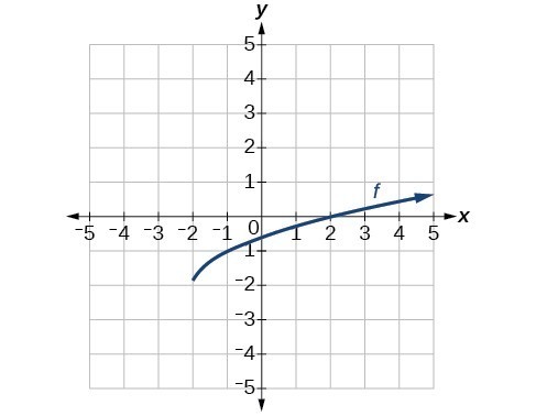
For the following exercises, use the graphs of transformations of the square root function to find a formula for each of the functions.
41.
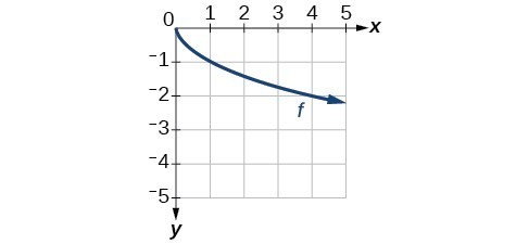
42.
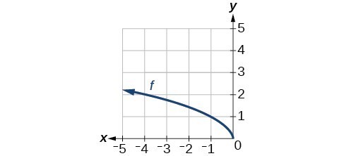
For the following exercises, use the graphs of the transformed toolkit functions to write a formula for each of the resulting functions.
43.
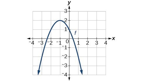
44.
45.
46.
For the following exercises, determine whether the function is odd, even, or neither.
47. [latex]f\left(x\right)=3{x}^{4}\\[/latex]
48. [latex]g\left(x\right)=\sqrt{x}\\[/latex]
49. [latex]h\left(x\right)=\frac{1}{x}+3x\\[/latex]
50. [latex]f\left(x\right)={\left(x - 2\right)}^{2}\\[/latex]
51. [latex]g\left(x\right)=2{x}^{4}\\[/latex]
52. [latex]h\left(x\right)=2x-{x}^{3}\\[/latex]
For the following exercises, describe how the graph of each function is a transformation of the graph of the original function [latex]f[/latex].
53. [latex]g\left(x\right)=-f\left(x\right)\\[/latex]
54. [latex]g\left(x\right)=f\left(-x\right)\\[/latex]
55. [latex]g\left(x\right)=4f\left(x\right)\\[/latex]
56. [latex]g\left(x\right)=6f\left(x\right)\\[/latex]
57. [latex]g\left(x\right)=f\left(5x\right)\\[/latex]
58. [latex]g\left(x\right)=f\left(2x\right)\\[/latex]
59. [latex]g\left(x\right)=f\left(\frac{1}{3}x\right)\\[/latex]
60. [latex]g\left(x\right)=f\left(\frac{1}{5}x\right)\\[/latex]
61. [latex]g\left(x\right)=3f\left(-x\right)\\[/latex]
62. [latex]g\left(x\right)=-f\left(3x\right)\\[/latex]
For the following exercises, write a formula for the function [latex]g\\[/latex] that results when the graph of a given toolkit function is transformed as described.
63. The graph of [latex]f\left(x\right)=|x|\\[/latex] is reflected over the [latex]y\\[/latex] –axis and horizontally compressed by a factor of [latex]\frac{1}{4}\\[/latex] .
64. The graph of [latex]f\left(x\right)=\sqrt{x}\\[/latex] is reflected over the [latex]x\\[/latex] -axis and horizontally stretched by a factor of 2.
65. The graph of [latex]f\left(x\right)=\frac{1}{{x}^{2}}\\[/latex] is vertically compressed by a factor of [latex]\frac{1}{3}\\[/latex], then shifted to the left 2 units and down 3 units.
66. The graph of [latex]f\left(x\right)=\frac{1}{x}\\[/latex] is vertically stretched by a factor of 8, then shifted to the right 4 units and up 2 units.
67. The graph of [latex]f\left(x\right)={x}^{2}\\[/latex] is vertically compressed by a factor of [latex]\frac{1}{2}\\[/latex], then shifted to the right 5 units and up 1 unit.
68. The graph of [latex]f\left(x\right)={x}^{2}\\[/latex] is horizontally stretched by a factor of 3, then shifted to the left 4 units and down 3 units.
For the following exercises, describe how the formula is a transformation of a toolkit function. Then sketch a graph of the transformation.
69. [latex]g\left(x\right)=4{\left(x+1\right)}^{2}-5\\[/latex]
70. [latex]g\left(x\right)=5{\left(x+3\right)}^{2}-2\\[/latex]
71. [latex]h\left(x\right)=-2|x - 4|+3\\[/latex]
72. [latex]k\left(x\right)=-3\sqrt{x}-1\\[/latex]
73. [latex]m\left(x\right)=\frac{1}{2}{x}^{3}\\[/latex]
74. [latex]n\left(x\right)=\frac{1}{3}|x - 2|\\[/latex]
75. [latex]p\left(x\right)={\left(\frac{1}{3}x\right)}^{3}-3\\[/latex]
76. [latex]q\left(x\right)={\left(\frac{1}{4}x\right)}^{3}+1\\[/latex]
77. [latex]a\left(x\right)=\sqrt{-x+4}\\[/latex]
For the following exercises, use the graph below to sketch the given transformations.
78. [latex]g\left(x\right)=f\left(x\right)-2\\[/latex]
79. [latex]g\left(x\right)=-f\left(x\right)\\[/latex]
80. [latex]g\left(x\right)=f\left(x+1\right)\\[/latex]
81. [latex]g\left(x\right)=f\left(x - 2\right)\\[/latex]
1. The graphs of [latex]f\left(x\right)\\[/latex] and [latex]g\left(x\right)\\[/latex] are shown below. The transformation is a horizontal shift. The function is shifted to the left by 2 units.
2.
a)
b)
3. [latex]g\left(x\right)=-f\left(x\right)\\[/latex]
| [latex]x\\[/latex] | -2 | 0 | 2 | 4 |
| [latex]g\left(x\right)\\[/latex] | [latex]-5\\[/latex] | [latex]-10\\[/latex] | [latex]-15\\[/latex] | [latex]-20\\[/latex] |
[latex]h\left(x\right)=f\left(-x\right)\\[/latex]
| [latex]x\\[/latex] | -2 | 0 | 2 | 4 |
| [latex]h\left(x\right)\\[/latex] | 15 | 10 | 5 | unknown |
4. even
5.
| [latex]x\\[/latex] | 2 | 4 | 6 | 8 |
| [latex]g\left(x\right)\\[/latex] | 9 | 12 | 15 | 0 |
6. [latex]g\left(x\right)=3x - 2\\[/latex]
7. [latex]g\left(x\right)=f\left(\frac{1}{3}x\right)\\[/latex] so using the square root function we get [latex]g\left(x\right)=\sqrt{\frac{1}{3}x}\\[/latex]
8.
9. [latex]g\left(x\right)=\frac{1}{x - 1}+1\\[/latex]
10. Notice: [latex]g\left(x\right)=f\left(-x\right)\\[/latex] looks the same as [latex]f\left(x\right)\\[/latex] .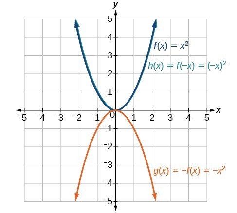
1. A horizontal shift results when a constant is added to or subtracted from the input. A vertical shifts results when a constant is added to or subtracted from the output.
3. A horizontal compression results when a constant greater than 1 is multiplied by the input. A vertical compression results when a constant between 0 and 1 is multiplied by the output.
5. For a function [latex]f[/latex], substitute [latex]\left(-x\right)\\[/latex] for [latex]\left(x\right)\\[/latex] in [latex]f\left(x\right)\\[/latex]. Simplify. If the resulting function is the same as the original function, [latex]f\left(-x\right)=f\left(x\right)\\[/latex], then the function is even. If the resulting function is the opposite of the original function, [latex]f\left(-x\right)=-f\left(x\right)\\[/latex], then the original function is odd. If the function is not the same or the opposite, then the function is neither odd nor even.
7. [latex]g\left(x\right)=|x - 1|-3\\[/latex]
9. [latex]g\left(x\right)=\frac{1}{{\left(x+4\right)}^{2}}+2\\[/latex]
11. The graph of [latex]f\left(x+43\right)\\[/latex] is a horizontal shift to the left 43 units of the graph of [latex]f\\[/latex].
13. The graph of [latex]f\left(x - 4\right)\\[/latex] is a horizontal shift to the right 4 units of the graph of [latex]f\\[/latex].
15. The graph of [latex]f\left(x\right)+8\\[/latex] is a vertical shift up 8 units of the graph of [latex]f\\[/latex].
17. The graph of [latex]f\left(x\right)-7\\[/latex] is a vertical shift down 7 units of the graph of [latex]f\\[/latex].
19. The graph of [latex]f\left(x+4\right)-1\\[/latex] is a horizontal shift to the left 4 units and a vertical shift down 1 unit of the graph of [latex]f\\[/latex].
21. decreasing on [latex]\left(-\infty ,-3\right)\\[/latex] and increasing on [latex]\left(-3,\infty \right)\\[/latex]
23. decreasing on [latex]\left(0,\infty \right)\\[/latex]
25.
27.
29.
31. [latex]g\left(x\right)=f\left(x - 1\right),h\left(x\right)=f\left(x\right)+1\\[/latex]
33. [latex]f\left(x\right)=|x - 3|-2\\[/latex]
35. [latex]f\left(x\right)=\sqrt{x+3}-1\\[/latex]
37. [latex]f\left(x\right)={\left(x - 2\right)}^{2}\\[/latex]
39. [latex]f\left(x\right)=|x+3|-2\\[/latex]
41. [latex]f\left(x\right)=-\sqrt{x}\\[/latex]
43. [latex]f\left(x\right)=-{\left(x+1\right)}^{2}+2\\[/latex]
45. [latex]f\left(x\right)=\sqrt{-x}+1\\[/latex]
47. even
49. odd
51. even
53. The graph of [latex]g\\[/latex] is a vertical reflection (across the [latex]x\\[/latex] -axis) of the graph of [latex]f\\[/latex].
55. The graph of [latex]g\\[/latex] is a vertical stretch by a factor of 4 of the graph of [latex]f\\[/latex].
57. The graph of [latex]g\\[/latex] is a horizontal compression by a factor of [latex]\frac{1}{5}\\[/latex] of the graph of [latex]f\\[/latex].
59. The graph of [latex]g\\[/latex] is a horizontal stretch by a factor of 3 of the graph of [latex]f\\[/latex].
61. The graph of [latex]g\\[/latex] is a horizontal reflection across the [latex]y\\[/latex] -axis and a vertical stretch by a factor of 3 of the graph of [latex]f\\[/latex].
63. [latex]g\left(x\right)=|-4x|\\[/latex]
65. [latex]g\left(x\right)=\frac{1}{3{\left(x+2\right)}^{2}}-3\\[/latex]
67. [latex]g\left(x\right)=\frac{1}{2}{\left(x - 5\right)}^{2}+1\\[/latex]
69. The graph of the function [latex]f\left(x\right)={x}^{2}\\[/latex] is shifted to the left 1 unit, stretched vertically by a factor of 4, and shifted down 5 units.
71. The graph of [latex]f\left(x\right)=|x|\\[/latex] is stretched vertically by a factor of 2, shifted horizontally 4 units to the right, reflected across the horizontal axis, and then shifted vertically 3 units up.
73. The graph of the function [latex]f\left(x\right)={x}^{3}\\[/latex] is compressed vertically by a factor of [latex]\frac{1}{2}\\[/latex].
75. The graph of the function is stretched horizontally by a factor of 3 and then shifted vertically downward by 3 units.
77. The graph of [latex]f\left(x\right)=\sqrt{x}\\[/latex] is shifted right 4 units and then reflected across the vertical line [latex]x=4\\[/latex].
79.
81.
By the end of this lesson, you will be able to:

Figure 1. Distances in deep space can be measured in all directions. As such, it is useful to consider distance in terms of absolute values. (credit: “s58y”/Flickr)
Until the 1920s, the so-called spiral nebulae were believed to be clouds of dust and gas in our own galaxy, some tens of thousands of light years away. Then, astronomer Edwin Hubble proved that these objects are galaxies in their own right, at distances of millions of light years. Today, astronomers can detect galaxies that are billions of light years away. Distances in the universe can be measured in all directions. As such, it is useful to consider distance as an absolute value function. In this section, we will investigate absolute value functions.
Recall that in its basic form [latex]\displaystyle{f}\left({x}\right)={|x|}\\[/latex], the absolute value function, is one of our toolkit functions. The absolute value function is commonly thought of as providing the distance the number is from zero on a number line. Algebraically, for whatever the input value is, the output is the value without regard to sign.
The absolute value function can be defined as a piecewise function
[latex]f(x) = \begin{cases} x ,\ x \geq 0 \\ -x , x < 0\\ \end{cases} [/latex]
Describe all values [latex]x\\[/latex] within or including a distance of 4 from the number 5.
Figure 2
We want the distance between [latex]x\\[/latex] and 5 to be less than or equal to 4. We can draw a number line to represent the condition to be satisfied.
The distance from [latex]x\\[/latex] to 5 can be represented using the absolute value as [latex]|x - 5|\\[/latex]. We want the values of [latex]x\\[/latex] that satisfy the condition [latex]|x - 5|\le 4\\[/latex].
Note that
So [latex]|x - 5|\le 4\\[/latex] is equivalent to [latex]1\le x\le 9\\[/latex].
However, mathematicians generally prefer absolute value notation.
Electrical parts, such as resistors and capacitors, come with specified values of their operating parameters: resistance, capacitance, etc. However, due to imprecision in manufacturing, the actual values of these parameters vary somewhat from piece to piece, even when they are supposed to be the same. The best that manufacturers can do is to try to guarantee that the variations will stay within a specified range, often [latex]\displaystyle\text{\pm 1%,}\pm\text{5%,}\\[/latex] or [latex]\displaystyle\pm\text{10%}\\[/latex].
Suppose we have a resistor rated at 680 ohms, [latex]\pm 5%\\[/latex]. Use the absolute value function to express the range of possible values of the actual resistance.
5% of 680 ohms is 34 ohms. The absolute value of the difference between the actual and nominal resistance should not exceed the stated variability, so, with the resistance [latex]R\\[/latex] in ohms,
Students who score within 20 points of 80 will pass a test. Write this as a distance from 80 using absolute value notation.
The most significant feature of the absolute value graph is the corner point at which the graph changes direction. This point is shown at the origin.
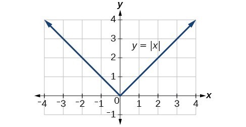
Figure 3
Figure 4 is the graph of [latex]y=2\left|x - 3\right|+4\\[/latex]. The graph of [latex]y=|x|\\[/latex] has been shifted right 3 units, vertically stretched by a factor of 2, and shifted up 4 units. This means that the corner point is located at [latex]\left(3,4\right)\\[/latex] for this transformed function.
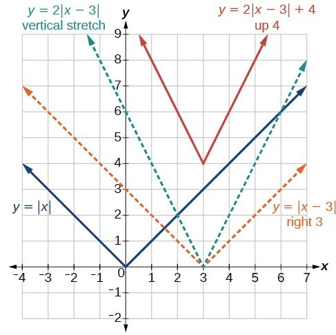
Figure 4
Write an equation for the function graphed in Figure 5.
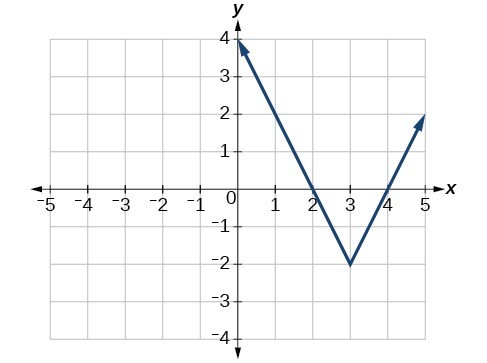
Figure 5
The basic absolute value function changes direction at the origin, so this graph has been shifted to the right 3 units and down 2 units from the basic toolkit function.
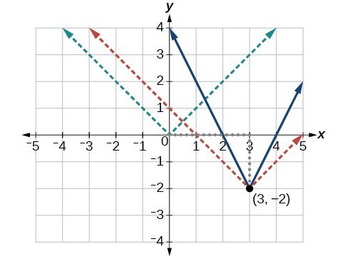
Figure 6
We also notice that the graph appears vertically stretched, because the width of the final graph on a horizontal line is not equal to 2 times the vertical distance from the corner to this line, as it would be for an unstretched absolute value function. Instead, the width is equal to 1 times the vertical distance.
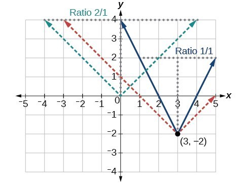
Figure 7
From this information we can write the equation
Note that these equations are algebraically equivalent—the stretch for an absolute value function can be written interchangeably as a vertical or horizontal stretch or compression.
Q & A
If we couldn’t observe the stretch of the function from the graphs, could we algebraically determine it?
Yes. If we are unable to determine the stretch based on the width of the graph, we can solve for the stretch factor by putting in a known pair of values for [latex]x\\[/latex] and [latex]f\left(x\right)\\[/latex].
Now substituting in the point (1, 2)
Write the equation for the absolute value function that is horizontally shifted left 2 units, is vertically flipped, and vertically shifted up 3 units.
Q & A
Do the graphs of absolute value functions always intersect the vertical axis? The horizontal axis?
Yes, they always intersect the vertical axis. The graph of an absolute value function will intersect the vertical axis when the input is zero.
No, they do not always intersect the horizontal axis. The graph may or may not intersect the horizontal axis, depending on how the graph has been shifted and reflected. It is possible for the absolute value function to intersect the horizontal axis at zero, one, or two points.
Figure 8. (a) The absolute value function does not intersect the horizontal axis. (b) The absolute value function intersects the horizontal axis at one point. (c) The absolute value function intersects the horizontal axis at two points.
Now that we can graph an absolute value function, we will learn how to solve an absolute value equation. To solve an equation such as [latex]{8}=\left|{2}x - {6}\right|\\[/latex], we notice that the absolute value will be equal to 8 if the quantity inside the absolute value is 8 or -8. This leads to two different equations we can solve independently.
Knowing how to solve problems involving absolute value functions is useful. For example, we may need to identify numbers or points on a line that are at a specified distance from a given reference point.
An absolute value equation is an equation in which the unknown variable appears in absolute value bars. For example,
For real numbers [latex]A\\[/latex] and [latex]B\\[/latex], an equation of the form [latex]|A|=B\\[/latex], with [latex]B\ge 0\\[/latex], will have solutions when [latex]A=B\\[/latex] or [latex]A=-B\\[/latex]. If [latex]B<0\\[/latex], the equation [latex]|A|=B\\[/latex] has no solution.
For the function [latex]f\left(x\right)=|4x+1|-7\\[/latex] , find the values of [latex]x\\[/latex] such that [latex]\text{ }f\left(x\right)=0\\[/latex] .
[latex]\begin{cases}0=|4x+1|-7\hfill & \hfill & \hfill & \hfill & \hfill & \hfill & \text{Substitute 0 for }f\left(x\right).\hfill \\ 7=|4x+1|\hfill & \hfill & \hfill & \hfill & \hfill & \hfill & \text{Isolate the absolute value on one side of the equation}.\hfill \\ \hfill & \hfill & \hfill & \hfill & \hfill & \hfill & \hfill \\ \hfill & \hfill & \hfill & \hfill & \hfill & \hfill & \hfill \\ \hfill & \hfill & \hfill & \hfill & \hfill & \hfill & \hfill \\ 7=4x+1\hfill & \text{or}\hfill & \hfill & \hfill & \hfill & -7=4x+1\hfill & \text{Break into two separate equations and solve}.\hfill \\ 6=4x\hfill & \hfill & \hfill & \hfill & \hfill & -8=4x\hfill & \hfill \\ \hfill & \hfill & \hfill & \hfill & \hfill & \hfill & \hfill \\ x=\frac{6}{4}=1.5\hfill & \hfill & \hfill & \hfill & \hfill & \text{ }x=\frac{-8}{4}=-2\hfill & \hfill \end{cases}\\[/latex]
Figure 9
The function outputs 0 when [latex]x=1.5[/latex] or [latex]x=-2\\[/latex].
For the function [latex]f\left(x\right)=|2x - 1|-3\\[/latex], find the values of [latex]x\\[/latex] such that [latex]f\left(x\right)=0\\[/latex].
Q & A
Should we always expect two answers when solving [latex]|A|=B?\\[/latex]
No. We may find one, two, or even no answers. For example, there is no solution to [latex]2+|3x - 5|=1\\[/latex].
Solve [latex]1=4|x - 2|+2\\[/latex].
Isolating the absolute value on one side of the equation gives the following.
The absolute value always returns a positive value, so it is impossible for the absolute value to equal a negative value. At this point, we notice that this equation has no solutions.
Q & A
In Example 5, if [latex]f\left(x\right)=1\\[/latex] and [latex]g\left(x\right)=4|x - 2|+2\\[/latex] were graphed on the same set of axes, would the graphs intersect?
No. The graphs of [latex]f\\[/latex] and [latex]g\\[/latex] would not intersect. This confirms, graphically, that the equation [latex]1=4|x - 2|+2\\[/latex] has no solution.
Figure 10
Find where the graph of the function [latex]f\left(x\right)=-|x+2|+3\\[/latex] intersects the horizontal and vertical axes.
Absolute value equations may not always involve equalities. Instead, we may need to solve an equation within a range of values. We would use an absolute value inequality to solve such an equation. An absolute value inequality is an equation of the form
where an expression [latex]A\\[/latex] (and possibly but not usually [latex]B\\[/latex] ) depends on a variable [latex]x\\[/latex]. Solving the inequality means finding the set of all [latex]x\\[/latex] that satisfy the inequality. Usually this set will be an interval or the union of two intervals.
There are two basic approaches to solving absolute value inequalities: graphical and algebraic. The advantage of the graphical approach is we can read the solution by interpreting the graphs of two functions. The advantage of the algebraic approach is it yields solutions that may be difficult to read from the graph.
For example, we know that all numbers within 200 units of 0 may be expressed as
Suppose we want to know all possible returns on an investment if we could earn some amount of money within $200 of $600. We can solve algebraically for the set of values [latex]x\\[/latex] such that the distance between [latex]x\\[/latex] and 600 is less than 200. We represent the distance between [latex]x\\[/latex] and 600 as [latex]|{ x } - {600 }|\\[/latex].
This means our returns would be between $400 and $800.
Sometimes an absolute value inequality problem will be presented to us in terms of a shifted and/or stretched or compressed absolute value function, where we must determine for which values of the input the function’s output will be negative or positive.
Solve [latex]|x - 5|\le 4\\[/latex].
With both approaches, we will need to know first where the corresponding equality is true. In this case we first will find where [latex]|x - 5|=4[/latex]. We do this because the absolute value is a function with no breaks, so the only way the function values can switch from being less than 4 to being greater than 4 is by passing through where the values equal 4. Solve [latex]|x - 5|=4\\[/latex].
After determining that the absolute value is equal to 4 at [latex]x=1\\[/latex] and [latex]x=9\\[/latex], we know the graph can change only from being less than 4 to greater than 4 at these values. This divides the number line up into three intervals:
To determine when the function is less than 4, we could choose a value in each interval and see if the output is less than or greater than 4, as shown in the table below.
| Interval test [latex]x\\[/latex] | [latex]f\left(x\right)\\[/latex] | [latex]<4\\[/latex] or [latex]>4?\\[/latex] | |
|---|---|---|---|
| [latex]{ x }<{ 1 }\\[/latex] | 0 | [latex]|0 - 5|=5\\[/latex] | Greater than |
| [latex]{ 1 }<{ x }<{ 9 }\\[/latex] | 6 | [latex]|6 - 5|=1\\[/latex] | Less than |
| [latex]{ x }>{ 9 }\\[/latex] | 11 | [latex]|11 - 5|=6\\[/latex] | Greater than |
Because [latex]1\le x\le 9\\[/latex] is the only interval in which the output at the test value is less than 4, we can conclude that the solution to [latex]|x - 5|\le 4[/latex] is [latex]1\le x\le 9\\[/latex], or [latex]\left[1,9\right]\\[/latex].
To use a graph, we can sketch the function [latex]f\left(x\right)=|x - 5|\\[/latex]. To help us see where the outputs are 4, the line [latex]g\left(x\right)=4\\[/latex] could also be sketched.
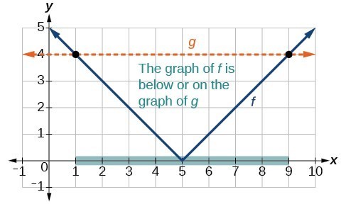
Figure 11. Graph to find the points satisfying an absolute value inequality.
We can see the following:
For absolute value inequalities,
The [latex]<\\[/latex] or [latex]>\\[/latex] symbol may be replaced by [latex]\le \text{ or }\ge \\[/latex].
So, for this example, we could use this alternative approach.
Solve [latex]|x+2|\le 6\\[/latex].
Given the function [latex]f\left(x\right)=-\frac{1}{2}|4x - 5|+3\\[/latex], determine the [latex]x\text{-}\\[/latex] values for which the function values are negative.
We are trying to determine where [latex]f\left(x\right)<0\\[/latex], which is when [latex]-\frac{1}{2}\text{ }|4x - 5|+3<0\\[/latex]. We begin by isolating the absolute value.
Next we solve for the equality [latex]|4x - 5|=6\\[/latex].
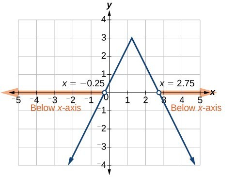
Figure 12
Now, we can examine the graph of [latex]f\\[/latex] to observe where the output is negative. We will observe where the branches are below the x-axis. Notice that it is not even important exactly what the graph looks like, as long as we know that it crosses the horizontal axis at [latex]x=-\frac{1}{4}\\[/latex] and [latex]x=\frac{11}{4}\\[/latex] and that the graph has been reflected vertically.
We observe that the graph of the function is below the x-axis left of [latex]x=-\frac{1}{4}\\[/latex] and right of [latex]x=\frac{11}{4}\\[/latex]. This means the function values are negative to the left of the first horizontal intercept at [latex]x=-\frac{1}{4}\\[/latex], and negative to the right of the second intercept at [latex]x=\frac{11}{4}\\[/latex]. This gives us the solution to the inequality.
In interval notation, this would be [latex]\left(-\infty ,-0.25\right)\cup \left(2.75,\infty \right)\\[/latex].
Solve [latex]-2|k - 4|\le -6\\[/latex].
1. How do you solve an absolute value equation?
2. How can you tell whether an absolute value function has two x-intercepts without graphing the function?
3. When solving an absolute value function, the isolated absolute value term is equal to a negative number. What does that tell you about the graph of the absolute value function?
4. How can you use the graph of an absolute value function to determine the x-values for which the function values are negative?
5. How do you solve an absolute value inequality algebraically?
6. Describe all numbers [latex]x\\[/latex] that are at a distance of 4 from the number 8. Express this using absolute value notation.
7. Describe all numbers [latex]x\\[/latex] that are at a distance of [latex]\frac{1}{2}\\[/latex] from the number −4. Express this using absolute value notation.
8. Describe the situation in which the distance that point [latex]x[/latex] is from 10 is at least 15 units. Express this using absolute value notation.
9. Find all function values [latex]f\left(x\right)\\[/latex] such that the distance from [latex]f\left(x\right)\\[/latex] to the value 8 is less than 0.03 units. Express this using absolute value notation.
For the following exercises, solve the equations below and express the answer using set notation.
10. [latex]|x+3|=9\\[/latex]
11. [latex]|6-x|=5\\[/latex]
12. [latex]|5x - 2|=11\\[/latex]
13. [latex]|4x - 2|=11\\[/latex]
14. [latex]2|4-x|=7\\[/latex]
15. [latex]3|5-x|=5\\[/latex]
16. [latex]3|x+1|-4=5\\[/latex]
17. [latex]5|x - 4|-7=2\\[/latex]
18. [latex]0=-|x - 3|+2\\[/latex]
19. [latex]2|x - 3|+1=2\\[/latex]
20. [latex]|3x - 2|=7\\[/latex]
21. [latex]|3x - 2|=-7\\[/latex]
22. [latex]\left|\frac{1}{2}x - 5\right|=11\\[/latex]
23. [latex]\left|\frac{1}{3}x+5\right|=14\\[/latex]
24. [latex]-\left|\frac{1}{3}x+5\right|+14=0\\[/latex]
For the following exercises, find the x- and y-intercepts of the graphs of each function.
25. [latex]f\left(x\right)=2|x+1|-10\\[/latex]
26. [latex]f\left(x\right)=4|x - 3|+4\\[/latex]
27. [latex]f\left(x\right)=-3|x - 2|-1\\[/latex]
28. [latex]f\left(x\right)=-2|x+1|+6\\[/latex]
For the following exercises, solve each inequality and write the solution in interval notation.
29. [latex]\left|x - 2\right|>10\\[/latex]
30. [latex]2|v - 7|-4\ge 42\\[/latex]
31. [latex]|3x - 4|\le 8\\[/latex]
32. [latex]|x - 4|\ge 8\\[/latex]
33. [latex]|3x - 5|\ge 13\\[/latex]
34. [latex]|3x - 5|\ge -13\\[/latex]
35. [latex]\left|\frac{3}{4}x - 5\right|\ge 7\\[/latex]
36. [latex]\left|\frac{3}{4}x - 5\right|+1\le 16\\[/latex]
For the following exercises, graph the absolute value function. Plot at least five points by hand for each graph.
37. [latex]y=|x - 1|\\[/latex]
38. [latex]y=|x+1|\\[/latex]
39. [latex]y=|x|+1\\[/latex]
For the following exercises, graph the given functions by hand.
40. [latex]y=|x|-2\\[/latex]
41. [latex]y=-|x|\\[/latex]
42. [latex]y=-|x|-2\\[/latex]
43. [latex]y=-|x - 3|-2\\[/latex]
44. [latex]f\left(x\right)=-|x - 1|-2\\[/latex]
45. [latex]f\left(x\right)=-|x+3|+4\\[/latex]
46. [latex]f\left(x\right)=2|x+3|+1\\[/latex]
47. [latex]f\left(x\right)=3|x - 2|+3\\[/latex]
48. [latex]f\left(x\right)=|2x - 4|-3\\[/latex]
49. [latex]f\left(x\right)=|3x+9|+2\\[/latex]
50. [latex]f\left(x\right)=-|x - 1|-3\\[/latex]
51. [latex]f\left(x\right)=-|x+4|-3\\[/latex]
52. [latex]f\left(x\right)=\frac{1}{2}\left|x+4\right|-3\\[/latex]
53. Use a graphing utility to graph [latex]f\left(x\right)=10|x - 2|\\[/latex] on the viewing window [latex]\left[0,4\right]\\[/latex]. Identify the corresponding range. Show the graph.
54. Use a graphing utility to graph [latex]f\left(x\right)=-100|x|+100\\[/latex] on the viewing window [latex]\left[-5,5\right]\\[/latex]. Identify the corresponding range. Show the graph.
For the following exercises, graph each function using a graphing utility. Specify the viewing window.
55. [latex]f\left(x\right)=\left(-0.1\right)\left|0.1\left(0.2-x\right)\right|+0.3\\[/latex]
56. [latex]f\left(x\right)=4\times {10}^{9}\left|x-\left(5\times {10}^{9}\right)\right|+2\times {10}^{9}\\[/latex]
For the following exercises, solve the inequality.
57. [latex]\left|-2x-\frac{2}{3}\left(x+1\right)\right|+3>-1\\[/latex]
58. If possible, find all values of [latex]a\\[/latex] such that there are no [latex]x\text{-}\\[/latex] intercepts for [latex]f\left(x\right)=2|x+1|+a\\[/latex].
59. If possible, find all values of [latex]a\\[/latex] such that there are no [latex]y\\[/latex] -intercepts for [latex]f\left(x\right)=2|x+1|+a\\[/latex].
60. Cities A and B are on the same east-west line. Assume that city A is located at the origin. If the distance from city A to city B is at least 100 miles and [latex]x\\[/latex] represents the distance from city B to city A, express this using absolute value notation.
61. The true proportion [latex]p\\[/latex] of people who give a favorable rating to Congress is 8% with a margin of error of 1.5%. Describe this statement using an absolute value equation.
62. Students who score within 18 points of the number 82 will pass a particular test. Write this statement using absolute value notation and use the variable [latex]x\\[/latex] for the score.
63. A machinist must produce a bearing that is within 0.01 inches of the correct diameter of 5.0 inches. Using [latex]x\\[/latex] as the diameter of the bearing, write this statement using absolute value notation.
64. The tolerance for a ball bearing is 0.01. If the true diameter of the bearing is to be 2.0 inches and the measured value of the diameter is [latex]x\\[/latex] inches, express the tolerance using absolute value notation.
1. [latex]|x - 2|\le 3\\[/latex]
2. using the variable [latex]p\\[/latex] for passing, [latex]|p - 80|\le 20\\[/latex]
3. [latex]f\left(x\right)=-|x+2|+3\\[/latex]
4. [latex]x=-1\\[/latex] or [latex]x=2\\[/latex]
5. [latex]f\left(0\right)=1\\[/latex], so the graph intersects the vertical axis at [latex]\left(0,1\right)\\[/latex]. [latex]f\left(x\right)=0\\[/latex] when [latex]x=-5\\[/latex] and [latex]x=1\\[/latex] so the graph intersects the horizontal axis at [latex]\left(-5,0\right)\\[/latex] and [latex]\left(1,0\right)\\[/latex].
6. [latex]4\le x\le 8\\[/latex]
7. [latex]k\le 1\\[/latex] or [latex]k\ge 7\\[/latex]; in interval notation, this would be [latex]\left(-\infty ,1\right]\cup \left[7,\infty \right)\\[/latex]
Solutions to Odd-Numbered Exercises
1. Isolate the absolute value term so that the equation is of the form [latex]|A|=B\\[/latex]. Form one equation by setting the expression inside the absolute value symbol, [latex]A\\[/latex], equal to the expression on the other side of the equation, [latex]B\\[/latex]. Form a second equation by setting [latex]A\\[/latex] equal to the opposite of the expression on the other side of the equation, -B. Solve each equation for the variable.
3. The graph of the absolute value function does not cross the [latex]x\\[/latex] -axis, so the graph is either completely above or completely below the [latex]x\\[/latex] -axis.
5. First determine the boundary points by finding the solution(s) of the equation. Use the boundary points to form possible solution intervals. Choose a test value in each interval to determine which values satisfy the inequality.
7. [latex]|x+4|=\frac{1}{2}\\[/latex]
9. [latex]|f\left(x\right)-8|<0.03\\[/latex]
11. [latex]\left\{1,11\right\}\\[/latex]
13. [latex]\left\{\frac{9}{4},\frac{13}{4}\right\}\\[/latex]
15. [latex]\left\{\frac{10}{3},\frac{20}{3}\right\}\\[/latex]
17. [latex]\left\{\frac{11}{5},\frac{29}{5}\right\}\\[/latex]
19. [latex]\left\{\frac{5}{2},\frac{7}{2}\right\}\\[/latex]
21. No solution
23. [latex]\left\{-57,27\right\}\\[/latex]
25. [latex]\left(0,-8\right);\left(-6,0\right),\left(4,0\right)\\[/latex]
27. [latex]\left(0,-7\right)\\[/latex]; no [latex]x\\[/latex] -intercepts
29. [latex]\left(-\infty ,-8\right)\cup \left(12,\infty \right)\\[/latex]
31. [latex]\frac{-4}{3}\le x\le 4\\[/latex]
33. [latex]\left(-\infty ,-\frac{8}{3}\right]\cup \left[6,\infty \right)\\[/latex]
35. [latex]\left(-\infty ,-\frac{8}{3}\right]\cup \left[16,\infty \right)\\[/latex]
37.
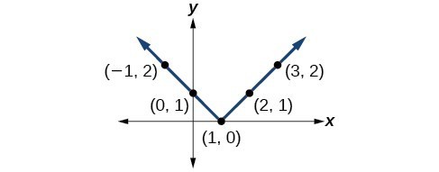
39.
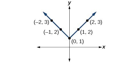
41.
43.
45.
47.
49.
51.
53. range: [latex]\left[0,20\right][/latex]
55. [latex]x\text{-}[/latex] intercepts:
57. [latex]\left(-\infty ,\infty \right)[/latex]
59. There is no solution for [latex]a[/latex] that will keep the function from having a [latex]y[/latex] -intercept. The absolute value function always crosses the [latex]y[/latex] -intercept when [latex]x=0[/latex].
61. [latex]|p - 0.08|\le 0.015[/latex]
63. [latex]|x - 5.0|\le 0.01[/latex]
By the end of this lesson, you will be able to:
A reversible heat pump is a climate-control system that is an air conditioner and a heater in a single device. Operated in one direction, it pumps heat out of a house to provide cooling. Operating in reverse, it pumps heat into the building from the outside, even in cool weather, to provide heating. As a heater, a heat pump is several times more efficient than conventional electrical resistance heating.
If some physical machines can run in two directions, we might ask whether some of the function “machines” we have been studying can also run backwards. Figure 1 provides a visual representation of this question. In this section, we will consider the reverse nature of functions.

Figure 1. Can a function “machine” operate in reverse?
Suppose a fashion designer traveling to Milan for a fashion show wants to know what the temperature will be. He is not familiar with the Celsius scale. To get an idea of how temperature measurements are related, he asks his assistant, Betty, to convert 75 degrees Fahrenheit to degrees Celsius. She finds the formula
and substitutes 75 for [latex]F[/latex] to calculate
Figure 2
Knowing that a comfortable 75 degrees Fahrenheit is about 24 degrees Celsius, he sends his assistant the week’s weather forecast for Milan, and asks her to convert all of the temperatures to degrees Fahrenheit.
At first, Betty considers using the formula she has already found to complete the conversions. After all, she knows her algebra, and can easily solve the equation for [latex]F[/latex] after substituting a value for [latex]C[/latex]. For example, to convert 26 degrees Celsius, she could write
After considering this option for a moment, however, she realizes that solving the equation for each of the temperatures will be awfully tedious. She realizes that since evaluation is easier than solving, it would be much more convenient to have a different formula, one that takes the Celsius temperature and outputs the Fahrenheit temperature.
The formula for which Betty is searching corresponds to the idea of an inverse function, which is a function for which the input of the original function becomes the output of the inverse function and the output of the original function becomes the input of the inverse function.
Given a function [latex]f\left(x\right)[/latex], we represent its inverse as [latex]{f}^{-1}\left(x\right)[/latex], read as [latex]``f[/latex] inverse of [latex]x.\text{``}[/latex] The raised [latex]-1[/latex] is part of the notation. It is not an exponent; it does not imply a power of [latex]-1[/latex] . In other words, [latex]{f}^{-1}\left(x\right)[/latex] does not mean [latex]\frac{1}{f\left(x\right)}[/latex] because [latex]\frac{1}{f\left(x\right)}[/latex] is the reciprocal of [latex]f[/latex] and not the inverse.
The “exponent-like” notation comes from an analogy between function composition and multiplication: just as [latex]{a}^{-1}a=1[/latex] (1 is the identity element for multiplication) for any nonzero number [latex]a[/latex], so [latex]{f}^{-1}\circ f\\[/latex] equals the identity function, that is,
This holds for all [latex]x[/latex] in the domain of [latex]f[/latex]. Informally, this means that inverse functions “undo” each other. However, just as zero does not have a reciprocal, some functions do not have inverses.
Given a function [latex]f\left(x\right)[/latex], we can verify whether some other function [latex]g\left(x\right)[/latex] is the inverse of [latex]f\left(x\right)[/latex] by checking whether either [latex]g\left(f\left(x\right)\right)=x[/latex] or [latex]f\left(g\left(x\right)\right)=x[/latex] is true. We can test whichever equation is more convenient to work with because they are logically equivalent (that is, if one is true, then so is the other.)
For example, [latex]y=4x[/latex] and [latex]y=\frac{1}{4}x\\[/latex] are inverse functions.
and
A few coordinate pairs from the graph of the function [latex]y=4x[/latex] are (−2, −8), (0, 0), and (2, 8). A few coordinate pairs from the graph of the function [latex]y=\frac{1}{4}x\\[/latex] are (−8, −2), (0, 0), and (8, 2). If we interchange the input and output of each coordinate pair of a function, the interchanged coordinate pairs would appear on the graph of the inverse function.
For any one-to-one function [latex]f\left(x\right)=y[/latex], a function [latex]{f}^{-1}\left(x\right)[/latex] is an inverse function of [latex]f[/latex] if [latex]{f}^{-1}\left(y\right)=x[/latex]. This can also be written as [latex]{f}^{-1}\left(f\left(x\right)\right)=x[/latex] for all [latex]x[/latex] in the domain of [latex]f[/latex]. It also follows that [latex]f\left({f}^{-1}\left(x\right)\right)=x[/latex] for all [latex]x[/latex] in the domain of [latex]{f}^{-1}[/latex] if [latex]{f}^{-1}[/latex] is the inverse of [latex]f[/latex].
The notation [latex]{f}^{-1}[/latex] is read [latex]\text{``}f[/latex] inverse.” Like any other function, we can use any variable name as the input for [latex]{f}^{-1}[/latex], so we will often write [latex]{f}^{-1}\left(x\right)[/latex], which we read as [latex]``f[/latex] inverse of [latex]x.''[/latex]
Keep in mind that
and not all functions have inverses.
If for a particular one-to-one function [latex]f\left(2\right)=4[/latex] and [latex]f\left(5\right)=12[/latex], what are the corresponding input and output values for the inverse function?
The inverse function reverses the input and output quantities, so if
Alternatively, if we want to name the inverse function [latex]g[/latex], then [latex]g\left(4\right)=2[/latex] and [latex]g\left(12\right)=5[/latex].
Notice that if we show the coordinate pairs in a table form, the input and output are clearly reversed.
| [latex]\left(x,f\left(x\right)\right)[/latex] | [latex]\left(x,g\left(x\right)\right)[/latex] |
|---|---|
| [latex]\left(2,4\right)[/latex] | [latex]\left(4,2\right)[/latex] |
| [latex]\left(5,12\right)[/latex] | [latex]\left(12,5\right)[/latex] |
Given that [latex]{h}^{-1}\left(6\right)=2[/latex], what are the corresponding input and output values of the original function [latex]h?[/latex]
If [latex]f\left(x\right)=\frac{1}{x+2}[/latex] and [latex]g\left(x\right)=\frac{1}{x}-2[/latex], is [latex]g={f}^{-1}?[/latex]
[latex]\begin{cases} g\left(f\left(x\right)\right)=\frac{1}{\left(\frac{1}{x+2}\right)}{-2 }\hfill\\={ x }+{ 2 } -{ 2 }\hfill\\={ x }\hfill \end{cases}\\[/latex]
so
This is enough to answer yes to the question, but we can also verify the other formula.
Notice the inverse operations are in reverse order of the operations from the original function.
If [latex]f\left(x\right)={x}^{3}-4[/latex] and [latex]g\left(x\right)=\sqrt[3]{x+4}[/latex], is [latex]g={f}^{-1}?[/latex]
If [latex]f\left(x\right)={x}^{3}[/latex] (the cube function) and [latex]g\left(x\right)=\frac{1}{3}x[/latex], is [latex]g={f}^{-1}?\\[/latex]
[latex]f\left(g\left(x\right)\right)=\frac{{x}^{3}}{27}\ne x\\[/latex]
No, the functions are not inverses.
The correct inverse to the cube is, of course, the cube root [latex]\sqrt[3]{x}={x}^{\frac{1}{3}}\\[/latex], that is, the one-third is an exponent, not a multiplier.
If [latex]f\left(x\right)={\left(x - 1\right)}^{3}\text{and}g\left(x\right)=\sqrt[3]{x}+1\\[/latex], is [latex]g={f}^{-1}?\\[/latex]
The outputs of the function [latex]f[/latex] are the inputs to [latex]{f}^{-1}[/latex], so the range of [latex]f[/latex] is also the domain of [latex]{f}^{-1}[/latex]. Likewise, because the inputs to [latex]f[/latex] are the outputs of [latex]{f}^{-1}[/latex], the domain of [latex]f[/latex] is the range of [latex]{f}^{-1}[/latex]. We can visualize the situation.
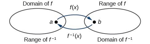
Figure 3. Domain and range of a function and its inverse
When a function has no inverse function, it is possible to create a new function where that new function on a limited domain does have an inverse function. For example, the inverse of [latex]f\left(x\right)=\sqrt{x}[/latex] is [latex]{f}^{-1}\left(x\right)={x}^{2}[/latex], because a square “undoes” a square root; but the square is only the inverse of the square root on the domain [latex]\left[0,\infty \right)[/latex], since that is the range of [latex]f\left(x\right)=\sqrt{x}[/latex].
We can look at this problem from the other side, starting with the square (toolkit quadratic) function [latex]f\left(x\right)={x}^{2}[/latex]. If we want to construct an inverse to this function, we run into a problem, because for every given output of the quadratic function, there are two corresponding inputs (except when the input is 0). For example, the output 9 from the quadratic function corresponds to the inputs 3 and –3. But an output from a function is an input to its inverse; if this inverse input corresponds to more than one inverse output (input of the original function), then the “inverse” is not a function at all! To put it differently, the quadratic function is not a one-to-one function; it fails the horizontal line test, so it does not have an inverse function. In order for a function to have an inverse, it must be a one-to-one function.
In many cases, if a function is not one-to-one, we can still restrict the function to a part of its domain on which it is one-to-one. For example, we can make a restricted version of the square function [latex]f\left(x\right)={x}^{2}[/latex] with its range limited to [latex]\left[0,\infty \right)[/latex], which is a one-to-one function (it passes the horizontal line test) and which has an inverse (the square-root function).
If [latex]f\left(x\right)={\left(x - 1\right)}^{2}[/latex] on [latex]\left[1,\infty \right)[/latex], then the inverse function is [latex]{f}^{-1}\left(x\right)=\sqrt{x}+1[/latex].
Q & A
Is it possible for a function to have more than one inverse?
No. If two supposedly different functions, say, [latex]g[/latex] and [latex]h[/latex], both meet the definition of being inverses of another function [latex]f[/latex], then you can prove that [latex]g=h[/latex]. We have just seen that some functions only have inverses if we restrict the domain of the original function. In these cases, there may be more than one way to restrict the domain, leading to different inverses. However, on any one domain, the original function still has only one unique inverse.
The range of a function [latex]f\left(x\right)[/latex] is the domain of the inverse function [latex]{f}^{-1}\left(x\right)[/latex].
The domain of [latex]f\left(x\right)[/latex] is the range of [latex]{f}^{-1}\left(x\right)[/latex].
Identify which of the toolkit functions besides the quadratic function are not one-to-one, and find a restricted domain on which each function is one-to-one, if any. The toolkit functions are reviewed below. We restrict the domain in such a fashion that the function assumes all y-values exactly once.
| Constant | Identity | Quadratic | Cubic | Reciprocal |
| [latex]f\left(x\right)=c[/latex] | [latex]f\left(x\right)=x[/latex] | [latex]f\left(x\right)={x}^{2}[/latex] | [latex]f\left(x\right)={x}^{3}[/latex] | [latex]f\left(x\right)=\frac{1}{x}[/latex] |
| Reciprocal squared | Cube root | Square root | Absolute value | |
| [latex]f\left(x\right)=\frac{1}{{x}^{2}}[/latex] | [latex]f\left(x\right)=\sqrt[3]{x}[/latex] | [latex]f\left(x\right)=\sqrt{x}[/latex] | [latex]f\left(x\right)=|x|[/latex] |
The constant function is not one-to-one, and there is no domain (except a single point) on which it could be one-to-one, so the constant function has no meaningful inverse.
The absolute value function can be restricted to the domain [latex]\left[0,\infty \right)[/latex], where it is equal to the identity function.
The reciprocal-squared function can be restricted to the domain [latex]\left(0,\infty \right)[/latex].
We can see that these functions (if unrestricted) are not one-to-one by looking at their graphs. They both would fail the horizontal line test. However, if a function is restricted to a certain domain so that it passes the horizontal line test, then in that restricted domain, it can have an inverse.
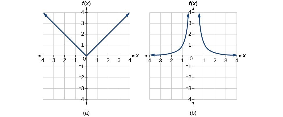
Figure 4. (a) Absolute value (b) Reciprocal squared
The domain of function [latex]f[/latex] is [latex]\left(1,\infty \right)[/latex] and the range of function [latex]f[/latex] is [latex]\left(\mathrm{-\infty },-2\right)[/latex]. Find the domain and range of the inverse function.
Once we have a one-to-one function, we can evaluate its inverse at specific inverse function inputs or construct a complete representation of the inverse function in many cases.
Suppose we want to find the inverse of a function represented in table form. Remember that the domain of a function is the range of the inverse and the range of the function is the domain of the inverse. So we need to interchange the domain and range.
Each row (or column) of inputs becomes the row (or column) of outputs for the inverse function. Similarly, each row (or column) of outputs becomes the row (or column) of inputs for the inverse function.
A function [latex]f\left(t\right)[/latex] is given below, showing distance in miles that a car has traveled in [latex]t[/latex] minutes. Find and interpret [latex]{f}^{-1}\left(70\right)[/latex].
| [latex]t\text{ (minutes)}[/latex] | 30 | 50 | 70 | 90 |
| [latex]f\left(t\right)\text{ (miles)}[/latex] | 20 | 40 | 60 | 70 |
The inverse function takes an output of [latex]f[/latex] and returns an input for [latex]f[/latex]. So in the expression [latex]{f}^{-1}\left(70\right)[/latex], 70 is an output value of the original function, representing 70 miles. The inverse will return the corresponding input of the original function [latex]f[/latex], 90 minutes, so [latex]{f}^{-1}\left(70\right)=90[/latex]. The interpretation of this is that, to drive 70 miles, it took 90 minutes.
Alternatively, recall that the definition of the inverse was that if [latex]f\left(a\right)=b[/latex], then [latex]{f}^{-1}\left(b\right)=a[/latex]. By this definition, if we are given [latex]{f}^{-1}\left(70\right)=a[/latex], then we are looking for a value [latex]a[/latex] so that [latex]f\left(a\right)=70[/latex]. In this case, we are looking for a [latex]t[/latex] so that [latex]f\left(t\right)=70[/latex], which is when [latex]t=90[/latex].
Using the table below, find and interpret (a) [latex]\text{ }f\left(60\right)[/latex], and (b) [latex]\text{ }{f}^{-1}\left(60\right)[/latex].
| [latex]t\text{ (minutes)}[/latex] | 30 | 50 | 60 | 70 | 90 |
| [latex]f\left(t\right)\text{ (miles)}[/latex] | 20 | 40 | 50 | 60 | 70 |
We saw in Functions and Function Notation that the domain of a function can be read by observing the horizontal extent of its graph. We find the domain of the inverse function by observing the vertical extent of the graph of the original function, because this corresponds to the horizontal extent of the inverse function. Similarly, we find the range of the inverse function by observing the horizontal extent of the graph of the original function, as this is the vertical extent of the inverse function. If we want to evaluate an inverse function, we find its input within its domain, which is all or part of the vertical axis of the original function’s graph.
A function [latex]g\left(x\right)[/latex] is given in Figure 5. Find [latex]g\left(3\right)[/latex] and [latex]{g}^{-1}\left(3\right)[/latex].
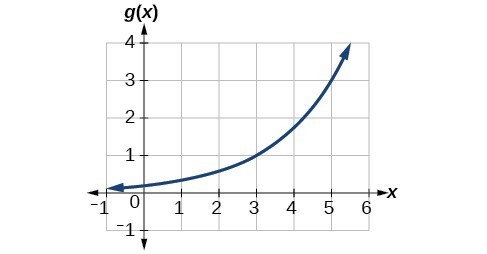
Figure 5
To evaluate [latex]g\left(3\right)[/latex], we find 3 on the x-axis and find the corresponding output value on the y-axis. The point [latex]\left(3,1\right)[/latex] tells us that [latex]g\left(3\right)=1[/latex].
To evaluate [latex]{g}^{-1}\left(3\right)[/latex], recall that by definition [latex]{g}^{-1}\left(3\right)[/latex] means the value of x for which [latex]g\left(x\right)=3[/latex]. By looking for the output value 3 on the vertical axis, we find the point [latex]\left(5,3\right)[/latex] on the graph, which means [latex]g\left(5\right)=3[/latex], so by definition, [latex]{g}^{-1}\left(3\right)=5[/latex].
Figure 6
Using the graph in Example 6, (a) find [latex]{g}^{-1}\left(1\right)[/latex], and (b) estimate [latex]{g}^{-1}\left(4\right)[/latex].
Sometimes we will need to know an inverse function for all elements of its domain, not just a few. If the original function is given as a formula— for example, [latex]y[/latex] as a function of [latex]x\text{-\hspace{0.17em}}[/latex] we can often find the inverse function by solving to obtain [latex]x[/latex] as a function of [latex]y[/latex].
Find a formula for the inverse function that gives Fahrenheit temperature as a function of Celsius temperature.
[latex]\begin{cases}\hfill{ C }=\frac{5}{9}\left(F - 32\right)\hfill \\ C\cdot \frac{9}{5}=F - 32\hfill \\ F=\frac{9}{5}C+32\hfill \end{cases}[/latex]
By solving in general, we have uncovered the inverse function. If
then
In this case, we introduced a function [latex]h[/latex] to represent the conversion because the input and output variables are descriptive, and writing [latex]{C}^{-1}[/latex] could get confusing.
Solve for [latex]x[/latex] in terms of [latex]y[/latex] given [latex]y=\frac{1}{3}\left(x - 5\right)\\[/latex]
Find the inverse of the function [latex]f\left(x\right)=\frac{2}{x - 3}+4\\[/latex].
So [latex]{f}^{-1}\left(y\right)=\frac{2}{y - 4}+3\\[/latex] or [latex]{f}^{-1}\left(x\right)=\frac{2}{x - 4}+3\\[/latex].
The domain and range of [latex]f[/latex] exclude the values 3 and 4, respectively. [latex]f[/latex] and [latex]{f}^{-1}[/latex] are equal at two points but are not the same function, as we can see by creating the table below.
| [latex]x[/latex] | 1 | 2 | 5 | [latex]{f}^{-1}\left(y\right)[/latex] |
| [latex]f\left(x\right)[/latex] | 3 | 2 | 5 | [latex]y[/latex] |
Find the inverse of the function [latex]f\left(x\right)=2+\sqrt{x - 4}[/latex].
So [latex]{f}^{-1}\left(x\right)={\left(x - 2\right)}^{2}+4[/latex].
The domain of [latex]f[/latex] is [latex]\left[4,\infty \right)[/latex]. Notice that the range of [latex]f[/latex] is [latex]\left[2,\infty \right)[/latex], so this means that the domain of the inverse function [latex]{f}^{-1}[/latex] is also [latex]\left[2,\infty \right)[/latex].
The formula we found for [latex]{f}^{-1}\left(x\right)[/latex] looks like it would be valid for all real [latex]x[/latex]. However, [latex]{f}^{-1}[/latex] itself must have an inverse (namely, [latex]f[/latex] ) so we have to restrict the domain of [latex]{f}^{-1}[/latex] to [latex]\left[2,\infty \right)[/latex] in order to make [latex]{f}^{-1}[/latex] a one-to-one function. This domain of [latex]{f}^{-1}[/latex] is exactly the range of [latex]f[/latex].
What is the inverse of the function [latex]f\left(x\right)=2-\sqrt{x}?[/latex] State the domains of both the function and the inverse function.
Now that we can find the inverse of a function, we will explore the graphs of functions and their inverses. Let us return to the quadratic function [latex]f\left(x\right)={x}^{2}[/latex] restricted to the domain [latex]\left[0,\infty \right)[/latex], on which this function is one-to-one, and graph it as in Figure 7.
Figure 7. Quadratic function with domain restricted to [0, ∞).
Restricting the domain to [latex]\left[0,\infty \right)[/latex] makes the function one-to-one (it will obviously pass the horizontal line test), so it has an inverse on this restricted domain.
We already know that the inverse of the toolkit quadratic function is the square root function, that is, [latex]{f}^{-1}\left(x\right)=\sqrt{x}[/latex]. What happens if we graph both [latex]f\text{ }[/latex] and [latex]{f}^{-1}[/latex] on the same set of axes, using the [latex]x\text{-}[/latex] axis for the input to both [latex]f\text{ and }{f}^{-1}?[/latex]
We notice a distinct relationship: The graph of [latex]{f}^{-1}\left(x\right)[/latex] is the graph of [latex]f\left(x\right)[/latex] reflected about the diagonal line [latex]y=x[/latex], which we will call the identity line, shown in Figure 8.
Figure 8. Square and square-root functions on the non-negative domain
This relationship will be observed for all one-to-one functions, because it is a result of the function and its inverse swapping inputs and outputs. This is equivalent to interchanging the roles of the vertical and horizontal axes.
Given the graph of [latex]f\left(x\right)[/latex], sketch a graph of [latex]{f}^{-1}\left(x\right)[/latex].
Figure 9
This is a one-to-one function, so we will be able to sketch an inverse. Note that the graph shown has an apparent domain of [latex]\left(0,\infty \right)[/latex] and range of [latex]\left(-\infty ,\infty \right)[/latex], so the inverse will have a domain of [latex]\left(-\infty ,\infty \right)[/latex] and range of [latex]\left(0,\infty \right)[/latex].
If we reflect this graph over the line [latex]y=x[/latex], the point [latex]\left(1,0\right)[/latex] reflects to [latex]\left(0,1\right)[/latex] and the point [latex]\left(4,2\right)[/latex] reflects to [latex]\left(2,4\right)[/latex]. Sketching the inverse on the same axes as the original graph gives us the result in Figure 10.
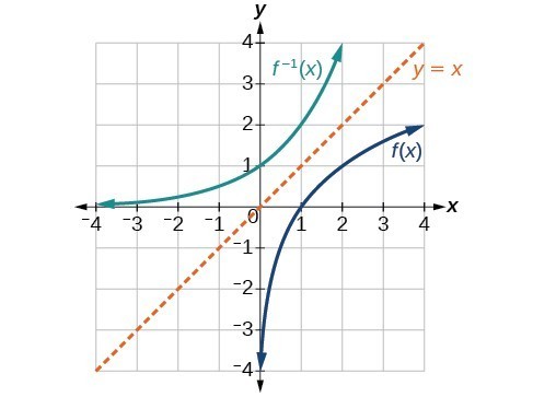
Figure 10. The function and its inverse, showing reflection about the identity line
Draw graphs of the functions [latex]f\text{ }[/latex] and [latex]\text{ }{f}^{-1}[/latex].
Q & A
Is there any function that is equal to its own inverse?
Yes. If [latex]f={f}^{-1}[/latex], then [latex]f\left(f\left(x\right)\right)=x[/latex], and we can think of several functions that have this property. The identity function does, and so does the reciprocal function, because
Any function [latex]f\left(x\right)=c-x[/latex], where [latex]c[/latex] is a constant, is also equal to its own inverse.
1. Describe why the horizontal line test is an effective way to determine whether a function is one-to-one?
2. Why do we restrict the domain of the function [latex]f\left(x\right)={x}^{2}[/latex] to find the function’s inverse?
3. Can a function be its own inverse? Explain.
4. Are one-to-one functions either always increasing or always decreasing? Why or why not?
5. How do you find the inverse of a function algebraically?
6. Show that the function [latex]f\left(x\right)=a-x[/latex] is its own inverse for all real numbers [latex]a[/latex].
For the following exercises, find [latex]{f}^{-1}\left(x\right)[/latex] for each function.
7. [latex]f\left(x\right)=x+3[/latex]
8. [latex]f\left(x\right)=x+5[/latex]
9. [latex]f\left(x\right)=2-x[/latex]
10. [latex]f\left(x\right)=3-x[/latex]
11. [latex]f\left(x\right)=\frac{x}{x+2}\\[/latex]
12. [latex]f\left(x\right)=\frac{2x+3}{5x+4}[/latex]
For the following exercises, find a domain on which each function [latex]f[/latex] is one-to-one and non-decreasing. Write the domain in interval notation. Then find the inverse of [latex]f[/latex] restricted to that domain.
13. [latex]f\left(x\right)={\left(x+7\right)}^{2}[/latex]
14. [latex]f\left(x\right)={\left(x - 6\right)}^{2}[/latex]
15. [latex]f\left(x\right)={x}^{2}-5[/latex]
16. Given [latex]f\left(x\right)=\frac{x}{2}+x\\[/latex] and [latex]g\left(x\right)=\frac{2x}{1-x}\\[/latex]
a. Find [latex]f\left(g\left(x\right)\right)[/latex] and [latex]g\left(f\left(x\right)\right)\\[/latex]
b. What does the answer tell us about the relationship between [latex]f\left(x\right)[/latex] and [latex]g\left(x\right)?[/latex]
For the following exercises, use function composition to verify that [latex]f\left(x\right)[/latex] and [latex]g\left(x\right)[/latex] are inverse functions.
17. [latex]f\left(x\right)=\sqrt[3]{x - 1}[/latex] and [latex]g\left(x\right)={x}^{3}+1[/latex]
18. [latex]f\left(x\right)=-3x+5[/latex] and [latex]g\left(x\right)=\frac{x - 5}{-3}[/latex]
For the following exercises, use a graphing utility to determine whether each function is one-to-one.
19. [latex]f\left(x\right)=\sqrt{x}[/latex]
20. [latex]f\left(x\right)=\sqrt[3]{3x+1}[/latex]
21. [latex]f\left(x\right)=-5x+1[/latex]
22. [latex]f\left(x\right)={x}^{3}-27[/latex]
For the following exercises, determine whether the graph represents a one-to-one function.
23.
24.
For the following exercises, use the graph of [latex]f[/latex] shown in [link].
25. Find [latex]f\left(0\right)[/latex].
26. Solve [latex]f\left(x\right)=0[/latex].
27. Find [latex]{f}^{-1}\left(0\right)[/latex].
28. Solve [latex]{f}^{-1}\left(x\right)=0[/latex].
For the following exercises, use the graph of the one-to-one function shown below.
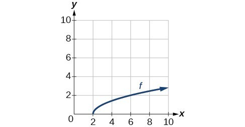
29. Sketch the graph of [latex]{f}^{-1}[/latex].
30. Find [latex]f\left(6\right)\text{ and }{f}^{-1}\left(2\right)[/latex].
31. If the complete graph of [latex]f[/latex] is shown, find the domain of [latex]f[/latex].
32. If the complete graph of [latex]f[/latex] is shown, find the range of [latex]f[/latex].
For the following exercises, evaluate or solve, assuming that the function [latex]f[/latex] is one-to-one.
33. If [latex]f\left(6\right)=7[/latex], find [latex]{f}^{-1}\left(7\right)[/latex].
34. If [latex]f\left(3\right)=2[/latex], find [latex]{f}^{-1}\left(2\right)[/latex].
35. If [latex]{f}^{-1}\left(-4\right)=-8[/latex], find [latex]f\left(-8\right)[/latex].
36. If [latex]{f}^{-1}\left(-2\right)=-1[/latex], find [latex]f\left(-1\right)[/latex].
For the following exercises, use the values listed in the table below to evaluate or solve.
| [latex]x[/latex] | [latex]f\left(x\right)[/latex] |
| 0 | 8 |
| 1 | 0 |
| 2 | 7 |
| 3 | 4 |
| 4 | 2 |
| 5 | 6 |
| 6 | 5 |
| 7 | 3 |
| 8 | 9 |
| 9 | 1 |
37. Find [latex]f\left(1\right)[/latex].
38. Solve [latex]f\left(x\right)=3[/latex].
39. Find [latex]{f}^{-1}\left(0\right)[/latex].
40. Solve [latex]{f}^{-1}\left(x\right)=7[/latex].
41. Use the tabular representation of [latex]f[/latex] to create a table for [latex]{f}^{-1}\left(x\right)[/latex].
| [latex]x[/latex] | 3 | 6 | 9 | 13 | 14 |
| [latex]f\left(x\right)[/latex] | 1 | 4 | 7 | 12 | 16 |
For the following exercises, find the inverse function. Then, graph the function and its inverse.
42. [latex]f\left(x\right)=\frac{3}{x - 2}[/latex]
43. [latex]f\left(x\right)={x}^{3}-1[/latex]
44. Find the inverse function of [latex]f\left(x\right)=\frac{1}{x - 1}[/latex]. Use a graphing utility to find its domain and range. Write the domain and range in interval notation.
45. To convert from [latex]x[/latex] degrees Celsius to [latex]y[/latex] degrees Fahrenheit, we use the formula [latex]f\left(x\right)=\frac{9}{5}x+32[/latex]. Find the inverse function, if it exists, and explain its meaning.
46. The circumference [latex]C[/latex] of a circle is a function of its radius given by [latex]C\left(r\right)=2\pi r[/latex]. Express the radius of a circle as a function of its circumference. Call this function [latex]r\left(C\right)[/latex]. Find [latex]r\left(36\pi \right)[/latex] and interpret its meaning.
47. A car travels at a constant speed of 50 miles per hour. The distance the car travels in miles is a function of time, [latex]t[/latex], in hours given by [latex]d\left(t\right)=50t[/latex]. Find the inverse function by expressing the time of travel in terms of the distance traveled. Call this function [latex]t\left(d\right)[/latex]. Find [latex]t\left(180\right)[/latex] and interpret its meaning.
1. [latex]h\left(2\right)=6[/latex]
2. Yes
3. Yes
4. The domain of function [latex]{f}^{-1}[/latex] is [latex]\left(-\infty \text{,}-2\right)[/latex] and the range of function [latex]{f}^{-1}[/latex] is [latex]\left(1,\infty \right)[/latex].
5. a. [latex]f\left(60\right)=50[/latex]. In 60 minutes, 50 miles are traveled.
b. [latex]{f}^{-1}\left(60\right)=70[/latex]. To travel 60 miles, it will take 70 minutes.
6. a. 3; b. 5.6
7. [latex]x=3y+5[/latex]
8. [latex]{f}^{-1}\left(x\right)={\left(2-x\right)}^{2};\text{domain}\text{of}f:\left[0,\infty \right);\text{domain}\text{of}{f}^{-1}:\left(-\infty ,2\right]\\[/latex]
9.

1. Each output of a function must have exactly one output for the function to be one-to-one. If any horizontal line crosses the graph of a function more than once, that means that [latex]y[/latex] -values repeat and the function is not one-to-one. If no horizontal line crosses the graph of the function more than once, then no [latex]y[/latex] -values repeat and the function is one-to-one.
3. Yes. For example, [latex]f\left(x\right)=\frac{1}{x}\\[/latex] is its own inverse.
5. Given a function [latex]y=f\left(x\right)[/latex], solve for [latex]x[/latex] in terms of [latex]y[/latex]. Interchange the [latex]x[/latex] and [latex]y[/latex]. Solve the new equation for [latex]y[/latex]. The expression for [latex]y[/latex] is the inverse, [latex]y={f}^{-1}\left(x\right)[/latex].
7. [latex]{f}^{-1}\left(x\right)=x - 3[/latex]
9. [latex]{f}^{-1}\left(x\right)=2-x[/latex]
11. [latex]{f}^{-1}\left(x\right)=\frac{-2x}{x - 1}\\[/latex]
13. domain of [latex]f\left(x\right):\left[-7,\infty \right);{f}^{-1}\left(x\right)=\sqrt{x}-7[/latex]
15. domain of [latex]f\left(x\right):\left[0,\infty \right);{f}^{-1}\left(x\right)=\sqrt{x+5}\\[/latex]
17. [latex] f\left(g\left(x\right)\right)=x,g\left(f\left(x\right)\right)=x[/latex]
19. one-to-one
21. one-to-one
23. not one-to-one
25. [latex]3[/latex]
27. [latex]2[/latex]
29.

31. [latex]\left[2,10\right][/latex]
33. [latex]6[/latex]
35. [latex]-4[/latex]
37. [latex]0[/latex]
39. [latex]1[/latex]
41.
| [latex]x[/latex] | 1 | 4 | 7 | 12 | 16 |
| [latex]{f}^{-1}\left(x\right)\\[/latex] | 3 | 6 | 9 | 13 | 14 |
43. [latex]{f}^{-1}\left(x\right)={\left(1+x\right)}^{1/3}\\[/latex]

45. [latex]{f}^{-1}\left(x\right)=\frac{5}{9}\left(x - 32\right)\\[/latex]. Given the Fahrenheit temperature, [latex]x[/latex], this formula allows you to calculate the Celsius temperature.
47. [latex]t\left(d\right)=\frac{d}{50}\\[/latex], [latex]t\left(180\right)=\frac{180}{50}\\[/latex]. The time for the car to travel 180 miles is 3.6 hours.
By the end of this lesson, you will be able to:
A bamboo forest in China (credit: “JFXie”/Flickr)
Imagine placing a plant in the ground one day and finding that it has doubled its height just a few days later. Although it may seem incredible, this can happen with certain types of bamboo species. These members of the grass family are the fastest-growing plants in the world. One species of bamboo has been observed to grow nearly 1.5 inches every hour.1 In a twenty-four hour period, this bamboo plant grows about 36 inches, or an incredible 3 feet! A constant rate of change, such as the growth cycle of this bamboo plant, is a linear function.
Recall from Functions and Function Notation that a function is a relation that assigns to every element in the domain exactly one element in the range. Linear functions are a specific type of function that can be used to model many real-world applications, such as plant growth over time. In this chapter, we will explore linear functions, their graphs, and how to relate them to data.

Shanghai MagLev Train (credit: “kanegen”/Flickr)
Just as with the growth of a bamboo plant, there are many situations that involve constant change over time. Consider, for example, the first commercial maglev train in the world, the Shanghai MagLev Train. It carries passengers comfortably for a 30-kilometer trip from the airport to the subway station in only eight minutes. (http://www.chinahighlights.com/shanghai/transportation/maglev-train.htm)
Suppose a maglev train were to travel a long distance, and that the train maintains a constant speed of 83 meters per second for a period of time once it is 250 meters from the station. How can we analyze the train’s distance from the station as a function of time? In this section, we will investigate a kind of function that is useful for this purpose, and use it to investigate real-world situations such as the train’s distance from the station at a given point in time.
The function describing the train’s motion is a linear function, which is defined as a function with a constant rate of change, that is, a polynomial of degree 1. There are several ways to represent a linear function, including word form, function notation, tabular form, and graphical form. We will describe the train’s motion as a function using each method.
Let’s begin by describing the linear function in words. For the train problem we just considered, the following word sentence may be used to describe the function relationship.
The speed is the rate of change. Recall that a rate of change is a measure of how quickly the dependent variable changes with respect to the independent variable. The rate of change for this example is constant, which means that it is the same for each input value. As the time (input) increases by 1 second, the corresponding distance (output) increases by 83 meters. The train began moving at this constant speed at a distance of 250 meters from the station.
Another approach to representing linear functions is by using function notation. One example of function notation is an equation written in the form known as the slope-intercept form of a line, where [latex]x[/latex] is the input value, [latex]m[/latex] is the rate of change, and [latex]b[/latex] is the initial value of the dependent variable.
In the example of the train, we might use the notation [latex]D\left(t\right)[/latex] in which the total distance [latex]D[/latex]
is a function of the time [latex]t[/latex]. The rate, [latex]m[/latex], is 83 meters per second. The initial value of the dependent variable [latex]b[/latex] is the original distance from the station, 250 meters. We can write a generalized equation to represent the motion of the train.
A third method of representing a linear function is through the use of a table. The relationship between the distance from the station and the time is represented in the table in Figure 1. From the table, we can see that the distance changes by 83 meters for every 1 second increase in time.
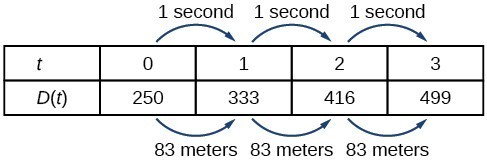
Figure 1. Tabular representation of the function D showing selected input and output values
Can the input in the previous example be any real number?
No. The input represents time, so while nonnegative rational and irrational numbers are possible, negative real numbers are not possible for this example. The input consists of non-negative real numbers.
Another way to represent linear functions is visually, using a graph. We can use the function relationship from above, [latex]D\left(t\right)=83t+250[/latex], to draw a graph, represented in the graph in Figure 2. Notice the graph is a line. When we plot a linear function, the graph is always a line.
The rate of change, which is constant, determines the slant, or slope of the line. The point at which the input value is zero is the vertical intercept, or y-intercept, of the line. We can see from the graph that the y-intercept in the train example we just saw is [latex]\left(0,250\right)[/latex] and represents the distance of the train from the station when it began moving at a constant speed.
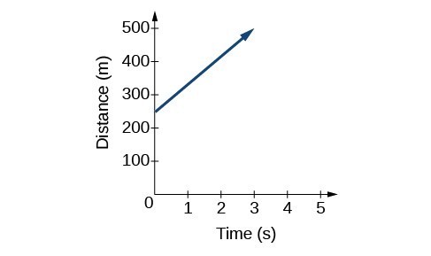
Figure 2. The graph of [latex]D\left(t\right)=83t+250[/latex]. Graphs of linear functions are lines because the rate of change is constant.
Notice that the graph of the train example is restricted, but this is not always the case. Consider the graph of the line [latex]f\left(x\right)=2{x}_{}+1[/latex]. Ask yourself what numbers can be input to the function, that is, what is the domain of the function? The domain is comprised of all real numbers because any number may be doubled, and then have one added to the product.
A linear function is a function whose graph is a line. Linear functions can be written in the slope-intercept form of a line
where [latex]b[/latex] is the initial or starting value of the function (when input, [latex]x=0[/latex]), and [latex]m[/latex] is the constant rate of change, or slope of the function. The y-intercept is at [latex]\left(0,b\right)[/latex].
The pressure, [latex]P[/latex], in pounds per square inch (PSI) on the diver in Figure 3 depends upon her depth below the water surface, [latex]d[/latex], in feet. This relationship may be modeled by the equation, [latex]P\left(d\right)=0.434d+14.696[/latex]. Restate this function in words.

Figure 3. (credit: Ilse Reijs and Jan-Noud Hutten)
To restate the function in words, we need to describe each part of the equation. The pressure as a function of depth equals four hundred thirty-four thousandths times depth plus fourteen and six hundred ninety-six thousandths.
The initial value, 14.696, is the pressure in PSI on the diver at a depth of 0 feet, which is the surface of the water. The rate of change, or slope, is 0.434 PSI per foot. This tells us that the pressure on the diver increases 0.434 PSI for each foot her depth increases.
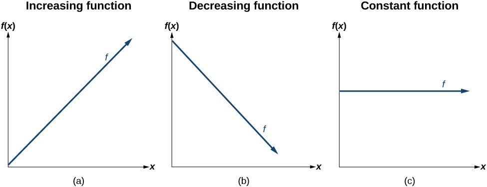
Figure 4
The linear functions we used in the two previous examples increased over time, but not every linear function does. A linear function may be increasing, decreasing, or constant.
For an increasing function, as with the train example,
the output values increase as the input values increase.
The graph of an increasing function has a positive slope. A line with a positive slope slants upward from left to right as in (a).
For a decreasing function, the slope is negative.
The output values decrease as the input values increase.
A line with a negative slope slants downward from left to right as in (b). If the function is constant, the output values are the same for all input values so the slope is zero. A line with a slope of zero is horizontal as in (c).
The slope determines if the function is an increasing linear function, a decreasing linear function, or a constant function.
Some recent studies suggest that a teenager sends an average of 60 texts per day. (http://www.cbsnews.com/8301-501465_162-57400228-501465/teens-are-sending-60-texts-a-day-study-says/) For each of the following scenarios, find the linear function that describes the relationship between the input value and the output value. Then, determine whether the graph of the function is increasing, decreasing, or constant.
Analyze each function.
In the examples we have seen so far, we have had the slope provided for us. However, we often need to calculate the slope given input and output values. Given two values for the input, [latex]{x}_{1}[/latex] and [latex]{x}_{2}[/latex], and two corresponding values for the output, [latex]{y}_{1}[/latex] and [latex]{y}_{2}[/latex] —which can be represented by a set of points, [latex]\left({x}_{1}\text{, }{y}_{1}\right)[/latex] and [latex]\left({x}_{2}\text{, }{y}_{2}\right)[/latex]—we can calculate the slope [latex]m[/latex], as follows
where [latex]\Delta y\\[/latex] is the vertical displacement and [latex]\Delta x\\[/latex] is the horizontal displacement. Note in function notation two corresponding values for the output [latex]{y}_{1}\\[/latex] and [latex]{y}_{2}\\[/latex] for the function [latex]f[/latex], [latex]{y}_{1}=f\left({x}_{1}\right)\\[/latex] and [latex]{y}_{2}=f\left({x}_{2}\right)\\[/latex], so we could equivalently write
The graph in Figure 5 indicates how the slope of the line between the points, [latex]\left({x}_{1,}{y}_{1}\right)\\[/latex]
and [latex]\left({x}_{2,}{y}_{2}\right)\\[/latex], is calculated. Recall that the slope measures steepness. The greater the absolute value of the slope, the steeper the line is.
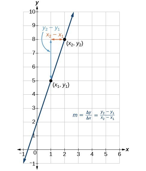
Figure 5
The slope of a function is calculated by the change in [latex]y[/latex] divided by the change in [latex]x[/latex]. It does not matter which coordinate is used as the [latex]\left({x}_{2,\text{ }}{y}_{2}\right)[/latex] and which is the [latex]\left({x}_{1},\text{ }{y}_{1}\right)[/latex], as long as each calculation is started with the elements from the same coordinate pair.
Are the units for slope always [latex]\frac{\text{units for the output}}{\text{units for the input}}\\[/latex] ?
Yes. Think of the units as the change of output value for each unit of change in input value. An example of slope could be miles per hour or dollars per day. Notice the units appear as a ratio of units for the output per units for the input.
The slope, or rate of change, of a function [latex]m[/latex] can be calculated according to the following:
where [latex]{x}_{1}\\[/latex] and [latex]{x}_{2}\\[/latex] are input values, [latex]{y}_{1}\\[/latex] and [latex]{y}_{2}\\[/latex] are output values.
If [latex]f\left(x\right)[/latex] is a linear function, and [latex]\left(3,-2\right)\\[/latex] and [latex]\left(8,1\right)\\[/latex] are points on the line, find the slope. Is this function increasing or decreasing?
The coordinate pairs are [latex]\left(3,-2\right)\\[/latex] and [latex]\left(8,1\right)\\[/latex]. To find the rate of change, we divide the change in output by the change in input.
We could also write the slope as [latex]m=0.6[/latex]. The function is increasing because [latex]m>0[/latex].
As noted earlier, the order in which we write the points does not matter when we compute the slope of the line as long as the first output value, or y-coordinate, used corresponds with the first input value, or x-coordinate, used.
If [latex]f\left(x\right)[/latex] is a linear function, and [latex]\left(2,\text{ }3\right)\\[/latex] and [latex]\left(0,\text{ }4\right)\\[/latex] are points on the line, find the slope. Is this function increasing or decreasing?
The population of a city increased from 23,400 to 27,800 between 2008 and 2012. Find the change of population per year if we assume the change was constant from 2008 to 2012.
The rate of change relates the change in population to the change in time. The population increased by [latex]27,800 - 23,400=4400[/latex] people over the four-year time interval. To find the rate of change, divide the change in the number of people by the number of years.
So the population increased by 1,100 people per year.
Because we are told that the population increased, we would expect the slope to be positive. This positive slope we calculated is therefore reasonable.
The population of a small town increased from 1,442 to 1,868 between 2009 and 2012. Find the change of population per year if we assume the change was constant from 2009 to 2012.
Up until now, we have been using the slope-intercept form of a linear equation to describe linear functions. Here, we will learn another way to write a linear function, the point-slope form.
The point-slope form is derived from the slope formula.
Keep in mind that the slope-intercept form and the point-slope form can be used to describe the same function. We can move from one form to another using basic algebra. For example, suppose we are given an equation in point-slope form, [latex]y - 4=-\frac{1}{2}\left(x - 6\right)\\[/latex] . We can convert it to the slope-intercept form as shown.
Therefore, the same line can be described in slope-intercept form as [latex]y=-\frac{1}{2}x+7\\[/latex].
The point-slope form of a linear equation takes the form
where [latex]m[/latex] is the slope, [latex]{x}_{1 }\text{and} {y}_{1}\\[/latex] are the [latex]x\text{ and }y\\[/latex] coordinates of a specific point through which the line passes.
The point-slope form is particularly useful if we know one point and the slope of a line. Suppose, for example, we are told that a line has a slope of 2 and passes through the point [latex]\left(4,1\right)\\[/latex]. We know that [latex]m=2\\[/latex] and that [latex]{x}_{1}=4\\[/latex] and [latex]{y}_{1}=1\\[/latex]. We can substitute these values into the general point-slope equation.
If we wanted to then rewrite the equation in slope-intercept form, we apply algebraic techniques.
Both equations, [latex]y - 1=2\left(x - 4\right)\\[/latex] and [latex]y=2x - 7\\[/latex], describe the same line. See Figure 6.
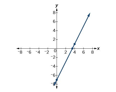
Figure 6
Write the point-slope form of an equation of a line with a slope of 3 that passes through the point [latex]\left(6,-1\right)\\[/latex]. Then rewrite it in the slope-intercept form.
Let’s figure out what we know from the given information. The slope is 3, so m = 3. We also know one point, so we know [latex]{x}_{1}=6\\[/latex] and [latex]{y}_{1}=-1\\[/latex]. Now we can substitute these values into the general point-slope equation.
Then we use algebra to find the slope-intercept form.
Write the point-slope form of an equation of a line with a slope of –2 that passes through the point [latex]\left(-2,\text{ }2\right)\\[/latex]. Then rewrite it in the slope-intercept form.
The point-slope form of an equation is also useful if we know any two points through which a line passes. Suppose, for example, we know that a line passes through the points [latex]\left(0,\text{ }1\right)\\[/latex] and [latex]\left(3,\text{ }2\right)\\[/latex]. We can use the coordinates of the two points to find the slope.
Now we can use the slope we found and the coordinates of one of the points to find the equation for the line. Let use (0, 1) for our point.
As before, we can use algebra to rewrite the equation in the slope-intercept form.
Both equations describe the line shown in Figure 7.
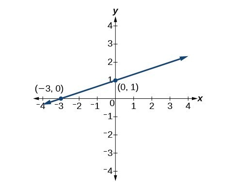
Figure 7
Write the point-slope form of an equation of a line that passes through the points (5, 1) and (8, 7). Then rewrite it in the slope-intercept form.
Let’s begin by finding the slope.
So [latex]m=2\\[/latex]. Next, we substitute the slope and the coordinates for one of the points into the general point-slope equation. We can choose either point, but we will use [latex]\left(5,1\right)\\[/latex].
The point-slope equation of the line is [latex]{y}_{2}-1=2\left({x}_{2}-5\right)\\[/latex]. To rewrite the equation in slope-intercept form, we use algebra.
The slope-intercept equation of the line is [latex]y=2x - 9\\[/latex].
Write the point-slope form of an equation of a line that passes through the points [latex]\left(-1,3\right)\\ [/latex] and [latex]\left(0,0\right)\\[/latex]. Then rewrite it in the slope-intercept form.
Now that we have written equations for linear functions in both the slope-intercept form and the point-slope form, we can choose which method to use based on the information we are given. That information may be provided in the form of a graph, a point and a slope, two points, and so on. Look at the graph of the function f in Figure 8.
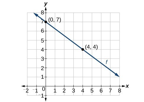
Figure 8
We are not given the slope of the line, but we can choose any two points on the line to find the slope. Let’s choose (0, 7) and (4, 4). We can use these points to calculate the slope.
Now we can substitute the slope and the coordinates of one of the points into the point-slope form.
If we want to rewrite the equation in the slope-intercept form, we would find

Figure 9
If we wanted to find the slope-intercept form without first writing the point-slope form, we could have recognized that the line crosses the y-axis when the output value is 7. Therefore, b = 7. We now have the initial value b and the slope m so we can substitute m and b into the slope-intercept form of a line.
So the function is [latex]f\left(x\right)=-\frac{3}{4}x+7\\[/latex], and the linear equation would be [latex]y=-\frac{3}{4}x+7\\[/latex].
Write an equation for a linear function given a graph of f shown in Figure 10.
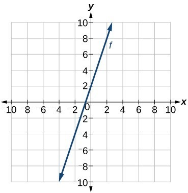
Figure 10
Identify two points on the line, such as (0, 2) and (–2, –4). Use the points to calculate the slope.
Substitute the slope and the coordinates of one of the points into the point-slope form.
We can use algebra to rewrite the equation in the slope-intercept form.
This makes sense because we can see from Figure 11 that the line crosses the y-axis at the point (0, 2), which is the y-intercept, so b = 2.
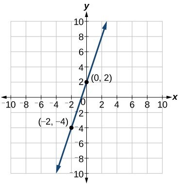
Figure 11
Suppose Ben starts a company in which he incurs a fixed cost of $1,250 per month for the overhead, which includes his office rent. His production costs are $37.50 per item. Write a linear function C where C(x) is the cost for x items produced in a given month.
The fixed cost is present every month, $1,250. The costs that can vary include the cost to produce each item, which is $37.50 for Ben. The variable cost, called the marginal cost, is represented by 37.5. The cost Ben incurs is the sum of these two costs, represented by [latex]C\left(x\right)=1250+37.5x\\[/latex].
If Ben produces 100 items in a month, his monthly cost is represented by
So his monthly cost would be $5,000.
If f is a linear function, with [latex]f\left(3\right)=-2\\[/latex] , and [latex]f\left(8\right)=1\\[/latex], find an equation for the function in slope-intercept form.
We can write the given points using coordinates.
We can then use the points to calculate the slope.
Substitute the slope and the coordinates of one of the points into the point-slope form.
We can use algebra to rewrite the equation in the slope-intercept form.
If [latex]f\left(x\right)\\[/latex] is a linear function, with [latex]f\left(2\right)=-11\\[/latex], and [latex]f\left(4\right)=-25\\[/latex], find an equation for the function in slope-intercept form.
In the real world, problems are not always explicitly stated in terms of a function or represented with a graph. Fortunately, we can analyze the problem by first representing it as a linear function and then interpreting the components of the function. As long as we know, or can figure out, the initial value and the rate of change of a linear function, we can solve many different kinds of real-world problems.
Marcus currently has 200 songs in his music collection. Every month, he adds 15 new songs. Write a formula for the number of songs, N, in his collection as a function of time, t, the number of months. How many songs will he own in a year?
The initial value for this function is 200 because he currently owns 200 songs, so N(0) = 200, which means that b = 200.

Figure 12
The number of songs increases by 15 songs per month, so the rate of change is 15 songs per month. Therefore we know that m = 15. We can substitute the initial value and the rate of change into the slope-intercept form of a line.
We can write the formula [latex]N\left(t\right)=15t+200\\[/latex].
With this formula, we can then predict how many songs Marcus will have in 1 year (12 months). In other words, we can evaluate the function at t = 12.
Marcus will have 380 songs in 12 months.
Notice that N is an increasing linear function. As the input (the number of months) increases, the output (number of songs) increases as well.
Working as an insurance salesperson, Ilya earns a base salary plus a commission on each new policy. Therefore, Ilya’s weekly income, I, depends on the number of new policies, n, he sells during the week. Last week he sold 3 new policies, and earned $760 for the week. The week before, he sold 5 new policies and earned $920. Find an equation for I(n), and interpret the meaning of the components of the equation.
The given information gives us two input-output pairs: (3, 760) and (5, 920). We start by finding the rate of change.
Keeping track of units can help us interpret this quantity. Income increased by $160 when the number of policies increased by 2, so the rate of change is $80 per policy. Therefore, Ilya earns a commission of $80 for each policy sold during the week.
We can then solve for the initial value.
The value of b is the starting value for the function and represents Ilya’s income when n = 0, or when no new policies are sold. We can interpret this as Ilya’s base salary for the week, which does not depend upon the number of policies sold.
We can now write the final equation.
Our final interpretation is that Ilya’s base salary is $520 per week and he earns an additional $80 commission for each policy sold.
The table below relates the number of rats in a population to time, in weeks. Use the table to write a linear equation.
| w, number of weeks | 0 | 2 | 4 | 6 |
| P(w), number of rats | 1000 | 1080 | 1160 | 1240 |
We can see from the table that the initial value for the number of rats is 1000, so b = 1000.
Rather than solving for m, we can tell from looking at the table that the population increases by 80 for every 2 weeks that pass. This means that the rate of change is 80 rats per 2 weeks, which can be simplified to 40 rats per week.
If we did not notice the rate of change from the table we could still solve for the slope using any two points from the table. For example, using (2, 1080) and (6, 1240)
Is the initial value always provided in a table of values like the table in Example 12?
No. Sometimes the initial value is provided in a table of values, but sometimes it is not. If you see an input of 0, then the initial value would be the corresponding output. If the initial value is not provided because there is no value of input on the table equal to 0, find the slope, substitute one coordinate pair and the slope into [latex]f\left(x\right)=mx+b\\[/latex], and solve for b.
A new plant food was introduced to a young tree to test its effect on the height of the tree. The table below shows the height of the tree, in feet, x months since the measurements began. Write a linear function, H(x), where x is the number of months since the start of the experiment.
| x | 0 | 2 | 4 | 8 | 12 |
| H(x) | 12.5 | 13.5 | 14.5 | 16.5 | 18.5 |
| slope-intercept form of a line | [latex]f\left(x\right)=mx+b\\[/latex] |
| slope | [latex]m=\frac{\text{change in output (rise)}}{\text{change in input (run)}}=\frac{\Delta y}{\Delta x}=\frac{{y}_{2}-{y}_{1}}{{x}_{2}-{x}_{1}}\\[/latex] |
| point-slope form of a line | [latex]y-{y}_{1}=m\left(x-{x}_{1}\right)\\[/latex] |
1. Terry is skiing down a steep hill. Terry’s elevation, E(t), in feet after t seconds is given by [latex]E\left(t\right)=3000-70t\\[/latex]. Write a complete sentence describing Terry’s starting elevation and how it is changing over time.
2. Maria is climbing a mountain. Maria’s elevation, E(t), in feet after t minutes is given by [latex]E\left(t\right)=1200+40t\\[/latex]. Write a complete sentence describing Maria’s starting elevation and how it is changing over time.
3. Jessica is walking home from a friend’s house. After 2 minutes she is 1.4 miles from home. Twelve minutes after leaving, she is 0.9 miles from home. What is her rate in miles per hour?
4. Sonya is currently 10 miles from home and is walking farther away at 2 miles per hour. Write an equation for her distance from home t hours from now.
5. A boat is 100 miles away from the marina, sailing directly toward it at 10 miles per hour. Write an equation for the distance of the boat from the marina after t hours.
6. Timmy goes to the fair with $40. Each ride costs $2. How much money will he have left after riding [latex]n[/latex] rides?
For the following exercises, determine whether the equation of the curve can be written as a linear function.
7. [latex]y=\frac{1}{4}x+6\\[/latex]
8. [latex]y=3x - 5\\[/latex]
9. [latex]y=3{x}^{2}-2\\[/latex]
10. [latex]3x+5y=15\\[/latex]
11. [latex]3{x}^{2}+5y=15\\[/latex]
12. [latex]3x+5{y}^{2}=15\\[/latex]
13. [latex]-2{x}^{2}+3{y}^{2}=6\\[/latex]
14. [latex]-\frac{x - 3}{5}=2y\\[/latex]
For the following exercises, determine whether each function is increasing or decreasing.
15. [latex]f\left(x\right)=4x+3\\[/latex]
16. [latex]g\left(x\right)=5x+6\\[/latex]
17. [latex]a\left(x\right)=5 - 2x\\[/latex]
18. [latex]b\left(x\right)=8 - 3x\\[/latex]
19. [latex]h\left(x\right)=-2x+4\\[/latex]
20. [latex]k\left(x\right)=-4x+1\\[/latex]
21. [latex]j\left(x\right)=\frac{1}{2}x - 3\\[/latex]
22. [latex]p\left(x\right)=\frac{1}{4}x - 5\\[/latex]
23. [latex]n\left(x\right)=-\frac{1}{3}x - 2\\[/latex]
24. [latex]m\left(x\right)=-\frac{3}{8}x+3\\[/latex]
For the following exercises, find the slope of the line that passes through the two given points.
25. [latex]\left(2,\text{ }4\right)\\[/latex] and [latex]\left(4,\text{ 10}\right)\\[/latex]
26. [latex]\left(1,\text{ 5}\right)\\[/latex] and [latex]\left(4,\text{ 11}\right)\\[/latex]
27. [latex]\left(-1,\text{4}\right)\\[/latex] and [latex]\left(5,\text{2}\right)\\[/latex]
28. [latex]\left(8,-2\right)\\[/latex] and [latex]\left(4,6\right)\\[/latex]
29. [latex]\left(6,\text{ }11\right)\\[/latex] and [latex]\left(-4, 3\right)\\[/latex]
For the following exercises, given each set of information, find a linear equation satisfying the conditions, if possible.
30. [latex]f\left(-5\right)=-4\\[/latex], and [latex]f\left(5\right)=2\\[/latex]
31. [latex]f\left(-1\right)=4\\[/latex] and [latex]f\left(5\right)=1\\[/latex]
32. [latex]\left(2,4\right)\\[/latex] and [latex]\left(4,10\right)\\[/latex]
33. Passes through [latex]\left(1,5\right)\\[/latex] and [latex]\left(4,11\right)\\[/latex]
34. Passes through [latex]\left(-1,\text{ 4}\right)\\[/latex] and [latex]\left(5,\text{ 2}\right)\\[/latex]
35. Passes through [latex]\left(-2,\text{ 8}\right)\\[/latex] and [latex]\left(4,\text{ 6}\right)\\[/latex]
36. x intercept at [latex]\left(-2,\text{ 0}\right)\\[/latex] and y intercept at [latex]\left(0,-3\right)\\[/latex]
37. x intercept at [latex]\left(-5,\text{ 0}\right)\\[/latex] and y intercept at [latex]\left(0,\text{ 4}\right)\\[/latex]
For the following exercises, find the slope of the lines graphed.
38.
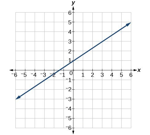
39.

40.
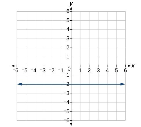
For the following exercises, write an equation for the lines graphed.
41.

42.
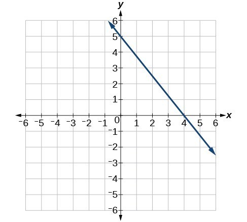
43.
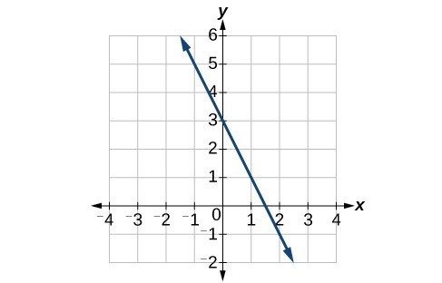
44.
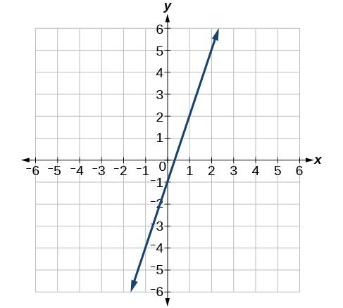
45.
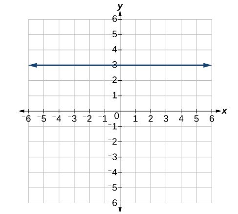
46.
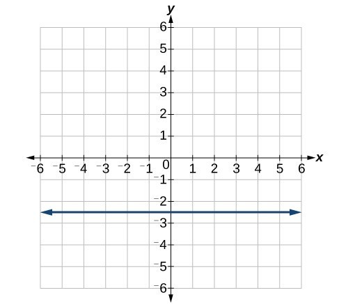
For the following exercises, which of the tables could represent a linear function? For each that could be linear, find a linear equation that models the data.
47.
| x | 0 | 5 | 10 | 15 |
| g(x) | 5 | –10 | –25 | –40 |
48.
| x | 0 | 5 | 10 | 15 |
| h(x) | 5 | 30 | 105 | 230 |
49.
| x | 0 | 5 | 10 | 15 |
| f(x) | –5 | 20 | 45 | 70 |
50.
| x | 5 | 10 | 20 | 25 |
| k(x) | 28 | 13 | 58 | 73 |
51.
| x | 0 | 2 | 4 | 6 |
| g(x) | 6 | –19 | –44 | –69 |
52.
| x | 2 | 4 | 6 | 8 |
| f(x) | –4 | 16 | 36 | 56 |
53.
| x | 2 | 4 | 6 | 8 |
| f(x) | –4 | 16 | 36 | 56 |
54.
| x | 0 | 2 | 6 | 8 |
| k(x) | 6 | 31 | 106 | 231 |
55. If f is a linear function, [latex]f\left(0.1\right)=11.5, \text{ and} f\left(0.4\right)=-5.9\\[/latex], find an equation for the function.
56. Graph the function f on a domain of [latex]\left[-10, 10\right]: f\left(x\right)=0.02x - 0.01\\[/latex]. Enter the function in a graphing utility. For the viewing window, set the minimum value of x to be –10 and the maximum value of x to be 10.
57. Graph the function f on a domain of [latex]\left[-10, 10\right]:f\left(x\right)=2,500x+4,000\\[/latex]
58. The table below shows the input, w, and output, k, for a linear function k. a. Fill in the missing values of the table. b. Write the linear function k, round to 3 decimal places.
| w | –10 | 5.5 | 67.5 | b |
| k | 30 | –26 | a | –44 |
59. shows the input, p, and output, q, for a linear function q. a. Fill in the missing values of the table. b. Write the linear function k.
| p | 0.5 | 0.8 | 12 | b |
| q | 400 | 700 | a | 1,000,000 |
60. Graph the linear function f on a domain of [–10, 10] for the function whose slope is [latex]\frac{1}{8}\\[/latex] and y-intercept is [latex]\frac{31}{16}\\[/latex]. Label the points for the input values of –10 and 10.
61. Graph the linear function f on a domain of [–0.1, 0.1] for the function whose slope is 75 and y-intercept is –22.5. Label the points for the input values of –0.1 and 0.1.
62. Graph the linear function f where [latex]f\left(x\right)=ax+b\\[/latex] on the same set of axes on a domain of [–4, 4] for the following values of a and b.
63. Find the value of x if a linear function goes through the following points and has the following slope: [latex]\left(x,2\right),\left(-4,6\right),m=3\\[/latex]
64. Find the value of y if a linear function goes through the following points and has the following slope: [latex]\left(10,y\right),\left(25,100\right),m=-5\\[/latex]
65. Find the equation of the line that passes through the following points: [latex]\left(a,\text{ }b\right)\\[/latex] and [latex]\left(a,\text{ }b+1\right)\\[/latex]
66. Find the equation of the line that passes through the following points: [latex]\left(2a,\text{ }b\right)\\[/latex] and [latex]\left(a,\text{ }b+1\right)\\[/latex]
67. Find the equation of the line that passes through the following points: [latex]\left(a,\text{ }0\right)\\[/latex] and [latex]\left(c,\text{ }d\right)\\[/latex]
68. At noon, a barista notices that she has $20 in her tip jar. If she makes an average of $0.50 from each customer, how much will she have in her tip jar if she serves n more customers during her shift?
69. A gym membership with two personal training sessions costs $125, while gym membership with five personal training sessions costs $260. What is cost per session?
70. A clothing business finds there is a linear relationship between the number of shirts, n, it can sell and the price, p, it can charge per shirt. In particular, historical data shows that 1,000 shirts can be sold at a price of $30, while 3,000 shirts can be sold at a price of $22. Find a linear equation in the form [latex]p\left(n\right)=mn+b\\[/latex] that gives the price p they can charge for n shirts.
71. A phone company charges for service according to the formula: [latex]C\left(n\right)=24+0.1n\\[/latex], where n is the number of minutes talked, and [latex]C\left(n\right)\\[/latex] is the monthly charge, in dollars. Find and interpret the rate of change and initial value.
72. A farmer finds there is a linear relationship between the number of bean stalks, n, she plants and the yield, y, each plant produces. When she plants 30 stalks, each plant yields 30 oz of beans. When she plants 34 stalks, each plant produces 28 oz of beans. Find a linear relationships in the form [latex]y=\mathrm{mn}+b\\[/latex] that gives the yield when n stalks are planted.
73. A city’s population in the year 1960 was 287,500. In 1989 the population was 275,900. Compute the rate of growth of the population and make a statement about the population rate of change in people per year.
74. A town’s population has been growing linearly. In 2003, the population was 45,000, and the population has been growing by 1,700 people each year. Write an equation, [latex]P\left(t\right)\\[/latex], for the population t years after 2003.
75. Suppose that average annual income (in dollars) for the years 1990 through 1999 is given by the linear function: [latex]I\left(x\right)=1054x+23,286\\[/latex], where x is the number of years after 1990. Which of the following interprets the slope in the context of the problem?
a. As of 1990, average annual income was $23,286.
b. In the ten-year period from 1990–1999, average annual income increased by a total of $1,054.
c. Each year in the decade of the 1990s, average annual income increased by $1,054.
d. Average annual income rose to a level of $23,286 by the end of 1999.
76. When temperature is 0 degrees Celsius, the Fahrenheit temperature is 32. When the Celsius temperature is 100, the corresponding Fahrenheit temperature is 212. Express the Fahrenheit temperature as a linear function of C, the Celsius temperature, [latex]F\left(C\right)\\[/latex].
a. Find the rate of change of Fahrenheit temperature for each unit change temperature of Celsius.
b. Find and interpret [latex]F\left(28\right)\\[/latex].
c. Find and interpret [latex]F\left(-40\right)\\[/latex].
1. [latex]m=\frac{4 - 3}{0 - 2}=\frac{1}{-2}=-\frac{1}{2}\\[/latex] ; decreasing because [latex]m<0\\[/latex].
2. [latex]m=\frac{1,868 - 1,442}{2,012 - 2,009}=\frac{426}{3}=142\text{ people per year}\\[/latex]
3. [latex]y - 2=-2\left(x+2\right)\\[/latex]; [latex]y=-2x - 2\\[/latex]
4. [latex]y - 0=-3\left(x - 0\right)\\[/latex] ; [latex]y=-3x\\[/latex]
5. [latex]y=-7x+3\\[/latex]
6. [latex]H\left(x\right)=0.5x+12.5\\[/latex]
1. Terry starts at an elevation of 3000 feet and descends 70 feet per second.
3. 3 miles per hour
5. [latex]d\left(t\right)=100 - 10t\\[/latex]
7. Yes.
9. No.
11. No.
13. No.
15. Increasing.
17. Decreasing.
19. Decreasing.
21. Increasing.
23. Decreasing.
25. 3
27. [latex]-\frac{1}{3}\\[/latex]
29. [latex]\frac{4}{5}\\[/latex]
31. [latex]f\left(x\right)=-\frac{1}{2}x+\frac{7}{2}\\[/latex]
33. [latex]y=2x+3\\[/latex]
35. [latex]y=-\frac{1}{3}x+\frac{22}{3}\\[/latex]
37. [latex]y=\frac{4}{5}x+4\\[/latex]
39. [latex]-\frac{5}{4}\\[/latex]
41. [latex]y=\frac{2}{3}x+1\\[/latex]
43. [latex]y=-2x+3\\[/latex]
45. [latex]y=3\\[/latex]
47. Linear, [latex]g\left(x\right)=-3x+5\\[/latex]
49. Linear, [latex]f\left(x\right)=5x - 5\\[/latex]
51. Linear, [latex]g\left(x\right)=-\frac{25}{2}x+6\\[/latex]
53. Linear, [latex]f\left(x\right)=10x - 24\\[/latex]
55. [latex]f\left(x\right)=-58x+17.3\\[/latex]
57.

59. a. [latex]a=11,900\\[/latex] ; [latex]b=1001.1\\[/latex] b. [latex]q\left(p\right)=1000p - 100\\[/latex]
61.

63. [latex]x=-\frac{16}{3}\\[/latex]
65. [latex]x=a\\[/latex]
67. [latex]y=\frac{d}{c-a}x-\frac{ad}{c-a}\\[/latex]
69. $45 per training session.
71. The rate of change is 0.1. For every additional minute talked, the monthly charge increases by $0.1 or 10 cents. The initial value is 24. When there are no minutes talked, initially the charge is $24.
73. The slope is –400. This means for every year between 1960 and 1989, the population dropped by 400 per year in the city.
75. c
By the end of this lesson, you will be able to:
Two competing telephone companies offer different payment plans. The two plans charge the same rate per long distance minute, but charge a different monthly flat fee. A consumer wants to determine whether the two plans will ever cost the same amount for a given number of long distance minutes used. The total cost of each payment plan can be represented by a linear function. To solve the problem, we will need to compare the functions. In this section, we will consider methods of comparing functions using graphs.
In Linear Functions, we saw that that the graph of a linear function is a straight line. We were also able to see the points of the function as well as the initial value from a graph. By graphing two functions, then, we can more easily compare their characteristics.
There are three basic methods of graphing linear functions. The first is by plotting points and then drawing a line through the points. The second is by using the y-intercept and slope. And the third is by using transformations of the identity function [latex]f\left(x\right)=x\\[/latex].
To find points of a function, we can choose input values, evaluate the function at these input values, and calculate output values. The input values and corresponding output values form coordinate pairs. We then plot the coordinate pairs on a grid. In general, we should evaluate the function at a minimum of two inputs in order to find at least two points on the graph. For example, given the function, [latex]f\left(x\right)=2x\\[/latex], we might use the input values 1 and 2. Evaluating the function for an input value of 1 yields an output value of 2, which is represented by the point (1, 2). Evaluating the function for an input value of 2 yields an output value of 4, which is represented by the point (2, 4). Choosing three points is often advisable because if all three points do not fall on the same line, we know we made an error.
Graph [latex]f\left(x\right)=-\frac{2}{3}x+5\\[/latex] by plotting points.
Begin by choosing input values. This function includes a fraction with a denominator of 3, so let’s choose multiples of 3 as input values. We will choose 0, 3, and 6.
Evaluate the function at each input value, and use the output value to identify coordinate pairs.
Plot the coordinate pairs and draw a line through the points. Figure 1 shows the graph of the function [latex]f\left(x\right)=-\frac{2}{3}x+5\\[/latex].
![The graph of the linear function [latex]f\left(x\right)=-\frac{2}{3}x+5[/latex].](https://s3-us-west-2.amazonaws.com/courses-images-archive-read-only/wp-content/uploads/sites/924/2015/11/25201047/CNX_Precalc_Figure_02_02_0012.jpg)
Figure 1
The graph of the function is a line as expected for a linear function. In addition, the graph has a downward slant, which indicates a negative slope. This is also expected from the negative constant rate of change in the equation for the function.
Another way to graph linear functions is by using specific characteristics of the function rather than plotting points. The first characteristic is its y-intercept, which is the point at which the input value is zero. To find the y-intercept, we can set x = 0 in the equation.
The other characteristic of the linear function is its slope m, which is a measure of its steepness. Recall that the slope is the rate of change of the function. The slope of a function is equal to the ratio of the change in outputs to the change in inputs. Another way to think about the slope is by dividing the vertical difference, or rise, by the horizontal difference, or run. We encountered both the y-intercept and the slope in Linear Functions.
Let’s consider the following function.
[latex]f\left(x\right)=\frac{1}{2}x+1\\[/latex]
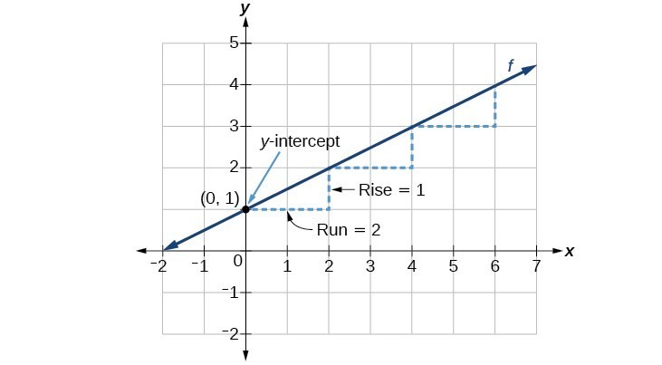
Figure 2
In the equation [latex]f\left(x\right)=mx+b\\[/latex]
Do all linear functions have y-intercepts?
Yes. All linear functions cross the y-axis and therefore have y-intercepts. (Note: A vertical line parallel to the y-axis does not have a y-intercept, but it is not a function.)
Graph [latex]f\left(x\right)=-\frac{2}{3}x+5\\[/latex] using the y-intercept and slope.
Evaluate the function at x = 0 to find the y-intercept. The output value when x = 0 is 5, so the graph will cross the y-axis at (0, 5).
According to the equation for the function, the slope of the line is [latex]-\frac{2}{3}\\[/latex]. This tells us that for each vertical decrease in the “rise” of –2 units, the “run” increases by 3 units in the horizontal direction. We can now graph the function by first plotting the y-intercept in Figure 3. From the initial value (0, 5) we move down 2 units and to the right 3 units. We can extend the line to the left and right by repeating, and then draw a line through the points.
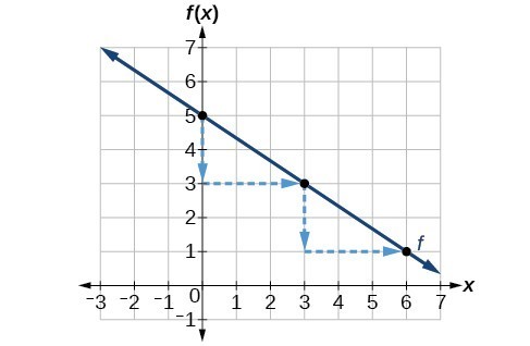
Figure 3
The graph slants downward from left to right, which means it has a negative slope as expected.
Another option for graphing is to use transformations of the identity function [latex]f\left(x\right)=x\\[/latex] . A function may be transformed by a shift up, down, left, or right. A function may also be transformed using a reflection, stretch, or compression.
In the equation [latex]f\left(x\right)=mx\\[/latex], the m is acting as the vertical stretch or compression of the identity function. When m is negative, there is also a vertical reflection of the graph. Notice in Figure 4 that multiplying the equation of [latex]f\left(x\right)=x\\[/latex] by m stretches the graph of f by a factor of m units if m > 1 and compresses the graph of f by a factor of m units if 0 < m < 1. This means the larger the absolute value of m, the steeper the slope.
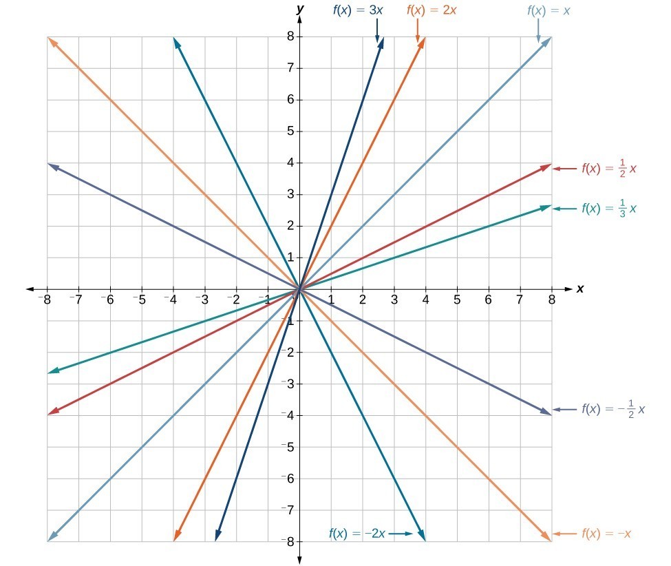
Figure 4. Vertical stretches and compressions and reflections on the function [latex]f\left(x\right)=x\\[/latex].
In [latex]f\left(x\right)=mx+b\\[/latex], the b acts as the vertical shift, moving the graph up and down without affecting the slope of the line. Notice in Figure 5 that adding a value of b to the equation of [latex]f\left(x\right)=x\\[/latex] shifts the graph of f a total of b units up if b is positive and |b| units down if b is negative.
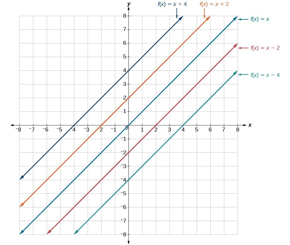
Figure 5. This graph illustrates vertical shifts of the function [latex]f\left(x\right)=x\\[/latex].
Using vertical stretches or compressions along with vertical shifts is another way to look at identifying different types of linear functions. Although this may not be the easiest way to graph this type of function, it is still important to practice each method.
Graph [latex]f\left(x\right)=\frac{1}{2}x - 3\\[/latex] using transformations.
The equation for the function shows that [latex]m=\frac{1}{2}\\[/latex] so the identity function is vertically compressed by [latex]\frac{1}{2}\\[/latex]. The equation for the function also shows that b = –3 so the identity function is vertically shifted down 3 units. First, graph the identity function, and show the vertical compression.
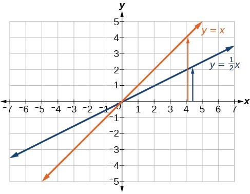
Figure 6. The function, y = x, compressed by a factor of [latex]\frac{1}{2}\\[/latex].
Then show the vertical shift.
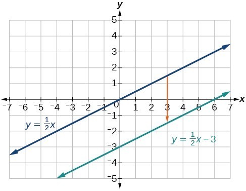
Figure 7. The function [latex]y=\frac{1}{2}x\\[/latex], shifted down 3 units.
In Example 3, could we have sketched the graph by reversing the order of the transformations?
No. The order of the transformations follows the order of operations. When the function is evaluated at a given input, the corresponding output is calculated by following the order of operations. This is why we performed the compression first. For example, following the order: Let the input be 2.
Recall that in Linear Functions, we wrote the equation for a linear function from a graph. Now we can extend what we know about graphing linear functions to analyze graphs a little more closely. Begin by taking a look at Figure 8. We can see right away that the graph crosses the y-axis at the point (0, 4) so this is the y-intercept.
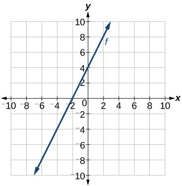
Figure 8
Then we can calculate the slope by finding the rise and run. We can choose any two points, but let’s look at the point (–2, 0). To get from this point to the y-intercept, we must move up 4 units (rise) and to the right 2 units (run). So the slope must be
Substituting the slope and y-intercept into the slope-intercept form of a line gives
Match each equation of the linear functions with one of the lines in Figure 9.
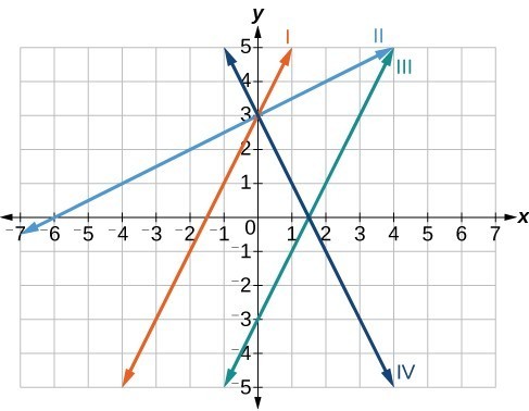
Figure 9
Analyze the information for each function.
Now we can re-label the lines as in Figure 10.
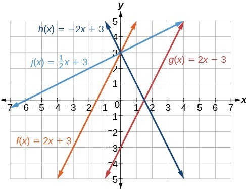
Figure 10
So far, we have been finding the y-intercepts of a function: the point at which the graph of the function crosses the y-axis. A function may also have an x-intercept, which is the x-coordinate of the point where the graph of the function crosses the x-axis. In other words, it is the input value when the output value is zero.
To find the x-intercept, set a function f(x) equal to zero and solve for the value of x. For example, consider the function shown.
Set the function equal to 0 and solve for x.
The graph of the function crosses the x-axis at the point (2, 0).
Do all linear functions have x-intercepts?
No. However, linear functions of the form y = c, where c is a nonzero real number are the only examples of linear functions with no x-intercept. For example, y = 5 is a horizontal line 5 units above the x-axis. This function has no x-intercepts.
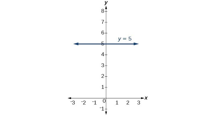
Figure 11
The x-intercept of the function is value of x when f(x) = 0. It can be solved by the equation 0 = mx + b.
Find the x-intercept of [latex]f\left(x\right)=\frac{1}{2}x - 3\\[/latex].
Set the function equal to zero to solve for x.
The graph crosses the x-axis at the point (6, 0).
A graph of the function is shown in Figure 12. We can see that the x-intercept is (6, 0) as we expected.
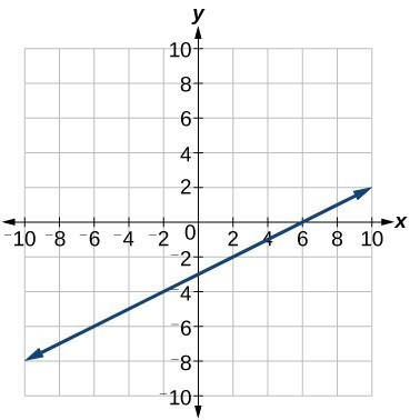
Figure 12. The graph of the linear function [latex]f\left(x\right)=\frac{1}{2}x - 3\\[/latex].
There are two special cases of lines on a graph—horizontal and vertical lines. A horizontal line indicates a constant output, or y-value. In Figure 13, we see that the output has a value of 2 for every input value. The change in outputs between any two points, therefore, is 0. In the slope formula, the numerator is 0, so the slope is 0. If we use m = 0 in the equation [latex]f\left(x\right)=mx+b\\[/latex], the equation simplifies to [latex]f\left(x\right)=b\\[/latex]. In other words, the value of the function is a constant. This graph represents the function [latex]f\left(x\right)=2\\[/latex].
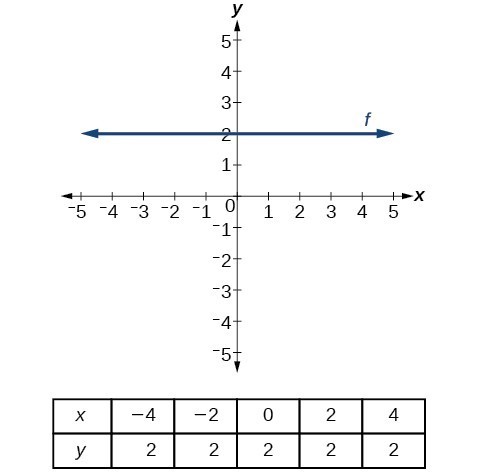
Figure 13. A horizontal line representing the function [latex]f\left(x\right)=2\\[/latex].
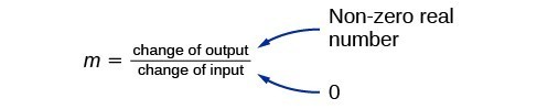
Figure 14
A vertical line indicates a constant input, or x-value. We can see that the input value for every point on the line is 2, but the output value varies. Because this input value is mapped to more than one output value, a vertical line does not represent a function. Notice that between any two points, the change in the input values is zero. In the slope formula, the denominator will be zero, so the slope of a vertical line is undefined.
Notice that a vertical line, such as the one in Figure 15, has an x-intercept, but no y-intercept unless it’s the line x = 0. This graph represents the line x = 2.
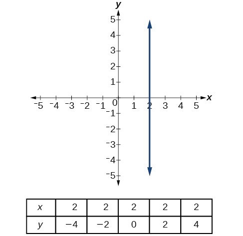
Figure 15. The vertical line, x = 2, which does not represent a function.
Lines can be horizontal or vertical.
A horizontal line is a line defined by an equation in the form [latex]f\left(x\right)=b\\[/latex].
A vertical line is a line defined by an equation in the form [latex]x=a\\[/latex].
Write the equation of the line graphed in Figure 16.
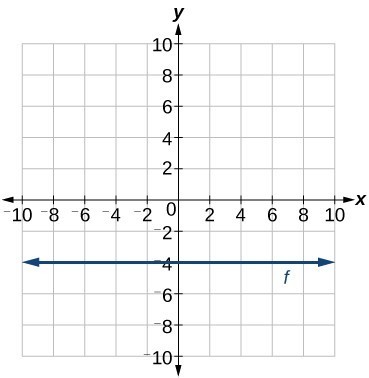
Figure 16
For any x-value, the y-value is –4, so the equation is y = –4.
Write the equation of the line graphed in Figure 17.
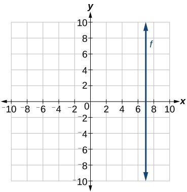
Figure 17
The constant x-value is 7, so the equation is x = 7.
The two lines in Figure 18 are parallel lines: they will never intersect. Notice that they have exactly the same steepness, which means their slopes are identical. The only difference between the two lines is the y-intercept. If we shifted one line vertically toward the y-intercept of the other, they would become the same line.
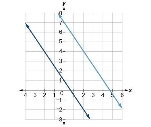
Figure 18. Parallel lines.
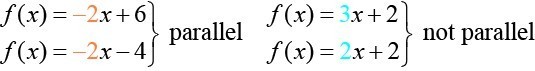
Figure 19.
We can determine from their equations whether two lines are parallel by comparing their slopes. If the slopes are the same and the y-intercepts are different, the lines are parallel. If the slopes are different, the lines are not parallel.
Unlike parallel lines, perpendicular lines do intersect. Their intersection forms a right, or 90-degree, angle. The two lines in Figure 20 are perpendicular.
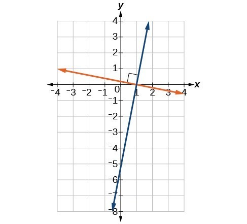
Figure 20. Perpendicular lines.
Perpendicular lines do not have the same slope. The slopes of perpendicular lines are different from one another in a specific way. The slope of one line is the negative reciprocal of the slope of the other line. The product of a number and its reciprocal is 1. So, if [latex]{m}_{1}\text{ and }{m}_{2}\\[/latex] are negative reciprocals of one another, they can be multiplied together to yield [latex]-1[/latex].
To find the reciprocal of a number, divide 1 by the number. So the reciprocal of 8 is [latex]\frac{1}{8}\\[/latex], and the reciprocal of [latex]\frac{1}{8}\\[/latex] is 8. To find the negative reciprocal, first find the reciprocal and then change the sign.
As with parallel lines, we can determine whether two lines are perpendicular by comparing their slopes, assuming that the lines are neither horizontal nor perpendicular. The slope of each line below is the negative reciprocal of the other so the lines are perpendicular.
The product of the slopes is –1.
Two lines are parallel lines if they do not intersect. The slopes of the lines are the same.
If and only if [latex]{b}_{1}={b}_{2}\\[/latex] and [latex]{m}_{1}={m}_{2}\\[/latex], we say the lines coincide. Coincident lines are the same line.
Two lines are perpendicular lines if they intersect at right angles.
Given the functions below, identify the functions whose graphs are a pair of parallel lines and a pair of perpendicular lines.
Parallel lines have the same slope. Because the functions [latex]f\left(x\right)=2x+3\\[/latex] and [latex]j\left(x\right)=2x - 6\\[/latex] each have a slope of 2, they represent parallel lines. Perpendicular lines have negative reciprocal slopes. Because −2 and [latex]\frac{1}{2}\\[/latex] are negative reciprocals, the equations, [latex]g\left(x\right)=\frac{1}{2}x - 4\\[/latex] and [latex]h\left(x\right)=-2x+2\\[/latex] represent perpendicular lines.
A graph of the lines is shown in Figure 21.
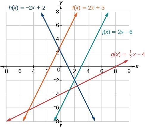
Figure 21. The graph shows that the lines [latex]f\left(x\right)=2x+3\\[/latex] and [latex]j\left(x\right)=2x - 6\\[/latex] are parallel, and the lines [latex]g\left(x\right)=\frac{1}{2}x - 4\\[/latex] and [latex]h\left(x\right)=-2x+2\\[/latex] are perpendicular.
If we know the equation of a line, we can use what we know about slope to write the equation of a line that is either parallel or perpendicular to the given line.
Suppose for example, we are given the following equation.
We know that the slope of the line formed by the function is 3. We also know that the y-intercept is (0, 1). Any other line with a slope of 3 will be parallel to f(x). So the lines formed by all of the following functions will be parallel to f(x).
Suppose then we want to write the equation of a line that is parallel to f and passes through the point (1, 7). We already know that the slope is 3. We just need to determine which value for b will give the correct line. We can begin with the point-slope form of an equation for a line, and then rewrite it in the slope-intercept form.
So [latex]g\left(x\right)=3x+4\\[/latex] is parallel to [latex]f\left(x\right)=3x+1\\[/latex] and passes through the point (1, 7).
Find a line parallel to the graph of [latex]f\left(x\right)=3x+6\\[/latex] that passes through the point (3, 0).
The slope of the given line is 3. If we choose the slope-intercept form, we can substitute m = 3, x = 3, and f(x) = 0 into the slope-intercept form to find the y-intercept.
The line parallel to f(x) that passes through (3, 0) is [latex]g\left(x\right)=3x - 9\\[/latex].
We can confirm that the two lines are parallel by graphing them. Figure 22 shows that the two lines will never intersect.
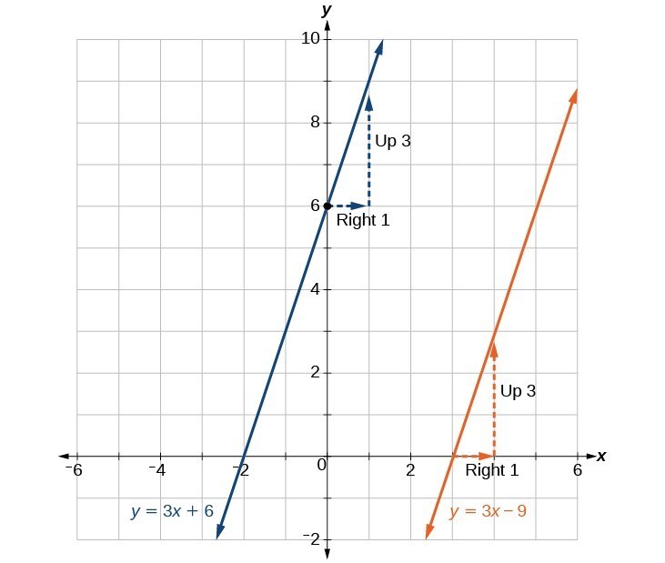
Figure 22
We can use a very similar process to write the equation for a line perpendicular to a given line. Instead of using the same slope, however, we use the negative reciprocal of the given slope. Suppose we are given the following function:
The slope of the line is 2, and its negative reciprocal is [latex]-\frac{1}{2}\\[/latex]. Any function with a slope of [latex]-\frac{1}{2}\\[/latex] will be perpendicular to f(x). So the lines formed by all of the following functions will be perpendicular to f(x).
As before, we can narrow down our choices for a particular perpendicular line if we know that it passes through a given point. Suppose then we want to write the equation of a line that is perpendicular to f(x) and passes through the point (4, 0). We already know that the slope is [latex]-\frac{1}{2}\\[/latex]. Now we can use the point to find the y-intercept by substituting the given values into the slope-intercept form of a line and solving for b.
The equation for the function with a slope of [latex]-\frac{1}{2}\\[/latex] and a y-intercept of 2 is
So [latex]g\left(x\right)=-\frac{1}{2}x+2\\[/latex] is perpendicular to [latex]f\left(x\right)=2x+4\\[/latex] and passes through the point (4, 0). Be aware that perpendicular lines may not look obviously perpendicular on a graphing calculator unless we use the square zoom feature.
A horizontal line has a slope of zero and a vertical line has an undefined slope. These two lines are perpendicular, but the product of their slopes is not –1. Doesn’t this fact contradict the definition of perpendicular lines?
No. For two perpendicular linear functions, the product of their slopes is –1. However, a vertical line is not a function so the definition is not contradicted.
Find the equation of a line perpendicular to [latex]f\left(x\right)=3x+3\\[/latex] that passes through the point (3, 0).
The original line has slope m = 3, so the slope of the perpendicular line will be its negative reciprocal, or [latex]-\frac{1}{3}\\[/latex]. Using this slope and the given point, we can find the equation for the line.
The line perpendicular to f(x) that passes through (3, 0) is [latex]g\left(x\right)=-\frac{1}{3}x+1\\[/latex].
A graph of the two lines is shown in Figure 23.
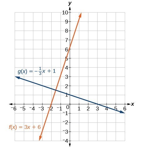
Figure 23
Given the function [latex]h\left(x\right)=2x - 4\\[/latex], write an equation for the line passing through (0, 0) that is
a. parallel to h(x)
b. perpendicular to h(x)
A line passes through the points (–2, 6) and (4, 5). Find the equation of a perpendicular line that passes through the point (4, 5).
From the two points of the given line, we can calculate the slope of that line.
Find the negative reciprocal of the slope.
We can then solve for the y-intercept of the line passing through the point (4, 5).
The equation for the line that is perpendicular to the line passing through the two given points and also passes through point (4, 5) is
A line passes through the points, (–2, –15) and (2, –3). Find the equation of a perpendicular line that passes through the point, (6, 4).
A system of linear equations includes two or more linear equations. The graphs of two lines will intersect at a single point if they are not parallel. Two parallel lines can also intersect if they are coincident, which means they are the same line and they intersect at every point. For two lines that are not parallel, the single point of intersection will satisfy both equations and therefore represent the solution to the system.
To find this point when the equations are given as functions, we can solve for an input value so that [latex]f\left(x\right)=g\left(x\right)\\[/latex]. In other words, we can set the formulas for the lines equal to one another, and solve for the input that satisfies the equation.
Find the point of intersection of the lines [latex]h\left(t\right)=3t - 4\\[/latex] and [latex]j\left(t\right)=5-t\\[/latex].
Set [latex]h\left(t\right)=j\left(t\right)\\[/latex].
This tells us the lines intersect when the input is [latex]\frac{9}{4}\\[/latex].
We can then find the output value of the intersection point by evaluating either function at this input.
These lines intersect at the point [latex]\left(\frac{9}{4},\frac{11}{4}\right)\\[/latex].
Looking at Figure 24, this result seems reasonable.
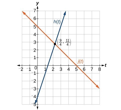
Figure 24
If we were asked to find the point of intersection of two distinct parallel lines, should something in the solution process alert us to the fact that there are no solutions?
Yes. After setting the two equations equal to one another, the result would be the contradiction “0 = non-zero real number”.
Using the graph in the Analysis of the Solution for Example 12, identify the following for the function [latex]j\left(t\right)\\[/latex]:
a. y-intercept
b. x-intercept(s)
c. slope
d. Is [latex]j\left(t\right)\\[/latex] parallel or perpendicular to [latex]h\left(t\right)\\[/latex] (or neither)?
e. Is [latex]j\left(t\right)\\[/latex] an increasing or decreasing function (or neither)?
f. Write a transformation description for [latex]j\left(t\right)\\[/latex] from the identity toolkit function [latex]f\left(x\right)=x\\[/latex].
A company sells sports helmets. The company incurs a one-time fixed cost for $250,000. Each helmet costs $120 to produce, and sells for $140.
To find [latex]y[/latex], evaluate either the revenue or the cost function at 12,500.
The break-even point is (12,500, 1,750,000).
This means if the company sells 12,500 helmets, they break even; both the sales and cost incurred equaled 1.75 million dollars.
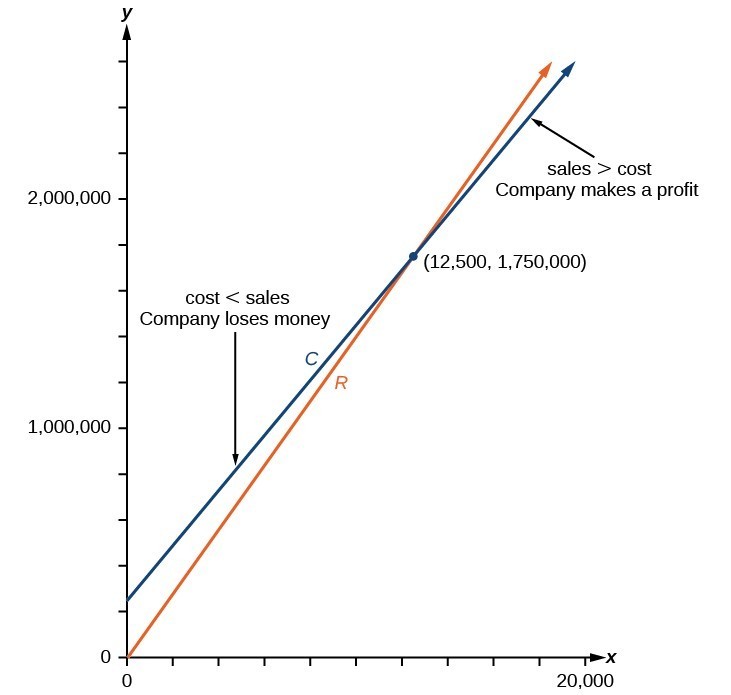
Figure 25
1. If the graphs of two linear functions are parallel, describe the relationship between the slopes and the y-intercepts.
2. If the graphs of two linear functions are perpendicular, describe the relationship between the slopes and the y-intercepts.
3. If a horizontal line has the equation [latex]f\left(x\right)=a\\[/latex] and a vertical line has the equation [latex]x=a\\[/latex], what is the point of intersection? Explain why what you found is the point of intersection.
4. Explain how to find a line parallel to a linear function that passes through a given point.
5. Explain how to find a line perpendicular to a linear function that passes through a given point.
For the following exercises, determine whether the lines given by the equations below are parallel, perpendicular, or neither parallel nor perpendicular:
6. [latex]\begin{cases}4x - 7y=10\hfill \\ 7x+4y=1\hfill \end{cases}\\[/latex]
7. [latex]\begin{cases}3y+x=12\\ -y=8x+1\end{cases}\\[/latex]
8. [latex]\begin{cases}3y+4x=12\\ -6y=8x+1\end{cases}\\[/latex]
9. [latex]\begin{cases}6x - 9y=10\\ 3x+2y=1\end{cases}\\[/latex]
10. [latex]\begin{cases}y=\frac{2}{3}x+1\\ 3x+2y=1\end{cases}\\[/latex]
11. [latex]\begin{cases}y=\frac{3}{4}x+1\\ -3x+4y=1\end{cases}\\[/latex]
For the following exercises, find the x- and y-intercepts of each equation.
12. [latex]f\left(x\right)=-x+2\\[/latex]
13. [latex]g\left(x\right)=2x+4\\[/latex]
14. [latex]h\left(x\right)=3x - 5\\[/latex]
15. [latex]k\left(x\right)=-5x+1\\[/latex]
16. [latex]-2x+5y=20\\[/latex]
17. [latex]7x+2y=56\\[/latex]
For the following exercises, use the descriptions of each pair of lines given below to find the slopes of Line 1 and Line 2. Is each pair of lines parallel, perpendicular, or neither?
18. Line 1: Passes through [latex]\left(0,6\right)\\[/latex] and [latex]\left(3,-24\right)\\[/latex]
Line 2: Passes through [latex]\left(-1,19\right)\\[/latex] and [latex]\left(8,-71\right)\\[/latex]
19. Line 1: Passes through [latex]\left(-8,-55\right)\\[/latex] and [latex]\left(10,89\right)\\[/latex]
Line 2: Passes through [latex]\left(9,-44\right)\\[/latex] and [latex]\left(4,-14\right)\\[/latex]
20. Line 1: Passes through [latex]\left(2,3\right)\\[/latex] and [latex]\left(4,-1\right)\\[/latex]
Line 2: Passes through [latex]\left(6,3\right)\\[/latex] and [latex]\left(8,5\right)\\[/latex]
21. Line 1: Passes through [latex]\left(1,7\right)\\[/latex] and [latex]\left(5,5\right)\\[/latex]
Line 2: Passes through [latex]\left(-1,-3\right)\\[/latex] and [latex]\left(1,1\right)\\[/latex]
22. Line 1: Passes through [latex]\left(0,5\right)\\[/latex] and [latex]\left(3,3\right)\\[/latex]
Line 2: Passes through [latex]\left(1,-5\right)\\[/latex] and [latex]\left(3,-2\right)\\[/latex]
23. Line 1: Passes through [latex]\left(2,5\right)\\[/latex] and [latex]\left(5,-1\right)\\[/latex]
Line 2: Passes through [latex]\left(-3,7\right)\\[/latex] and [latex]\left(3,-5\right)\\[/latex]
24. Write an equation for a line parallel to [latex]f\left(x\right)=-5x - 3\\[/latex] and passing through the point [latex]\left(2,\text{ -}12\right)\\[/latex].
25. Write an equation for a line parallel to [latex]g\left(x\right)=3x - 1\\[/latex] and passing through the point [latex]\left(4,9\right)\\[/latex].
26. Write an equation for a line perpendicular to [latex]h\left(t\right)=-2t+4\\[/latex] and passing through the point [latex]\left(\text{-}4,\text{ -}1\right)\\[/latex].
27. Write an equation for a line perpendicular to [latex]p\left(t\right)=3t+4\\[/latex] and passing through the point [latex]\left(3,1\right)\\[/latex].
28. Find the point at which the line [latex]f\left(x\right)=-2x - 1\\[/latex] intersects the line [latex]g\left(x\right)=-x\\[/latex].
29. Find the point at which the line [latex]f\left(x\right)=2x+5\\[/latex] intersects the line [latex]g\left(x\right)=-3x - 5\\[/latex].
30. Use algebra to find the point at which the line [latex]f\left(x\right)= -\frac{4}{5}x +\frac{274}{25}\\[/latex] intersects the line [latex]h\left(x\right)=\frac{9}{4}x+\frac{73}{10}\\[/latex].
31. Use algebra to find the point at which the line [latex]f\left(x\right)=\frac{7}{4}x+\frac{457}{60}\\[/latex] intersects the line [latex]g\left(x\right)=\frac{4}{3}x+\frac{31}{5}\\[/latex].
For the following exercises, the given linear equation with its graph.
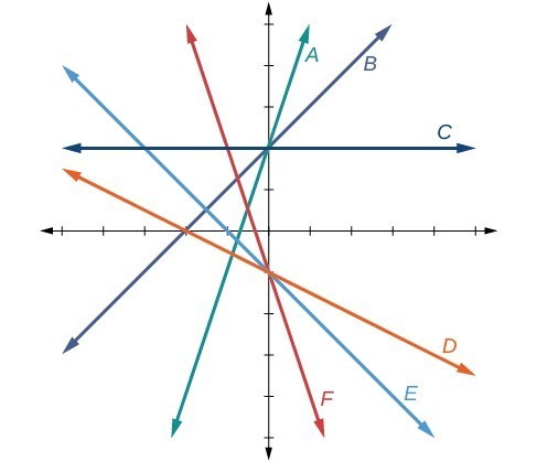
32. [latex]f\left(x\right)=-x - 1\\[/latex]
33. [latex]f\left(x\right)=-2x - 1\\[/latex]
34. [latex]f\left(x\right)=-\frac{1}{2}x - 1\\[/latex]
35. [latex]f\left(x\right)=2\\[/latex]
36. [latex]f\left(x\right)=2+x\\[/latex]
37. [latex]f\left(x\right)=3x+2\\[/latex]
For the following exercises, sketch a line with the given features.
38. An x-intercept of [latex]\left(-\text{4},\text{ 0}\right)\\[/latex] and y-intercept of [latex]\left(0,\text{ -2}\right)\\[/latex]
39. An x-intercept of [latex]\left(-\text{2},\text{ 0}\right)\\[/latex] and y-intercept of [latex]\left(0,\text{ 4}\right)\\[/latex]
40. A y-intercept of [latex]\left(0,\text{ 7}\right)\\[/latex] and slope [latex]-\frac{3}{2}\\[/latex]
41. A y-intercept of [latex]\left(0,\text{ 3}\right)\\[/latex] and slope [latex]\frac{2}{5}\\[/latex]
42. Passing through the points [latex]\left(-\text{6},\text{ -2}\right)\\[/latex] and [latex]\left(\text{6},\text{ -6}\right)\\[/latex]
43. Passing through the points [latex]\left(-\text{3},\text{ -4}\right)\\[/latex] and [latex]\left(\text{3},\text{ 0}\right)\\[/latex]
For the following exercises, sketch the graph of each equation.
44. [latex]f\left(x\right)=-2x - 1\\[/latex]
45. [latex]g\left(x\right)=-3x+2\\[/latex]
46. [latex]h\left(x\right)=\frac{1}{3}x+2\\[/latex]
47. [latex]k\left(x\right)=\frac{2}{3}x - 3\\[/latex]
48. [latex]f\left(t\right)=3+2t\\[/latex]
49. [latex]p\left(t\right)=-2+3t\\[/latex]
50. [latex]x=3\\[/latex]
51. [latex]x=-2\\[/latex]
52. [latex]r\left(x\right)=4\\[/latex]
53. [latex]q\left(x\right)=3\\[/latex]
54. [latex]4x=-9y+36\\[/latex]
55. [latex]\frac{x}{3}-\frac{y}{4}=1\\[/latex]
56. [latex]3x - 5y=15\\[/latex]
57. [latex]3x=15\\[/latex]
58. [latex]3y=12\\[/latex]
59. If [latex]g\left(x\right)\\[/latex] is the transformation of [latex]f\left(x\right)=x\\[/latex] after a vertical compression by [latex]\frac{3}{4}\\[/latex], a shift right by 2, and a shift down by 4
a. Write an equation for [latex]g\left(x\right)\\[/latex].
b. What is the slope of this line?
c. Find the y-intercept of this line.
60. If [latex]g\left(x\right)\\[/latex] is the transformation of [latex]f\left(x\right)=x\\[/latex] after a vertical compression by [latex]\frac{1}{3}\\[/latex], a shift left by 1, and a shift up by 3
a. Write an equation for [latex]g\left(x\right)\\[/latex].
b. What is the slope of this line?
c. Find the y-intercept of this line.
For the following exercises, write the equation of the line shown in the graph.
61.
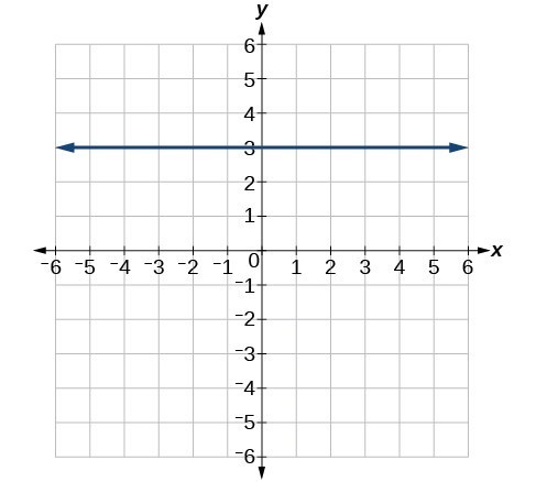
62.
63.
64.
For the following exercises, find the point of intersection of each pair of lines if it exists. If it does not exist, indicate that there is no point of intersection.
65. [latex]\begin{cases}y=\frac{3}{4}x+1\\ -3x+4y=12\end{cases}\\[/latex]
66. [latex]\begin{cases}2x - 3y=12\\ 5y+x=30\end{cases}\\[/latex]
67. [latex]\begin{cases}2x=y - 3\\ y+4x=15\end{cases}\\[/latex]
68. [latex]\begin{cases}x - 2y+2=3\\ x-y=3\end{cases}\\[/latex]
69. [latex]\begin{cases}5x+3y=-65\\ x-y=-5\end{cases}\\[/latex]
70. Find the equation of the line parallel to the line [latex]g\left(x\right)=-0.\text{01}x\text{+}\text{2}\text{.01}\\[/latex] through the point [latex]\left(\text{1},\text{ 2}\right)\\[/latex].
71. Find the equation of the line perpendicular to the line [latex]g\left(x\right)=-0.\text{01}x\text{+2}\text{.01}\\[/latex] through the point [latex]\left(\text{1},\text{ 2}\right)\\[/latex].
For the following exercises, use the functions [latex]f\left(x\right)=-0.\text{1}x\text{+200 and }g\left(x\right)=20x+0.1\\[/latex].
72. Find the point of intersection of the lines f and g.
73. Where is [latex]f\left(x\right)\\[/latex] greater than [latex]g\left(x\right)\\[/latex]? Where is [latex]g\left(x\right)\\[/latex] greater than [latex]f\left(x\right)\\[/latex]?
74. A car rental company offers two plans for renting a car.
Plan A: $30 per day and $0.18 per mile
Plan B: $50 per day with free unlimited mileage
How many miles would you need to drive for plan B to save you money?
75. A cell phone company offers two plans for minutes.
Plan A: $20 per month and $1 for every one hundred texts.
Plan B: $50 per month with free unlimited texts.
How many texts would you need to send per month for plan B to save you money?
76. A cell phone company offers two plans for minutes.
Plan A: $15 per month and $2 for every 300 texts.
Plan B: $25 per month and $0.50 for every 100 texts.
How many texts would you need to send per month for plan B to save you money?
1.

2. Possible answers include [latex]\left(-3,7\right)\\[/latex], [latex]\left(-6,9\right)\\[/latex], or [latex]\left(-9,11\right)\\[/latex].
3.

4. [latex]\left(16,\text{ 0}\right)\\[/latex]
5. a. [latex]f\left(x\right)=2x\\[/latex]
b. [latex]g\left(x\right)=-\frac{1}{2}x\\[/latex]
6. [latex]y=-\frac{1}{3}x+6\\[/latex]
7.
a. [latex]\left(0,5\right)\\[/latex]
b. [latex]\left(5,\text{ 0}\right)\\[/latex]
c. Slope -1
d. Neither parallel nor perpendicular
e. Decreasing function
f. Given the identity function, perform a vertical flip (over the t-axis) and shift up 5 units.
1. The slopes are equal; y-intercepts are not equal.
3. The point of intersection is [latex]\left(a,a\right)\\[/latex]. This is because for the horizontal line, all of the y coordinates are a and for the vertical line, all of the x coordinates are a. The point of intersection will have these two characteristics.
5. First, find the slope of the linear function. Then take the negative reciprocal of the slope; this is the slope of the perpendicular line. Substitute the slope of the perpendicular line and the coordinate of the given point into the equation [latex]y=mx+b\\[/latex] and solve for b. Then write the equation of the line in the form [latex]y=mx+b\\[/latex] by substituting in m and b.
7. neither parallel or perpendicular
9. perpendicular
11. parallel
13. [latex]\left(-2\text{, }0\right)\\[/latex] ; [latex]\left(0\text{, 4}\right)\\[/latex]
15. [latex]\left(\frac{1}{5}\text{, }0\right)\\[/latex] ; [latex]\left(0\text{, 1}\right)\\[/latex]
17. [latex]\left(8\text{, }0\right)\\[/latex] ; [latex]\left(0\text{, }28\right)\\[/latex]
19. [latex]\text{Line 1}: m=8 \text{ Line 2}: m=-6 \text{Neither}\\[/latex]
21. [latex]\text{Line 1}: m=-\frac{1}{2} \text{ Line 2}: m=2 \text{Perpendicular}\\[/latex]
23. [latex]\text{Line 1}: m=-2 \text{ Line 2}: m=-2 \text{Parallel}\\[/latex]
25. [latex]g\left(x\right)=3x - 3\\[/latex]
27. [latex]p\left(t\right)=-\frac{1}{3}t+2\\[/latex]
29. [latex]\left(-2,1\right)\\[/latex]
31. [latex]\left(-\frac{17}{5},\frac{5}{3}\right)\\[/latex]
33. F
35. C
37. A
39.

41.

43.

45.

47.

49.

51.

53.

55.

57.

59. [latex]g\left(x\right)=0.75x - 5.5\text{}\\[/latex] 0.75 [latex]\left(0,-5.5\right)\\[/latex]
61. [latex]y=3\\[/latex]
63. [latex]x=-3\\[/latex]
65. no point of intersection
67. [latex]\left(\text{2},\text{ 7}\right)\\[/latex]
69. [latex]\left(-10,\text{ }-5\right)\\[/latex]
71. [latex]y=100x - 98\\[/latex]
73. [latex]x<\frac{1999}{201}x>\frac{1999}{201}\\[/latex]
75. Less than 3000 texts
By the end of this lesson, you will be able to:
The study of mathematics continuously builds upon itself. Negative integers, for example, fill a void left by the set of positive integers. The set of rational numbers, in turn, fills a void left by the set of integers. The set of real numbers fills a void left by the set of rational numbers. Not surprisingly, the set of real numbers has voids as well. For example, we still have no solution to equations such as
Our best guesses might be +2 or –2. But if we test +2 in this equation, it does not work. If we test –2, it does not work. If we want to have a solution for this equation, we will have to go farther than we have so far. After all, to this point we have described the square root of a negative number as undefined. Fortunately, there is another system of numbers that provides solutions to problems such as these. In this section, we will explore this number system and how to work within it.
We know how to find the square root of any positive real number. In a similar way, we can find the square root of a negative number. The difference is that the root is not real. If the value in the radicand is negative, the root is said to be an imaginary number. The imaginary number [latex]i[/latex] is defined as the square root of negative 1.
So, using properties of radicals,
We can write the square root of any negative number as a multiple of i. Consider the square root of –25.
We use 5i and not [latex]-\text{5}i\\[/latex] because the principal root of 25 is the positive root.

Figure 1
A complex number is the sum of a real number and an imaginary number. A complex number is expressed in standard form when written a + bi where a is the real part and bi is the imaginary part. For example, [latex]5+2i\\[/latex] is a complex number. So, too, is [latex]3+4\sqrt{3}i\\[/latex].
Imaginary numbers are distinguished from real numbers because a squared imaginary number produces a negative real number. Recall, when a positive real number is squared, the result is a positive real number and when a negative real number is squared, again, the result is a positive real number. Complex numbers are a combination of real and imaginary numbers.
A complex number is a number of the form [latex]a+bi\\[/latex] where
If [latex]b=0\\[/latex], then [latex]a+bi\\[/latex] is a real number. If [latex]a=0\\[/latex] and b is not equal to 0, the complex number is called an imaginary number. An imaginary number is an even root of a negative number.
How To: Given an imaginary number, express it in standard form.
Express [latex]\sqrt{-9}\\[/latex] in standard form.
[latex]\sqrt{-9}=\sqrt{9}\sqrt{-1}=3i\\[/latex]
In standard form, this is [latex]0+3i\\[/latex].
We cannot plot complex numbers on a number line as we might real numbers. However, we can still represent them graphically. To represent a complex number we need to address the two components of the number. We use the complex plane, which is a coordinate system in which the horizontal axis represents the real component and the vertical axis represents the imaginary component. Complex numbers are the points on the plane, expressed as ordered pairs (a, b), where a represents the coordinate for the horizontal axis and b represents the coordinate for the vertical axis.

Figure 2
Let’s consider the number [latex]-2+3i\\[/latex]. The real part of the complex number is –2 and the imaginary part is 3i. We plot the ordered pair [latex]\left(-2,3\right)\\[/latex] to represent the complex number [latex]-2+3i\\[/latex].

Figure 3
In the complex plane, the horizontal axis is the real axis, and the vertical axis is the imaginary axis.
Plot the complex number [latex]3 - 4i\\[/latex] on the complex plane.
The real part of the complex number is 3, and the imaginary part is –4i. We plot the ordered pair [latex]\left(3,-4\right)\\[/latex].

Figure 4
Just as with real numbers, we can perform arithmetic operations on complex numbers. To add or subtract complex numbers, we combine the real parts and combine the imaginary parts.
Adding complex numbers:
Subtracting complex numbers:
Add [latex]3 - 4i\\[/latex] and [latex]2+5i\\[/latex].
We add the real parts and add the imaginary parts.
Multiplying complex numbers is much like multiplying binomials. The major difference is that we work with the real and imaginary parts separately.

Figure 5
Let’s begin by multiplying a complex number by a real number. We distribute the real number just as we would with a binomial. So, for example,
Find the product [latex]4\left(2+5i\right)\\[/latex].
Distribute the 4.
Now, let’s multiply two complex numbers. We can use either the distributive property or the FOIL method. Recall that FOIL is an acronym for multiplying First, Outer, Inner, and Last terms together. Using either the distributive property or the FOIL method, we get
Because [latex]{i}^{2}=-1\\[/latex], we have
To simplify, we combine the real parts, and we combine the imaginary parts.
Multiply [latex]\left(4+3i\right)\left(2 - 5i\right)\\[/latex].
Use [latex]\left(a+bi\right)\left(c+di\right)=\left(ac-bd\right)+\left(ad+bc\right)i\\[/latex]
Division of two complex numbers is more complicated than addition, subtraction, and multiplication because we cannot divide by an imaginary number, meaning that any fraction must have a real-number denominator. We need to find a term by which we can multiply the numerator and the denominator that will eliminate the imaginary portion of the denominator so that we end up with a real number as the denominator. This term is called the complex conjugate of the denominator, which is found by changing the sign of the imaginary part of the complex number. In other words, the complex conjugate of [latex]a+bi\\[/latex] is [latex]a-bi\\[/latex].
Note that complex conjugates have a reciprocal relationship: The complex conjugate of [latex]a+bi\\[/latex] is [latex]a-bi\\[/latex], and the complex conjugate of [latex]a-bi\\[/latex] is [latex]a+bi\\[/latex]. Further, when a quadratic equation with real coefficients has complex solutions, the solutions are always complex conjugates of one another.
Suppose we want to divide [latex]c+di\\[/latex] by [latex]a+bi\\[/latex], where neither a nor b equals zero. We first write the division as a fraction, then find the complex conjugate of the denominator, and multiply.
Multiply the numerator and denominator by the complex conjugate of the denominator.
Apply the distributive property.
Simplify, remembering that [latex]{i}^{2}=-1\\[/latex].
The complex conjugate of a complex number [latex]a+bi\\[/latex] is [latex]a-bi\\[/latex]. It is found by changing the sign of the imaginary part of the complex number. The real part of the number is left unchanged.
Find the complex conjugate of each number.
Although we have seen that we can find the complex conjugate of an imaginary number, in practice we generally find the complex conjugates of only complex numbers with both a real and an imaginary component. To obtain a real number from an imaginary number, we can simply multiply by i.
Divide [latex]\left(2+5i\right)\\[/latex] by [latex]\left(4-i\right)\\[/latex].
We begin by writing the problem as a fraction.
Then we multiply the numerator and denominator by the complex conjugate of the denominator.
To multiply two complex numbers, we expand the product as we would with polynomials (the process commonly called FOIL).
Note that this expresses the quotient in standard form.
Let [latex]f\left(x\right)={x}^{2}-5x+2\\[/latex]. Evaluate [latex]f\left(3+i\right)\\[/latex].

Figure 6
Substitute [latex]x=3+i\\[/latex] into the function [latex]f\left(x\right)={x}^{2}-5x+2\\[/latex] and simplify.
We write [latex]f\left(3+i\right)=-5+i\\[/latex]. Notice that the input is [latex]3+i\\[/latex] and the output is [latex]-5+i\\[/latex].
Let [latex]f\left(x\right)=2{x}^{2}-3x\\[/latex]. Evaluate [latex]f\left(8-i\right)\\[/latex].
Let [latex]f\left(x\right)=\frac{2+x}{x+3}\\[/latex]. Evaluate [latex]f\left(10i\right)\\[/latex].
Substitute [latex]x=10i\\[/latex] and simplify.
Let [latex]f\left(x\right)=\frac{x+1}{x - 4}\\[/latex]. Evaluate [latex]f\left(-i\right)\\[/latex].
The powers of i are cyclic. Let’s look at what happens when we raise i to increasing powers.
We can see that when we get to the fifth power of i, it is equal to the first power. As we continue to multiply i by itself for increasing powers, we will see a cycle of 4. Let’s examine the next 4 powers of i.
Evaluate [latex]{i}^{35}\\[/latex].
Since [latex]{i}^{4}=1\\[/latex], we can simplify the problem by factoring out as many factors of [latex]{i}^{4}\\[/latex] as possible. To do so, first determine how many times 4 goes into 35: [latex]35=4\cdot 8+3\\[/latex].
Can we write [latex]{i}^{35}\\[/latex] in other helpful ways?
As we saw in Example 11, we reduced [latex]{i}^{35}\\[/latex] to [latex]{i}^{3}\\[/latex] by dividing the exponent by 4 and using the remainder to find the simplified form. But perhaps another factorization of [latex]{i}^{35}\\[/latex] may be more useful. The table below shows some other possible factorizations.
| Factorization of [latex]{i}^{35}[/latex] | [latex]{i}^{34}\cdot i\\[/latex] | [latex]{i}^{33}\cdot {i}^{2}\\[/latex] | [latex]{i}^{31}\cdot {i}^{4}\\[/latex] | [latex]{i}^{19}\cdot {i}^{16}\\[/latex] |
| Reduced form | [latex]{\left({i}^{2}\right)}^{17}\cdot i\\[/latex] | [latex]{i}^{33}\cdot \left(-1\right)\\[/latex] | [latex]{i}^{31}\cdot 1\\[/latex] | [latex]{i}^{19}\cdot {\left({i}^{4}\right)}^{4}\\[/latex] |
| Simplified form | [latex]{\left(-1\right)}^{17}\cdot i\\[/latex] | [latex]-{i}^{33}\\[/latex] | [latex]{i}^{31}\\[/latex] | [latex]{i}^{19}\\[/latex] |
Each of these will eventually result in the answer we obtained above but may require several more steps than our earlier method.
1. Explain how to add complex numbers.
2. What is the basic principle in multiplication of complex numbers?
3. Give an example to show the product of two imaginary numbers is not always imaginary.
4. What is a characteristic of the plot of a real number in the complex plane?
For the following exercises, evaluate the algebraic expressions.
5. [latex]\text{If }f\left(x\right)={x}^{2}+x - 4\\[/latex], evaluate [latex]f\left(2i\right)\\[/latex].
6. [latex]\text{If }f\left(x\right)={x}^{3}-2\\[/latex], evaluate [latex]f\left(i\right)\\[/latex].
7. [latex]\text{If }f\left(x\right)={x}^{2}+3x+5\\[/latex], evaluate [latex]f\left(2+i\right)\\[/latex].
8. [latex]\text{If }f\left(x\right)=2{x}^{2}+x - 3\\[/latex], evaluate [latex]f\left(2 - 3i\right)\\[/latex].
9. [latex]\text{If }f\left(x\right)=\frac{x+1}{2-x}\\[/latex], evaluate [latex]f\left(5i\right)\\[/latex].
10. [latex]\text{If }f\left(x\right)=\frac{1+2x}{x+3}\\[/latex], evaluate [latex]f\left(4i\right)\\[/latex].
For the following exercises, determine the number of real and nonreal solutions for each quadratic function shown.
11.

12.

For the following exercises, plot the complex numbers on the complex plane.
13. [latex]1 - 2i\\[/latex]
14. [latex]-2+3i\\[/latex]
15. i
16. [latex]-3 - 4i\\[/latex]
For the following exercises, perform the indicated operation and express the result as a simplified complex number.
17. [latex]\left(3+2i\right)+\left(5 - 3i\right)\\[/latex]
18. [latex]\left(-2 - 4i\right)+\left(1+6i\right)\\[/latex]
19. [latex]\left(-5+3i\right)-\left(6-i\right)\\[/latex]
20. [latex]\left(2 - 3i\right)-\left(3+2i\right)\\[/latex]
21. [latex]\left(-4+4i\right)-\left(-6+9i\right)\\[/latex]
22. [latex]\left(2+3i\right)\left(4i\right)\\[/latex]
23. [latex]\left(5 - 2i\right)\left(3i\right)\\[/latex]
24. [latex]\left(6 - 2i\right)\left(5\right)\\[/latex]
25. [latex]\left(-2+4i\right)\left(8\right)\\[/latex]
26. [latex]\left(2+3i\right)\left(4-i\right)\\[/latex]
27. [latex]\left(-1+2i\right)\left(-2+3i\right)\\[/latex]
28. [latex]\left(4 - 2i\right)\left(4+2i\right)\\[/latex]
29. [latex]\left(3+4i\right)\left(3 - 4i\right)\\[/latex]
30. [latex]\frac{3+4i}{2}\\[/latex]
31. [latex]\frac{6 - 2i}{3}\\[/latex]
32. [latex]\frac{-5+3i}{2i}\\[/latex]
33. [latex]\frac{6+4i}{i}\\[/latex]
34. [latex]\frac{2 - 3i}{4+3i}\\[/latex]
35. [latex]\frac{3+4i}{2-i}\\[/latex]
36. [latex]\frac{2+3i}{2 - 3i}\\[/latex]
37. [latex]\sqrt{-9}+3\sqrt{-16}\\[/latex]
38. [latex]-\sqrt{-4}-4\sqrt{-25}\\[/latex]
39. [latex]\frac{2+\sqrt{-12}}{2}\\[/latex]
40. [latex]\frac{4+\sqrt{-20}}{2}\\[/latex]
41. [latex]{i}^{8}\\[/latex]
42. [latex]{i}^{15}\\[/latex]
43. [latex]{i}^{22}\\[/latex]
For the following exercises, use a calculator to help answer the questions.
44. Evaluate [latex]{\left(1+i\right)}^{k}\\[/latex] for [latex]k=\text{4, 8, and 12}\text{.}\\[/latex] Predict the value if [latex]k=16\\[/latex].
45. Evaluate [latex]{\left(1-i\right)}^{k}\\[/latex] for [latex]k=\text{2, 6, and 10}\text{.}\\[/latex] Predict the value if [latex]k=14\\[/latex].
46. Evaluate [latex]\left(1+i\right)^{k}-\left(1-i\right)^{k}\\[/latex] for [latex]k=\text{4, 8, and 12}\\[/latex]. Predict the value for [latex]k=16\\[/latex].
47. Show that a solution of [latex]{x}^{6}+1=0\\[/latex] is [latex]\frac{\sqrt{3}}{2}+\frac{1}{2}i\\[/latex].
48. Show that a solution of [latex]{x}^{8}-1=0\\[/latex] is [latex]\frac{\sqrt{2}}{2}+\frac{\sqrt{2}}{2}i\\[/latex].
For the following exercises, evaluate the expressions, writing the result as a simplified complex number.
49. [latex]\frac{1}{i}+\frac{4}{{i}^{3}}\\[/latex]
50. [latex]\frac{1}{{i}^{11}}-\frac{1}{{i}^{21}}\\[/latex]
51. [latex]{i}^{7}\left(1+{i}^{2}\right)\\[/latex]
52. [latex]{i}^{-3}+5{i}^{7}\\[/latex]
53. [latex]\frac{\left(2+i\right)\left(4 - 2i\right)}{\left(1+i\right)}\\[/latex]
54. [latex]\frac{\left(1+3i\right)\left(2 - 4i\right)}{\left(1+2i\right)}\\[/latex]
55. [latex]\frac{{\left(3+i\right)}^{2}}{{\left(1+2i\right)}^{2}}\\[/latex]
56. [latex]\frac{3+2i}{2+i}+\left(4+3i\right)\\[/latex]
57. [latex]\frac{4+i}{i}+\frac{3 - 4i}{1-i}\\[/latex]
58. [latex]\frac{3+2i}{1+2i}-\frac{2 - 3i}{3+i}\\[/latex]
1. [latex]\sqrt{-24}=0+2i\sqrt{6}\\[/latex]
2.

3. [latex]\left(3 - 4i\right)-\left(2+5i\right)=1 - 9i\\[/latex]
4. [latex]-8 - 24i\\[/latex]
5. [latex]18+i\\[/latex]
6. [latex]102 - 29i\\[/latex]
7. [latex]-\frac{3}{17}+\frac{5i}{17}\\[/latex]
1. Add the real parts together and the imaginary parts together.
3. i times i equals –1, which is not imaginary. (answers vary)
5. [latex]-8+2i\\[/latex]
7. [latex]14+7i\\[/latex]
9. [latex]-\frac{23}{29}+\frac{15}{29}i\\[/latex]
11. 2 real and 0 nonreal
13.

15.

17. [latex]8-i\\[/latex]
19. [latex]-11+4i\\[/latex]
21. [latex]2 - 5i\\[/latex]
23. [latex]6+15i\\[/latex]
25. [latex]-16+32i\\[/latex]
27. [latex]-4 - 7i\\[/latex]
29. 25
31. [latex]2-\frac{2}{3}i\\[/latex]
33. [latex]4 - 6i\\[/latex]
35. [latex]\frac{2}{5}+\frac{11}{5}i\\[/latex]
37. 15i
39. [latex]1+i\sqrt{3}\\[/latex]
41. 1
43. –1
45. 128i
47. [latex]{\left(\frac{\sqrt{3}}{2}+\frac{1}{2}i\right)}^{6}=-1\\[/latex]
49. 3i
51. 0
53. 5 – 5i
55. –2i
57. [latex]\frac{9}{2}-\frac{9}{2}i\\[/latex]
By the end of this lesson, you will be able to:

Figure 1. Lincoln Memorial, Washington, D.C. (credit: Ron Cogswell, Flickr)
The exterior of the Lincoln Memorial in Washington, D.C., is a large rectangular solid with length 61.5 meters (m), width 40 m, and height 30 m. (National Park Service. "Lincoln Memorial Building Statistics." http://www.nps.gov/linc/historyculture/lincoln-memorial-building-statistics.htm. Accessed 4/3/2014) We can easily find the volume using elementary geometry.
So the volume is 73,800 cubic meters [latex]\left(\text{m}{^3} \right)\\[/latex]. Suppose we knew the volume, length, and width. We could divide to find the height.
As we can confirm from the dimensions above, the height is 30 m. We can use similar methods to find any of the missing dimensions. We can also use the same method if any or all of the measurements contain variable expressions. For example, suppose the volume of a rectangular solid is given by the polynomial [latex]3{x}^{4}-3{x}^{3}-33{x}^{2}+54x\\[/latex]. The length of the solid is given by 3x; the width is given by [latex]x - 2\\[/latex]. To find the height of the solid, we can use polynomial division, which is the focus of this section.
We are familiar with the long division algorithm for ordinary arithmetic. We begin by dividing into the digits of the dividend that have the greatest place value. We divide, multiply, subtract, include the digit in the next place value position, and repeat. For example, let’s divide 178 by 3 using long division.
Another way to look at the solution is as a sum of parts. This should look familiar, since it is the same method used to check division in elementary arithmetic.
We call this the Division Algorithm and will discuss it more formally after looking at an example.
Division of polynomials that contain more than one term has similarities to long division of whole numbers. We can write a polynomial dividend as the product of the divisor and the quotient added to the remainder. The terms of the polynomial division correspond to the digits (and place values) of the whole number division. This method allows us to divide two polynomials. For example, if we were to divide [latex]2{x}^{3}-3{x}^{2}+4x+5\\[/latex] by [latex]x+2\\[/latex] using the long division algorithm, it would look like this:
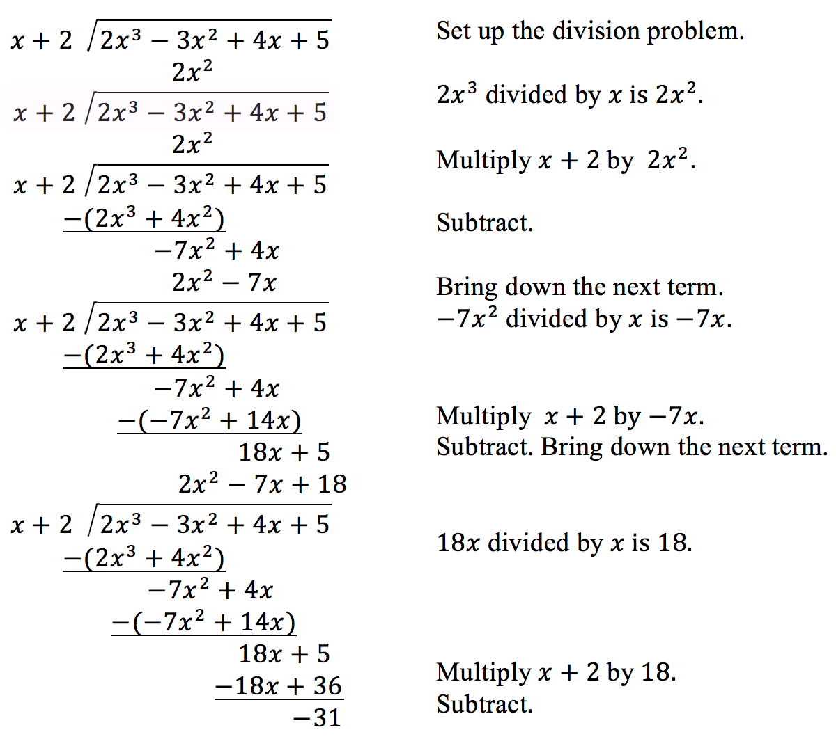
We have found
or
We can identify the dividend, the divisor, the quotient, and the remainder.
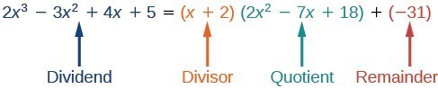
Writing the result in this manner illustrates the Division Algorithm.
The Division Algorithm states that, given a polynomial dividend [latex]f\left(x\right)\\[/latex] and a non-zero polynomial divisor [latex]d\left(x\right)\\[/latex] where the degree of [latex]d\left(x\right)\\[/latex] is less than or equal to the degree of [latex]f\left(x\right)\\[/latex], there exist unique polynomials [latex]q\left(x\right)\\[/latex] and [latex]r\left(x\right)\\[/latex] such that
[latex]q\left(x\right)\\[/latex] is the quotient and [latex]r\left(x\right)\\[/latex] is the remainder. The remainder is either equal to zero or has degree strictly less than [latex]d\left(x\right)\\[/latex].
If [latex]r\left(x\right)=0\\[/latex], then [latex]d\left(x\right)\\[/latex] divides evenly into [latex]f\left(x\right)\\[/latex]. This means that, in this case, both [latex]d\left(x\right)\\[/latex] and [latex]q\left(x\right)\\[/latex] are factors of [latex]f\left(x\right)\\[/latex].
Divide [latex]5{x}^{2}+3x - 2\\[/latex] by [latex]x+1\\[/latex].
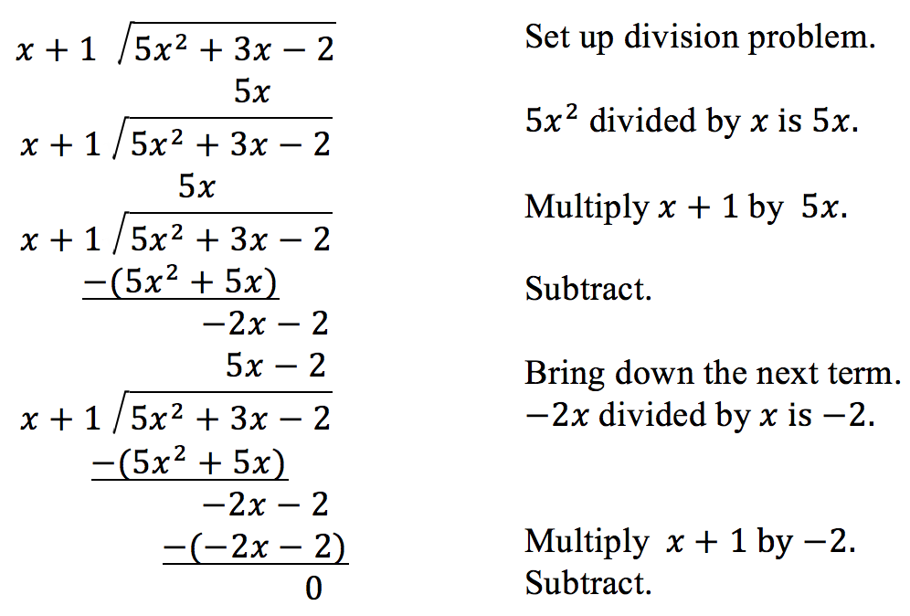
The quotient is [latex]5x - 2\\[/latex]. The remainder is 0. We write the result as
or
This division problem had a remainder of 0. This tells us that the dividend is divided evenly by the divisor, and that the divisor is a factor of the dividend.
Divide [latex]6{x}^{3}+11{x}^{2}-31x+15\\[/latex] by [latex]3x - 2\\[/latex].

There is a remainder of 1. We can express the result as:
We can check our work by using the Division Algorithm to rewrite the solution. Then multiply.
Notice, as we write our result,
As we’ve seen, long division of polynomials can involve many steps and be quite cumbersome. Synthetic division is a shorthand method of dividing polynomials for the special case of dividing by a linear factor whose leading coefficient is 1.
To illustrate the process, recall the example at the beginning of the section.
Divide [latex]2{x}^{3}-3{x}^{2}+4x+5\\[/latex] by [latex]x+2\\[/latex] using the long division algorithm.
The final form of the process looked like this:
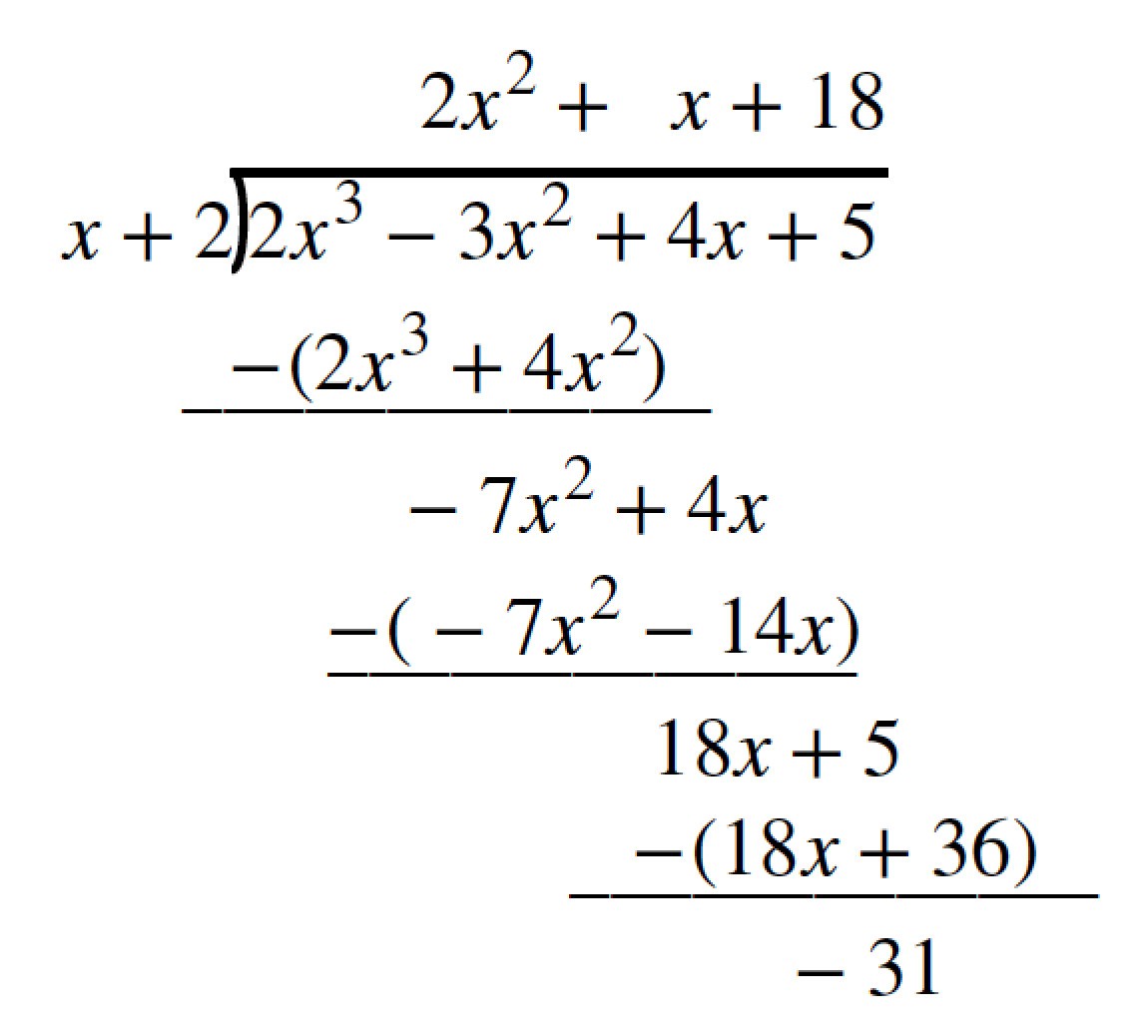
There is a lot of repetition in the table. If we don’t write the variables but, instead, line up their coefficients in columns under the division sign and also eliminate the partial products, we already have a simpler version of the entire problem.

Synthetic division carries this simplification even a few more steps. Collapse the table by moving each of the rows up to fill any vacant spots. Also, instead of dividing by 2, as we would in division of whole numbers, then multiplying and subtracting the middle product, we change the sign of the “divisor” to –2, multiply and add. The process starts by bringing down the leading coefficient.

We then multiply it by the “divisor” and add, repeating this process column by column, until there are no entries left. The bottom row represents the coefficients of the quotient; the last entry of the bottom row is the remainder. In this case, the quotient is [latex]2x{^2} -7x+18\\[/latex] and the remainder is –31. The process will be made more clear in Example 3.
Synthetic division is a shortcut that can be used when the divisor is a binomial in the form x – k. In synthetic division, only the coefficients are used in the division process.
Use synthetic division to divide [latex]5{x}^{2}-3x - 36\\[/latex] by [latex]x - 3\\[/latex].
Begin by setting up the synthetic division. Write k and the coefficients.

Bring down the lead coefficient. Multiply the lead coefficient by k.

Continue by adding the numbers in the second column. Multiply the resulting number by k. Write the result in the next column. Then add the numbers in the third column.

The result is [latex]5x+12\\[/latex]. The remainder is 0. So [latex]x - 3\\[/latex] is a factor of the original polynomial.
Just as with long division, we can check our work by multiplying the quotient by the divisor and adding the remainder.
[latex]\left(x - 3\right)\left(5x+12\right)+0=5{x}^{2}-3x - 36\\[/latex]
Use synthetic division to divide [latex]4{x}^{3}+10{x}^{2}-6x - 20\\[/latex] by [latex]x+2\\[/latex].
The binomial divisor is [latex]x+2\\[/latex] so [latex]k=-2\\[/latex]. Add each column, multiply the result by –2, and repeat until the last column is reached.

The result is [latex]4{x}^{2}+2x - 10\\[/latex]. The remainder is 0. Thus, [latex]x+2\\[/latex] is a factor of [latex]4{x}^{3}+10{x}^{2}-6x - 20\\[/latex].
The graph of the polynomial function [latex]f\left(x\right)=4{x}^{3}+10{x}^{2}-6x - 20\\[/latex] in Figure 2 shows a zero at [latex]x=k=-2\\[/latex]. This confirms that [latex]x+2\\[/latex] is a factor of [latex]4{x}^{3}+10{x}^{2}-6x - 20\\[/latex].
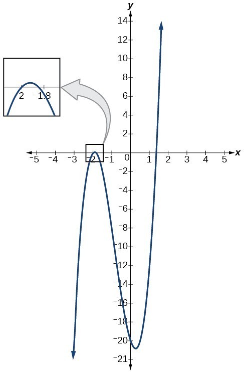
Figure 2
Use synthetic division to divide [latex]-9{x}^{4}+10{x}^{3}+7{x}^{2}-6\\[/latex] by [latex]x - 1\\[/latex].
Notice there is no x-term. We will use a zero as the coefficient for that term.
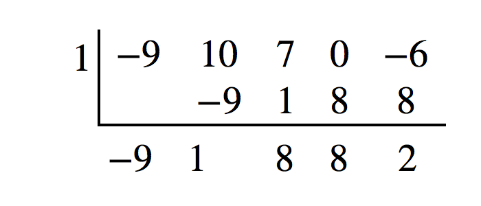
The result is [latex]-9{x}^{3}+{x}^{2}+8x+8+\frac{2}{x - 1}\\[/latex].
Use synthetic division to divide [latex]3{x}^{4}+18{x}^{3}-3x+40\\[/latex] by [latex]x+7\\[/latex].
Polynomial division can be used to solve a variety of application problems involving expressions for area and volume. We looked at an application at the beginning of this section. Now we will solve that problem in the following example.
The volume of a rectangular solid is given by the polynomial [latex]3{x}^{4}-3{x}^{3}-33{x}^{2}+54x\\[/latex]. The length of the solid is given by 3x and the width is given by x – 2. Find the height of the solid.
There are a few ways to approach this problem. We need to divide the expression for the volume of the solid by the expressions for the length and width. Let us create a sketch.
Figure 3
We can now write an equation by substituting the known values into the formula for the volume of a rectangular solid.
To solve for h, first divide both sides by 3x.
Now solve for h using synthetic division.

The quotient is [latex]{x}^{2}+x - 9\\[/latex] and the remainder is 0. The height of the solid is [latex]{x}^{2}+x - 9\\[/latex].
The area of a rectangle is given by [latex]3{x}^{3}+14{x}^{2}-23x+6\\[/latex]. The width of the rectangle is given by x + 6. Find an expression for the length of the rectangle.
| Division Algorithm | [latex]f\left(x\right)=d\left(x\right)q\left(x\right)+r\left(x\right)\\[/latex] where [latex]q\left(x\right)\ne 0\\[/latex] |
1. If division of a polynomial by a binomial results in a remainder of zero, what can be conclude?
2. If a polynomial of degree n is divided by a binomial of degree 1, what is the degree of the quotient?
For the following exercises, use long division to divide. Specify the quotient and the remainder.
3. [latex]\left({x}^{2}+5x - 1\right)\div \left(x - 1\right)\\[/latex]
4. [latex]\left(2{x}^{2}-9x - 5\right)\div \left(x - 5\right)\\[/latex]
5. [latex]\left(3{x}^{2}+23x+14\right)\div \left(x+7\right)\\[/latex]
6. [latex]\left(4{x}^{2}-10x+6\right)\div \left(4x+2\right)\\[/latex]
7. [latex]\left(6{x}^{2}-25x - 25\right)\div \left(6x+5\right)\\[/latex]
8. [latex]\left(-{x}^{2}-1\right)\div \left(x+1\right)\\[/latex]
9. [latex]\left(2{x}^{2}-3x+2\right)\div \left(x+2\right)\\[/latex]
10. [latex]\left({x}^{3}-126\right)\div \left(x - 5\right)\\[/latex]
11. [latex]\left(3{x}^{2}-5x+4\right)\div \left(3x+1\right)\\[/latex]
12. [latex]\left({x}^{3}-3{x}^{2}+5x - 6\right)\div \left(x - 2\right)\\[/latex]
13. [latex]\left(2{x}^{3}+3{x}^{2}-4x+15\right)\div \left(x+3\right)\\[/latex]
For the following exercises, use synthetic division to find the quotient.
14. [latex]\left(3{x}^{3}-2{x}^{2}+x - 4\right)\div \left(x+3\right)\\[/latex]
15. [latex]\left(2{x}^{3}-6{x}^{2}-7x+6\right)\div \left(x - 4\right)\\[/latex]
16. [latex]\left(6{x}^{3}-10{x}^{2}-7x - 15\right)\div \left(x+1\right)\\[/latex]
17. [latex]\left(4{x}^{3}-12{x}^{2}-5x - 1\right)\div \left(2x+1\right)\\[/latex]
18. [latex]\left(9{x}^{3}-9{x}^{2}+18x+5\right)\div \left(3x - 1\right)\\[/latex]
19. [latex]\left(3{x}^{3}-2{x}^{2}+x - 4\right)\div \left(x+3\right)\\[/latex]
20. [latex]\left(-6{x}^{3}+{x}^{2}-4\right)\div \left(2x - 3\right)\\[/latex]
21. [latex]\left(2{x}^{3}+7{x}^{2}-13x - 3\right)\div \left(2x - 3\right)\\[/latex]
22. [latex]\left(3{x}^{3}-5{x}^{2}+2x+3\right)\div \left(x+2\right)\\[/latex]
23. [latex]\left(4{x}^{3}-5{x}^{2}+13\right)\div \left(x+4\right)\\[/latex]
24. [latex]\left({x}^{3}-3x+2\right)\div \left(x+2\right)\\[/latex]
25. [latex]\left({x}^{3}-21{x}^{2}+147x - 343\right)\div \left(x - 7\right)\\[/latex]
26. [latex]\left({x}^{3}-15{x}^{2}+75x - 125\right)\div \left(x - 5\right)\\[/latex]
27. [latex]\left(9{x}^{3}-x+2\right)\div \left(3x - 1\right)\\[/latex]
28. [latex]\left(6{x}^{3}-{x}^{2}+5x+2\right)\div \left(3x+1\right)\\[/latex]
29. [latex]\left({x}^{4}+{x}^{3}-3{x}^{2}-2x+1\right)\div \left(x+1\right)\\[/latex]
30. [latex]\left({x}^{4}-3{x}^{2}+1\right)\div \left(x - 1\right)\\[/latex]
31. [latex]\left({x}^{4}+2{x}^{3}-3{x}^{2}+2x+6\right)\div \left(x+3\right)\\[/latex]
32. [latex]\left({x}^{4}-10{x}^{3}+37{x}^{2}-60x+36\right)\div \left(x - 2\right)\\[/latex]
33. [latex]\left({x}^{4}-8{x}^{3}+24{x}^{2}-32x+16\right)\div \left(x - 2\right)\\[/latex]
34. [latex]\left({x}^{4}+5{x}^{3}-3{x}^{2}-13x+10\right)\div \left(x+5\right)\\[/latex]
35. [latex]\left({x}^{4}-12{x}^{3}+54{x}^{2}-108x+81\right)\div \left(x - 3\right)\\[/latex]
36. [latex]\left(4{x}^{4}-2{x}^{3}-4x+2\right)\div \left(2x - 1\right)\\[/latex]
37. [latex]\left(4{x}^{4}+2{x}^{3}-4{x}^{2}+2x+2\right)\div \left(2x+1\right)\\[/latex]
For the following exercises, use the graph of the third-degree polynomial and one factor to write the factored form of the polynomial suggested by the graph. The leading coefficient is one.
38. Factor is [latex]{x}^{2}-x+3\\[/latex]

39. Factor is [latex]\left({x}^{2}+2x+4\right)\\[/latex]

40. Factor is [latex]{x}^{2}+2x+5\\[/latex]

41. Factor is [latex]{x}^{2}+x+1\\[/latex]

42. Factor is [latex]{x}^{2}+2x+2\\[/latex]

For the following exercises, use synthetic division to find the quotient and remainder.
43. [latex]\frac{4{x}^{3}-33}{x - 2}\\[/latex]
44. [latex]\frac{2{x}^{3}+25}{x+3}\\[/latex]
45. [latex]\frac{3{x}^{3}+2x - 5}{x - 1}\\[/latex]
46. [latex]\frac{-4{x}^{3}-{x}^{2}-12}{x+4}\\[/latex]
47. [latex]\frac{{x}^{4}-22}{x+2}\\[/latex]
For the following exercises, use a calculator with CAS to answer the questions.
48. Consider [latex]\frac{{x}^{k}-1}{x - 1}\\[/latex] with [latex]k=1, 2, 3\\[/latex]. What do you expect the result to be if k = 4?
49. Consider [latex]\frac{{x}^{k}+1}{x+1}\\[/latex] for [latex]k=1, 3, 5\\[/latex]. What do you expect the result to be if k = 7?
50. Consider [latex]\frac{{x}^{4}-{k}^{4}}{x-k}\\[/latex] for [latex]k=1, 2, 3\\[/latex]. What do you expect the result to be if k = 4?
51. Consider [latex]\frac{{x}^{k}}{x+1}\\[/latex] with [latex]k=1, 2, 3\\[/latex]. What do you expect the result to be if k = 4?
52. Consider [latex]\frac{{x}^{k}}{x - 1}\\[/latex] with [latex]k=1, 2, 3\\[/latex]. What do you expect the result to be if k = 4?
For the following exercises, use synthetic division to determine the quotient involving a complex number.
53. [latex]\frac{x+1}{x-i}\\[/latex]
54. [latex]\frac{{x}^{2}+1}{x-i}\\[/latex]
55. [latex]\frac{x+1}{x+i}\\[/latex]
56. [latex]\frac{{x}^{2}+1}{x+i}\\[/latex]
57. [latex]\frac{{x}^{3}+1}{x-i}\\[/latex]
For the following exercises, use the given length and area of a rectangle to express the width algebraically.
58. Length is [latex]x+5\\[/latex], area is [latex]2{x}^{2}+9x - 5\\[/latex].
59. Length is [latex]2x\text{ }+\text{ }5\\[/latex], area is [latex]4{x}^{3}+10{x}^{2}+6x+15\\[/latex]
60. Length is [latex]3x - 4\\[/latex], area is [latex]6{x}^{4}-8{x}^{3}+9{x}^{2}-9x - 4\\[/latex]
For the following exercises, use the given volume of a box and its length and width to express the height of the box algebraically.
61. Volume is [latex]12{x}^{3}+20{x}^{2}-21x - 36\\[/latex], length is [latex]2x+3\\[/latex], width is [latex]3x - 4\\[/latex].
62. Volume is [latex]18{x}^{3}-21{x}^{2}-40x+48\\[/latex], length is [latex]3x - 4\\[/latex], width is [latex]3x - 4\\[/latex].
63. Volume is [latex]10{x}^{3}+27{x}^{2}+2x - 24\\[/latex], length is [latex]5x - 4\\[/latex], width is [latex]2x+3\\[/latex].
64. Volume is [latex]10{x}^{3}+30{x}^{2}-8x - 24\\[/latex], length is 2, width is [latex]x+3\\[/latex].
For the following exercises, use the given volume and radius of a cylinder to express the height of the cylinder algebraically.
65. Volume is [latex]\pi \left(25{x}^{3}-65{x}^{2}-29x - 3\right)\\[/latex], radius is [latex]5x+1\\[/latex].
66. Volume is [latex]\pi \left(4{x}^{3}+12{x}^{2}-15x - 50\right)\\[/latex], radius is [latex]2x+5\\[/latex].
67. Volume is [latex]\pi \left(3{x}^{4}+24{x}^{3}+46{x}^{2}-16x - 32\right)\\[/latex], radius is [latex]x+4\\[/latex].
1. [latex]4{x}^{2}-8x+15-\frac{78}{4x+5}\\[/latex]
2. [latex]3{x}^{3}-3{x}^{2}+21x - 150+\frac{1,090}{x+7}\\[/latex]
3. [latex]3{x}^{2}-4x+1\\[/latex]
1. The binomial is a factor of the polynomial.
3. [latex]x+6+\frac{5}{x - 1}\text{,}\text{quotient:}x+6\text{,}\text{remainder:}\text{5}\\[/latex]
5. [latex]3x+2\text{,}\text{ quotient: }3x+2\text{, }\text{remainder: 0}\\[/latex]
7. [latex]x - 5\text{,}\text{quotient: }x - 5\text{,}\text{remainder: }\text{0}\\[/latex]
9. [latex]2x - 7+\frac{16}{x+2}\text{,}\text{quotient: }\text{ }2x - 7\text{,}\text{remainder: }\text{16}\\[/latex]
11. [latex]x - 2+\frac{6}{3x+1}\text{,}\text{quotient: }x - 2\text{,}\text{remainder: }\text{6}\\[/latex]
13. [latex]2{x}^{2}-3x+5\text{,}\text{quotient:}2{x}^{2}-3x+5\text{,}\text{remainder: }\text{0}\\[/latex]
15. [latex]2{x}^{2}+2x+1+\frac{10}{x - 4}\\[/latex]
17. [latex]2{x}^{2}-7x+1-\frac{2}{2x+1}\\[/latex]
19. [latex]3{x}^{2}-11x+34-\frac{106}{x+3}\\[/latex]
21. [latex]{x}^{2}+5x+1\\[/latex]
23. [latex]4{x}^{2}-21x+84-\frac{323}{x+4}\\[/latex]
25. [latex]{x}^{2}-14x+49\\[/latex]
27. [latex]3{x}^{2}+x+\frac{2}{3x - 1}\\[/latex]
29. [latex]{x}^{3}-3x+1\\[/latex]
31. [latex]{x}^{3}-{x}^{2}+2\\[/latex]
33. [latex]{x}^{3}-6{x}^{2}+12x - 8\\[/latex]
35. [latex]{x}^{3}-9{x}^{2}+27x - 27\\[/latex]
37. [latex]2{x}^{3}-2x+2\\[/latex]
39. [latex]\left(x - 1\right)\left({x}^{2}+2x+4\right)\\[/latex]
41. [latex]\left(x - 5\right)\left({x}^{2}+x+1\right)\\[/latex]
43. [latex]\text{Quotient: }4{x}^{2}+8x+16\text{,}\text{remainder: }-1\\[/latex]
45. [latex]\text{Quotient: }3{x}^{2}+3x+5\text{,}\text{remainder: }0\\[/latex]
47. [latex]\text{Quotient: }{x}^{3}-2{x}^{2}+4x - 8\text{,}\text{remainder: }-6\\[/latex]
49. [latex]{x}^{6}-{x}^{5}+{x}^{4}-{x}^{3}+{x}^{2}-x+1\\[/latex]
51. [latex]{x}^{3}-{x}^{2}+x - 1+\frac{1}{x+1}\\[/latex]
53. [latex]1+\frac{1+i}{x-i}\\[/latex]
55. [latex]1+\frac{1-i}{x+i}\\[/latex]
57. [latex]{x}^{2}-ix - 1+\frac{1-i}{x-i}\\[/latex]
59. [latex]2{x}^{2}+3\\[/latex]
61. [latex]2x+3\\[/latex]
63. [latex]x+2\\[/latex]
65. [latex]x - 3\\[/latex]
67. [latex]3{x}^{2}-2\\[/latex]
By the end of this lesson, you will be able to:
A new bakery offers decorated sheet cakes for children’s birthday parties and other special occasions. The bakery wants the volume of a small cake to be 351 cubic inches. The cake is in the shape of a rectangular solid. They want the length of the cake to be four inches longer than the width of the cake and the height of the cake to be one-third of the width. What should the dimensions of the cake pan be?
This problem can be solved by writing a cubic function and solving a cubic equation for the volume of the cake. In this section, we will discuss a variety of tools for writing polynomial functions and solving polynomial equations.
In the last section, we learned how to divide polynomials. We can now use polynomial division to evaluate polynomials using the Remainder Theorem. If the polynomial is divided by x – k, the remainder may be found quickly by evaluating the polynomial function at k, that is, f(k) Let’s walk through the proof of the theorem.
Recall that the Division Algorithm states that, given a polynomial dividend f(x) and a non-zero polynomial divisor d(x) where the degree of d(x) is less than or equal to the degree of f(x), there exist unique polynomials q(x) and r(x) such that
If the divisor, d(x), is x – k, this takes the form
Since the divisor x – k is linear, the remainder will be a constant, r. And, if we evaluate this for x = k, we have
In other words, f(k) is the remainder obtained by dividing f(x) by x – k.
If a polynomial [latex]f\left(x\right)\\[/latex] is divided by x – k, then the remainder is the value [latex]f\left(k\right)\\[/latex].
Use the Remainder Theorem to evaluate [latex]f\left(x\right)=6{x}^{4}-{x}^{3}-15{x}^{2}+2x - 7\\[/latex] at [latex]x=2\\[/latex].
To find the remainder using the Remainder Theorem, use synthetic division to divide the polynomial by [latex]x - 2\\[/latex].
The remainder is 25. Therefore, [latex]f\left(2\right)=25\\[/latex].
We can check our answer by evaluating [latex]f\left(2\right)\\[/latex].
Use the Remainder Theorem to evaluate [latex]f\left(x\right)=2{x}^{5}-3{x}^{4}-9{x}^{3}+8{x}^{2}+2\\[/latex]
at [latex]x=-3\\[/latex].
The Factor Theorem is another theorem that helps us analyze polynomial equations. It tells us how the zeros of a polynomial are related to the factors. Recall that the Division Algorithm tells us
If k is a zero, then the remainder r is [latex]f\left(k\right)=0\\[/latex] and [latex]f\left(x\right)=\left(x-k\right)q\left(x\right)+0\\[/latex] or [latex]f\left(x\right)=\left(x-k\right)q\left(x\right)\\[/latex].
Notice, written in this form, x – k is a factor of [latex]f\left(x\right)\\[/latex]. We can conclude if k is a zero of [latex]f\left(x\right)\\[/latex], then [latex]x-k\\[/latex] is a factor of [latex]f\left(x\right)\\[/latex].
Similarly, if [latex]x-k\\[/latex] is a factor of [latex]f\left(x\right)\\[/latex], then the remainder of the Division Algorithm [latex]f\left(x\right)=\left(x-k\right)q\left(x\right)+r\\[/latex] is 0. This tells us that k is a zero.
This pair of implications is the Factor Theorem. As we will soon see, a polynomial of degree n in the complex number system will have n zeros. We can use the Factor Theorem to completely factor a polynomial into the product of n factors. Once the polynomial has been completely factored, we can easily determine the zeros of the polynomial.
According to the Factor Theorem, k is a zero of [latex]f\left(x\right)\\[/latex] if and only if [latex]\left(x-k\right)\\[/latex] is a factor of [latex]f\left(x\right)\\[/latex].
Show that [latex]\left(x+2\right)\\[/latex] is a factor of [latex]{x}^{3}-6{x}^{2}-x+30\\[/latex]. Find the remaining factors. Use the factors to determine the zeros of the polynomial.
We can use synthetic division to show that [latex]\left(x+2\right)\\[/latex] is a factor of the polynomial.

The remainder is zero, so [latex]\left(x+2\right)\\[/latex] is a factor of the polynomial. We can use the Division Algorithm to write the polynomial as the product of the divisor and the quotient:
We can factor the quadratic factor to write the polynomial as
By the Factor Theorem, the zeros of [latex]{x}^{3}-6{x}^{2}-x+30\\[/latex] are –2, 3, and 5.
Use the Factor Theorem to find the zeros of [latex]f\left(x\right)={x}^{3}+4{x}^{2}-4x - 16\\[/latex] given that [latex]\left(x - 2\right)\\[/latex] is a factor of the polynomial.
Another use for the Remainder Theorem is to test whether a rational number is a zero for a given polynomial. But first we need a pool of rational numbers to test. The Rational Zero Theorem helps us to narrow down the number of possible rational zeros using the ratio of the factors of the constant term and factors of the leading coefficient of the polynomial
Consider a quadratic function with two zeros, [latex]x=\frac{2}{5}\\[/latex] and [latex]x=\frac{3}{4}\\[/latex].
By the Factor Theorem, these zeros have factors associated with them. Let us set each factor equal to 0, and then construct the original quadratic function absent its stretching factor.
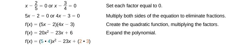
Notice that two of the factors of the constant term, 6, are the two numerators from the original rational roots: 2 and 3. Similarly, two of the factors from the leading coefficient, 20, are the two denominators from the original rational roots: 5 and 4.
We can infer that the numerators of the rational roots will always be factors of the constant term and the denominators will be factors of the leading coefficient. This is the essence of the Rational Zero Theorem; it is a means to give us a pool of possible rational zeros.
The Rational Zero Theorem states that, if the polynomial [latex]f\left(x\right)={a}_{n}{x}^{n}+{a}_{n - 1}{x}^{n - 1}+…+{a}_{1}x+{a}_{0}\\[/latex] has integer coefficients, then every rational zero of [latex]f\left(x\right)\\[/latex] has the form [latex]\frac{p}{q}\\[/latex] where p is a factor of the constant term [latex]{a}_{0}\\[/latex] and q is a factor of the leading coefficient [latex]{a}_{n}\\[/latex].
When the leading coefficient is 1, the possible rational zeros are the factors of the constant term.
List all possible rational zeros of [latex]f\left(x\right)=2{x}^{4}-5{x}^{3}+{x}^{2}-4\\[/latex].
The only possible rational zeros of [latex]f\left(x\right)\\[/latex] are the quotients of the factors of the last term, –4, and the factors of the leading coefficient, 2.
The constant term is –4; the factors of –4 are [latex]p=\pm 1,\pm 2,\pm 4\\[/latex].
The leading coefficient is 2; the factors of 2 are [latex]q=\pm 1,\pm 2\\[/latex].
If any of the four real zeros are rational zeros, then they will be of one of the following factors of –4 divided by one of the factors of 2.
Note that [latex]\frac{2}{2}=1\\[/latex] and [latex]\frac{4}{2}=2\\[/latex], which have already been listed. So we can shorten our list.
Use the Rational Zero Theorem to find the rational zeros of [latex]f\left(x\right)=2{x}^{3}+{x}^{2}-4x+1\\[/latex].
The Rational Zero Theorem tells us that if [latex]\frac{p}{q}\\[/latex] is a zero of [latex]f\left(x\right)\\[/latex], then p is a factor of 1 and q is a factor of 2.
The factors of 1 are [latex]\pm 1\\[/latex] and the factors of 2 are [latex]\pm 1\\[/latex] and [latex]\pm 2\\[/latex]. The possible values for [latex]\frac{p}{q}\\[/latex] are [latex]\pm 1\\[/latex] and [latex]\pm \frac{1}{2}\\[/latex]. These are the possible rational zeros for the function. We can determine which of the possible zeros are actual zeros by substituting these values for x in [latex]f\left(x\right)\\[/latex].
Of those, [latex]-1,-\frac{1}{2},\text{ and }\frac{1}{2}\\[/latex] are not zeros of [latex]f\left(x\right)\\[/latex]. 1 is the only rational zero of [latex]f\left(x\right)\\[/latex].
Use the Rational Zero Theorem to find the rational zeros of [latex]f\left(x\right)={x}^{3}-5{x}^{2}+2x+1\\[/latex].
The Rational Zero Theorem helps us to narrow down the list of possible rational zeros for a polynomial function. Once we have done this, we can use synthetic division repeatedly to determine all of the zeros of a polynomial function.
Find the zeros of [latex]f\left(x\right)=4{x}^{3}-3x - 1\\[/latex].
The Rational Zero Theorem tells us that if [latex]\frac{p}{q}\\[/latex] is a zero of [latex]f\left(x\right)\\[/latex], then p is a factor of –1 and q is a factor of 4.
The factors of –1 are [latex]\pm 1\\[/latex] and the factors of 4 are [latex]\pm 1,\pm 2\\[/latex], and [latex]\pm 4\\[/latex]. The possible values for [latex]\frac{p}{q}\\[/latex] are [latex]\pm 1,\pm \frac{1}{2}\\[/latex], and [latex]\pm \frac{1}{4}\\[/latex].
These are the possible rational zeros for the function. We will use synthetic division to evaluate each possible zero until we find one that gives a remainder of 0. Let’s begin with 1.

Dividing by [latex]\left(x - 1\right)\\[/latex] gives a remainder of 0, so 1 is a zero of the function. The polynomial can be written as
The quadratic is a perfect square. [latex]f\left(x\right)\\[/latex] can be written as
We already know that 1 is a zero. The other zero will have a multiplicity of 2 because the factor is squared. To find the other zero, we can set the factor equal to 0.
The zeros of the function are 1 and [latex]-\frac{1}{2}\\[/latex] with multiplicity 2.
Look at the graph of the function f in Figure 1. Notice, at [latex]x=-0.5\\[/latex], the graph bounces off the x-axis, indicating the even multiplicity (2,4,6…) for the zero –0.5. At [latex]x=1\\[/latex], the graph crosses the x-axis, indicating the odd multiplicity (1,3,5…) for the zero [latex]x=1\\[/latex].
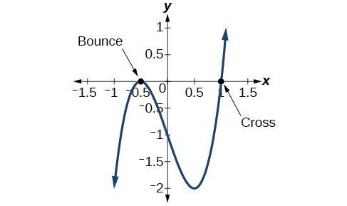
Figure 1
Now that we can find rational zeros for a polynomial function, we will look at a theorem that discusses the number of complex zeros of a polynomial function. The Fundamental Theorem of Algebra tells us that every polynomial function has at least one complex zero. This theorem forms the foundation for solving polynomial equations.
Suppose f is a polynomial function of degree four, and [latex]f\left(x\right)=0\\[/latex]. The Fundamental Theorem of Algebra states that there is at least one complex solution, call it [latex]{c}_{1}\\[/latex]. By the Factor Theorem, we can write [latex]f\left(x\right)\\[/latex] as a product of [latex]x-{c}_{\text{1}}\\[/latex] and a polynomial quotient. Since [latex]x-{c}_{\text{1}}\\[/latex] is linear, the polynomial quotient will be of degree three. Now we apply the Fundamental Theorem of Algebra to the third-degree polynomial quotient. It will have at least one complex zero, call it [latex]{c}_{\text{2}}\\[/latex]. So we can write the polynomial quotient as a product of [latex]x-{c}_{\text{2}}\\[/latex] and a new polynomial quotient of degree two. Continue to apply the Fundamental Theorem of Algebra until all of the zeros are found. There will be four of them and each one will yield a factor of [latex]f\left(x\right)\\[/latex].
We can use this theorem to argue that, if [latex]f\left(x\right)\\[/latex] is a polynomial of degree [latex]n>0\\[/latex], and a is a non-zero real number, then [latex]f\left(x\right)\\[/latex] has exactly n linear factors
where [latex]{c}_{1},{c}_{2},…,{c}_{n}\\[/latex] are complex numbers. Therefore, [latex]f\left(x\right)\\[/latex] has n roots if we allow for multiplicities.
Does every polynomial have at least one imaginary zero?
No. A complex number is not necessarily imaginary. Real numbers are also complex numbers.
Find the zeros of [latex]f\left(x\right)=3{x}^{3}+9{x}^{2}+x+3\\[/latex].
The Rational Zero Theorem tells us that if [latex]\frac{p}{q}\\[/latex] is a zero of [latex]f\left(x\right)\\[/latex], then p is a factor of 3 and q is a factor of 3.
The factors of 3 are [latex]\pm 1\\[/latex] and [latex]\pm 3\\[/latex]. The possible values for [latex]\frac{p}{q}\\[/latex], and therefore the possible rational zeros for the function, are [latex]\pm 3,\text{\pm 1, and }\pm \frac{1}{3}\\[/latex]. We will use synthetic division to evaluate each possible zero until we find one that gives a remainder of 0. Let’s begin with –3.
 Dividing by [latex]\left(x+3\right)\\[/latex] gives a remainder of 0, so –3 is a zero of the function. The polynomial can be written as
We can then set the quadratic equal to 0 and solve to find the other zeros of the function.
The zeros of [latex]f\left(x\right)\\[/latex] are –3 and [latex]\pm \frac{i\sqrt{3}}{3}\\[/latex].
Look at the graph of the function f. Notice that, at [latex]x=-3\\[/latex], the graph crosses the x-axis, indicating an odd multiplicity (1) for the zero [latex]x=-3\\[/latex]. Also note the presence of the two turning points. This means that, since there is a 3rd degree polynomial, we are looking at the maximum number of turning points. So, the end behavior of increasing without bound to the right and decreasing without bound to the left will continue. Thus, all the x-intercepts for the function are shown. So either the multiplicity of [latex]x=-3\\[/latex] is 1 and there are two complex solutions, which is what we found, or the multiplicity at [latex]x=-3\\[/latex] is three. Either way, our result is correct.

Figure 2
A vital implication of the Fundamental Theorem of Algebra, as we stated above, is that a polynomial function of degree n will have n zeros in the set of complex numbers, if we allow for multiplicities. This means that we can factor the polynomial function into n factors. The Linear Factorization Theorem tells us that a polynomial function will have the same number of factors as its degree, and that each factor will be in the form (x – c), where c is a complex number.
Let f be a polynomial function with real coefficients, and suppose [latex]a+bi\text{, }b\ne 0\\[/latex], is a zero of [latex]f\left(x\right)\\[/latex]. Then, by the Factor Theorem, [latex]x-\left(a+bi\right)\\[/latex] is a factor of [latex]f\left(x\right)\\[/latex]. For f to have real coefficients, [latex]x-\left(a-bi\right)\\[/latex] must also be a factor of [latex]f\left(x\right)\\[/latex]. This is true because any factor other than [latex]x-\left(a-bi\right)\\[/latex], when multiplied by [latex]x-\left(a+bi\right)\\[/latex], will leave imaginary components in the product. Only multiplication with conjugate pairs will eliminate the imaginary parts and result in real coefficients. In other words, if a polynomial function f with real coefficients has a complex zero [latex]a+bi\\[/latex], then the complex conjugate [latex]a-bi\\[/latex] must also be a zero of [latex]f\left(x\right)\\[/latex]. This is called the Complex Conjugate Theorem.
According to the Linear Factorization Theorem, a polynomial function will have the same number of factors as its degree, and each factor will be in the form [latex]\left(x-c\right)\\[/latex], where c is a complex number.
If the polynomial function f has real coefficients and a complex zero in the form [latex]a+bi\\[/latex], then the complex conjugate of the zero, [latex]a-bi\\[/latex], is also a zero.
Find a fourth degree polynomial with real coefficients that has zeros of –3, 2, i, such that [latex]f\left(-2\right)=100\\[/latex].
Because [latex]x=i\\[/latex] is a zero, by the Complex Conjugate Theorem [latex]x=-i\\[/latex] is also a zero. The polynomial must have factors of [latex]\left(x+3\right),\left(x - 2\right),\left(x-i\right)\\[/latex], and [latex]\left(x+i\right)\\[/latex]. Since we are looking for a degree 4 polynomial, and now have four zeros, we have all four factors. Let’s begin by multiplying these factors.
We need to find a to ensure [latex]f\left(-2\right)=100\\[/latex]. Substitute [latex]x=-2\\[/latex] and [latex]f\left(2\right)=100\\[/latex]
into [latex]f\left(x\right)\\[/latex].
So the polynomial function is
or
We found that both i and –i were zeros, but only one of these zeros needed to be given. If i is a zero of a polynomial with real coefficients, then –i must also be a zero of the polynomial because –i is the complex conjugate of i.
If 2 + 3i were given as a zero of a polynomial with real coefficients, would 2 – 3i also need to be a zero?
Yes. When any complex number with an imaginary component is given as a zero of a polynomial with real coefficients, the conjugate must also be a zero of the polynomial.
Find a third degree polynomial with real coefficients that has zeros of 5 and –2i such that [latex]f\left(1\right)=10\\[/latex].
There is a straightforward way to determine the possible numbers of positive and negative real zeros for any polynomial function. If the polynomial is written in descending order, Descartes’ Rule of Signs tells us of a relationship between the number of sign changes in [latex]f\left(x\right)\\[/latex] and the number of positive real zeros. For example, the polynomial function below has one sign change.
This tells us that the function must have 1 positive real zero.
There is a similar relationship between the number of sign changes in [latex]f\left(-x\right)\\[/latex] and the number of negative real zeros.
In this case, [latex]f\left(\mathrm{-x}\right)\\[/latex] has 3 sign changes. This tells us that [latex]f\left(x\right)\\[/latex] could have 3 or 1 negative real zeros.
According to Descartes’ Rule of Signs, if we let [latex]f\left(x\right)={a}_{n}{x}^{n}+{a}_{n - 1}{x}^{n - 1}+…+{a}_{1}x+{a}_{0}\\[/latex] be a polynomial function with real coefficients:
Use Descartes’ Rule of Signs to determine the possible numbers of positive and negative real zeros for [latex]f\left(x\right)=-{x}^{4}-3{x}^{3}+6{x}^{2}-4x - 12\\[/latex].
Begin by determining the number of sign changes.

There are two sign changes, so there are either 2 or 0 positive real roots. Next, we examine [latex]f\left(-x\right)\\[/latex] to determine the number of negative real roots.
[latex]\begin{cases}f\left(-x\right)=-{\left(-x\right)}^{4}-3{\left(-x\right)}^{3}+6{\left(-x\right)}^{2}-4\left(-x\right)-12\hfill \\ f\left(-x\right)=-{x}^{4}+3{x}^{3}+6{x}^{2}+4x - 12\hfill \end{cases}\\[/latex]
Again, there are two sign changes, so there are either 2 or 0 negative real roots.
There are four possibilities, as we can see below.
| Positive Real Zeros | Negative Real Zeros | Complex Zeros | Total Zeros |
|---|---|---|---|
| 2 | 2 | 0 | 4 |
| 2 | 0 | 2 | 4 |
| 0 | 2 | 2 | 4 |
| 0 | 0 | 4 | 4 |
We can confirm the numbers of positive and negative real roots by examining a graph of the function. We can see from the graph in Figure 3 that the function has 0 positive real roots and 2 negative real roots.
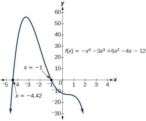
Figure 3
Use Descartes’ Rule of Signs to determine the maximum possible numbers of positive and negative real zeros for [latex]f\left(x\right)=2{x}^{4}-10{x}^{3}+11{x}^{2}-15x+12\\[/latex]. Use a graph to verify the numbers of positive and negative real zeros for the function.
We have now introduced a variety of tools for solving polynomial equations. Let’s use these tools to solve the bakery problem from the beginning of the section.
A new bakery offers decorated sheet cakes for children’s birthday parties and other special occasions. The bakery wants the volume of a small cake to be 351 cubic inches. The cake is in the shape of a rectangular solid. They want the length of the cake to be four inches longer than the width of the cake and the height of the cake to be one-third of the width. What should the dimensions of the cake pan be?
Begin by writing an equation for the volume of the cake. The volume of a rectangular solid is given by [latex]V=lwh\\[/latex]. We were given that the length must be four inches longer than the width, so we can express the length of the cake as [latex]l=w+4\\[/latex]. We were given that the height of the cake is one-third of the width, so we can express the height of the cake as [latex]h=\frac{1}{3}w\\[/latex]. Let’s write the volume of the cake in terms of width of the cake.
Substitute the given volume into this equation.
Descartes’ rule of signs tells us there is one positive solution. The Rational Zero Theorem tells us that the possible rational zeros are [latex]\pm 3,\pm 9,\pm 13,\pm 27,\pm 39,\pm 81,\pm 117,\pm 351\\[/latex], and [latex]\pm 1053\\[/latex]. We can use synthetic division to test these possible zeros. Only positive numbers make sense as dimensions for a cake, so we need not test any negative values. Let’s begin by testing values that make the most sense as dimensions for a small sheet cake. Use synthetic division to check [latex]x=1\\[/latex].

Since 1 is not a solution, we will check [latex]x=3\\[/latex].
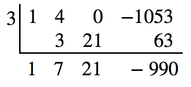
Since 3 is not a solution either, we will test [latex]x=9\\[/latex].
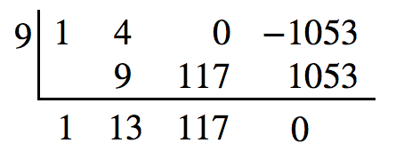
Synthetic division gives a remainder of 0, so 9 is a solution to the equation. We can use the relationships between the width and the other dimensions to determine the length and height of the sheet cake pan.
The sheet cake pan should have dimensions 13 inches by 9 inches by 3 inches.
A shipping container in the shape of a rectangular solid must have a volume of 84 cubic meters. The client tells the manufacturer that, because of the contents, the length of the container must be one meter longer than the width, and the height must be one meter greater than twice the width. What should the dimensions of the container be?
1. Describe a use for the Remainder Theorem.
2. Explain why the Rational Zero Theorem does not guarantee finding zeros of a polynomial function.
3. What is the difference between rational and real zeros?
4. If Descartes’ Rule of Signs reveals a no change of signs or one sign of changes, what specific conclusion can be drawn?
5. If synthetic division reveals a zero, why should we try that value again as a possible solution?
For the following exercises, use the Remainder Theorem to find the remainder.
6. [latex]\left({x}^{4}-9{x}^{2}+14\right)\div \left(x - 2\right)\\[/latex]
7. [latex]\left(3{x}^{3}-2{x}^{2}+x - 4\right)\div \left(x+3\right)\\[/latex]
8. [latex]\left({x}^{4}+5{x}^{3}-4x - 17\right)\div \left(x+1\right)\\[/latex]
9. [latex]\left(-3{x}^{2}+6x+24\right)\div \left(x - 4\right)\\[/latex]
10. [latex]\left(5{x}^{5}-4{x}^{4}+3{x}^{3}-2{x}^{2}+x - 1\right)\div \left(x+6\right)\\[/latex]
11. [latex]\left({x}^{4}-1\right)\div \left(x - 4\right)\\[/latex]
12. [latex]\left(3{x}^{3}+4{x}^{2}-8x+2\right)\div \left(x - 3\right)\\[/latex]
13. [latex]\left(4{x}^{3}+5{x}^{2}-2x+7\right)\div \left(x+2\right)\\[/latex]
For the following exercises, use the Factor Theorem to find all real zeros for the given polynomial function and one factor.
14. [latex]f\left(x\right)=2{x}^{3}-9{x}^{2}+13x - 6;\text{ }x - 1\\[/latex]
15. [latex]f\left(x\right)=2{x}^{3}+{x}^{2}-5x+2;\text{ }x+2\\[/latex]
16. [latex]f\left(x\right)=3{x}^{3}+{x}^{2}-20x+12;\text{ }x+3\\[/latex]
17. [latex]f\left(x\right)=2{x}^{3}+3{x}^{2}+x+6;x+2\\[/latex]
18. [latex]f\left(x\right)=-5{x}^{3}+16{x}^{2}-9;x - 3\\[/latex]
19. [latex]{x}^{3}+3{x}^{2}+4x+12;x+3\\[/latex]
20. [latex]4{x}^{3}-7x+3;x - 1\\[/latex]
21. [latex]2{x}^{3}+5{x}^{2}-12x - 30,\text{ }2x+5\\[/latex]
For the following exercises, use the Rational Zero Theorem to find all real zeros.
22. [latex]{x}^{3}-3{x}^{2}-10x+24=0\\[/latex]
23. [latex]2{x}^{3}+7{x}^{2}-10x - 24=0\\[/latex]
24. [latex]{x}^{3}+2{x}^{2}-9x - 18=0\\[/latex]
25. [latex]{x}^{3}+5{x}^{2}-16x - 80=0\\[/latex]
26. [latex]{x}^{3}-3{x}^{2}-25x+75=0\\[/latex]
27. [latex]2{x}^{3}-3{x}^{2}-32x - 15=0\\[/latex]
28. [latex]2{x}^{3}+{x}^{2}-7x - 6=0\\[/latex]
29. [latex]2{x}^{3}-3{x}^{2}-x+1=0\\[/latex]
30. [latex]3{x}^{3}-{x}^{2}-11x - 6=0\\[/latex]
31. [latex]2{x}^{3}-5{x}^{2}+9x - 9=0\\[/latex]
32. [latex]2{x}^{3}-3{x}^{2}+4x+3=0\\[/latex]
33. [latex]{x}^{4}-2{x}^{3}-7{x}^{2}+8x+12=0\\[/latex]
34. [latex]{x}^{4}+2{x}^{3}-9{x}^{2}-2x+8=0\\[/latex]
35. [latex]4{x}^{4}+4{x}^{3}-25{x}^{2}-x+6=0\\[/latex]
36. [latex]2{x}^{4}-3{x}^{3}-15{x}^{2}+32x - 12=0\\[/latex]
37. [latex]{x}^{4}+2{x}^{3}-4{x}^{2}-10x - 5=0\\[/latex]
38. [latex]4{x}^{3}-3x+1=0\\[/latex]
39. [latex]8{x}^{{}^{4}}+26{x}^{3}+39{x}^{2}+26x+6\\[/latex]
For the following exercises, find all complex solutions (real and non-real).
40. [latex]{x}^{3}+{x}^{2}+x+1=0\\[/latex]
41. [latex]{x}^{3}-8{x}^{2}+25x - 26=0\\[/latex]
42. [latex]{x}^{3}+13{x}^{2}+57x+85=0\\[/latex]
43. [latex]3{x}^{3}-4{x}^{2}+11x+10=0\\[/latex]
44. [latex]{x}^{4}+2{x}^{3}+22{x}^{2}+50x - 75=0\\[/latex]
45. [latex]2{x}^{3}-3{x}^{2}+32x+17=0\\[/latex]
For the following exercises, use Descartes’ Rule to determine the possible number of positive and negative solutions. Confirm with the given graph.
46. [latex]f\left(x\right)={x}^{3}-1\\[/latex]
47. [latex]f\left(x\right)={x}^{4}-{x}^{2}-1\\[/latex]
48. [latex]f\left(x\right)={x}^{3}-2{x}^{2}-5x+6\\[/latex]
49. [latex]f\left(x\right)={x}^{3}-2{x}^{2}+x - 1\\[/latex]
50. [latex]f\left(x\right)={x}^{4}+2{x}^{3}-12{x}^{2}+14x - 5\\[/latex]
51. [latex]f\left(x\right)=2{x}^{3}+37{x}^{2}+200x+300\\[/latex]
52. [latex]f\left(x\right)={x}^{3}-2{x}^{2}-16x+32\\[/latex]
53. [latex]f\left(x\right)=2{x}^{4}-5{x}^{3}-5{x}^{2}+5x+3\\[/latex]
54. [latex]f\left(x\right)=2{x}^{4}-5{x}^{3}-14{x}^{2}+20x+8\\[/latex]
55. [latex]f\left(x\right)=10{x}^{4}-21{x}^{2}+11\\[/latex]
For the following exercises, list all possible rational zeros for the functions.
56. [latex]f\left(x\right)={x}^{4}+3{x}^{3}-4x+4\\[/latex]
57. [latex]f\left(x\right)=2{x}^{{}^{3}}+3{x}^{2}-8x+5\\[/latex]
58. [latex]f\left(x\right)=3{x}^{{}^{3}}+5{x}^{2}-5x+4\\[/latex]
59. [latex]f\left(x\right)=6{x}^{4}-10{x}^{2}+13x+1\\[/latex]
60. [latex]f\left(x\right)=4{x}^{5}-10{x}^{4}+8{x}^{3}+{x}^{2}-8\\[/latex]
For the following exercises, use your calculator to graph the polynomial function. Based on the graph, find the rational zeros. All real solutions are rational.
61. [latex]f\left(x\right)=6{x}^{3}-7{x}^{2}+1\\[/latex]
62. [latex]f\left(x\right)=4{x}^{3}-4{x}^{2}-13x - 5\\[/latex]
63. [latex]f\left(x\right)=8{x}^{3}-6{x}^{2}-23x+6\\[/latex]
64. [latex]f\left(x\right)=12{x}^{4}+55{x}^{3}+12{x}^{2}-117x+54\\[/latex]
65. [latex]f\left(x\right)=16{x}^{4}-24{x}^{3}+{x}^{2}-15x+25\\[/latex]
For the following exercises, construct a polynomial function of least degree possible using the given information.
66. Real roots: –1, 1, 3 and [latex]\left(2,f\left(2\right)\right)=\left(2,4\right)\\[/latex]
67. Real roots: –1 (with multiplicity 2 and 1) and [latex]\left(2,f\left(2\right)\right)=\left(2,4\right)\\[/latex]
68. Real roots: –2, [latex]\frac{1}{2}\\[/latex] (with multiplicity 2) and [latex]\left(-3,f\left(-3\right)\right)=\left(-3,5\right)\\[/latex]
69. Real roots: [latex]-\frac{1}{2}\\[/latex], 0, [latex]\frac{1}{2}\\[/latex] and [latex]\left(-2,f\left(-2\right)\right)=\left(-2,6\right)\\[/latex]
70. Real roots: –4, –1, 1, 4 and [latex]\left(-2,f\left(-2\right)\right)=\left(-2,10\right)\\[/latex]
For the following exercises, find the dimensions of the box described.
71. The length is twice as long as the width. The height is 2 inches greater than the width. The volume is 192 cubic inches.
72. The length, width, and height are consecutive whole numbers. The volume is 120 cubic inches.
73. The length is one inch more than the width, which is one inch more than the height. The volume is 86.625 cubic inches.
74. The length is three times the height and the height is one inch less than the width. The volume is 108 cubic inches.
75. The length is 3 inches more than the width. The width is 2 inches more than the height. The volume is 120 cubic inches.
For the following exercises, find the dimensions of the right circular cylinder described.
76. The radius is 3 inches more than the height. The volume is [latex]16\pi \\[/latex] cubic meters.
77. The height is one less than one half the radius. The volume is [latex]72\pi \\[/latex] cubic meters.
78. The radius and height differ by one meter. The radius is larger and the volume is [latex]48\pi \\[/latex] cubic meters.
79. The radius and height differ by two meters. The height is greater and the volume is [latex]28.125\pi \\[/latex]
cubic meters.
80. The radius is [latex]\frac{1}{3}\\[/latex] meter greater than the height. The volume is [latex]\frac{98}{9}\pi \\[/latex]
cubic meters.
1. [latex]f\left(-3\right)=-412\\[/latex]
2. The zeros are 2, –2, and –4.
3. There are no rational zeros.
4. The zeros are [latex]\text{-4, }\frac{1}{2},\text{ and 1}\text{.}\\[/latex]
5. [latex]f\left(x\right)=-\frac{1}{2}{x}^{3}+\frac{5}{2}{x}^{2}-2x+10\\[/latex]
6. There must be 4, 2, or 0 positive real roots and 0 negative real roots. The graph shows that there are 2 positive real zeros and 0 negative real zeros.
7. 3 meters by 4 meters by 7 meters
1. The theorem can be used to evaluate a polynomial.
3. Rational zeros can be expressed as fractions whereas real zeros include irrational numbers.
5. Polynomial functions can have repeated zeros, so the fact that number is a zero doesn’t preclude it being a zero again.
7. –106
9. 0
11. 255
13. –1
15. –2, 1, [latex]\frac{1}{2}\\[/latex]
17. –2
19. –3
21. [latex]-\frac{5}{2}, \sqrt{6}, -\sqrt{6}\\[/latex]
23. [latex]2, -4, -\frac{3}{2}\\[/latex]
25. 4, –4, –5
27. [latex]5, -3, -\frac{1}{2}\\[/latex]
29. [latex]\frac{1}{2}, \frac{1+\sqrt{5}}{2}, \frac{1-\sqrt{5}}{2}\\[/latex]
31. [latex]\frac{3}{2}\\[/latex]
33. 2, 3, –1, –2
35. [latex]\frac{1}{2}, -\frac{1}{2}, 2, -3\\[/latex]
37. [latex]-1, -1, \sqrt{5}, -\sqrt{5}\\[/latex]
39. [latex]-\frac{3}{4}, -\frac{1}{2}\\[/latex]
41. [latex]2, 3+2i, 3 - 2i\\[/latex]
43. [latex]-\frac{2}{3}, 1+2i, 1 - 2i\\[/latex]
45. [latex]-\frac{1}{2}, 1+4i, 1 - 4i\\[/latex]
47. 1 positive, 1 negative

49. 3 or 1 positive, 0 negative

51. 0 positive, 3 or 1 negative

53. 2 or 0 positive, 2 or 0 negative

55. 2 or 0 positive, 2 or 0 negative

57. [latex]\pm 5, \pm 1, \pm \frac{5}{2}\\[/latex]
59. [latex]\pm 1, \pm \frac{1}{2}, \pm \frac{1}{3}, \pm \frac{1}{6}\\[/latex]
61. [latex]1, \frac{1}{2}, -\frac{1}{3}\\[/latex]
63. [latex]2, \frac{1}{4}, -\frac{3}{2}\\[/latex]
65. [latex]\frac{5}{4}\\[/latex]
67. [latex]f\left(x\right)=\frac{4}{9}\left({x}^{3}+{x}^{2}-x - 1\right)\\[/latex]
69. [latex]f\left(x\right)=-\frac{1}{5}\left(4{x}^{3}-x\right)\\[/latex]
71. 8 by 4 by 6 inches
73. 5.5 by 4.5 by 3.5 inches
75. 8 by 5 by 3 inches
77. Radius = 6 meters, Height = 2 meters
79. Radius = 2.5 meters, Height = 4.5 meters
By the end of this lesson, you will be able to:
Suppose we know that the cost of making a product is dependent on the number of items, x, produced. This is given by the equation [latex]C\left(x\right)=15,000x - 0.1{x}^{2}+1000\\[/latex]. If we want to know the average cost for producing x items, we would divide the cost function by the number of items, x.
The average cost function, which yields the average cost per item for x items produced, is
Many other application problems require finding an average value in a similar way, giving us variables in the denominator. Written without a variable in the denominator, this function will contain a negative integer power.
In the last few sections, we have worked with polynomial functions, which are functions with non-negative integers for exponents. In this section, we explore rational functions, which have variables in the denominator.
We have seen the graphs of the basic reciprocal function and the squared reciprocal function from our study of toolkit functions. Examine these graphs and notice some of their features.
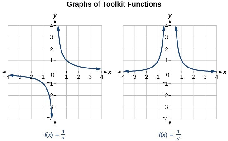
Figure 1
Several things are apparent if we examine the graph of [latex]f\left(x\right)=\frac{1}{x}\\[/latex].
To summarize, we use arrow notation to show that x or [latex]f\left(x\right)\\[/latex] is approaching a particular value.
| Arrow Notation | |
|---|---|
| Symbol | Meaning |
| [latex]x\to {a}^{-}\\[/latex] | x approaches a from the left (x < a but close to a) |
| [latex]x\to {a}^{+}\\[/latex] | x approaches a from the right (x > a but close to a) |
| [latex]x\to \infty\\ [/latex] | x approaches infinity (x increases without bound) |
| [latex]x\to -\infty \\[/latex] | x approaches negative infinity (x decreases without bound) |
| [latex]f\left(x\right)\to \infty \\[/latex] | the output approaches infinity (the output increases without bound) |
| [latex]f\left(x\right)\to -\infty \\[/latex] | the output approaches negative infinity (the output decreases without bound) |
| [latex]f\left(x\right)\to a\\[/latex] | the output approaches a |
Let’s begin by looking at the reciprocal function, [latex]f\left(x\right)=\frac{1}{x}\\[/latex]. We cannot divide by zero, which means the function is undefined at [latex]x=0\\[/latex]; so zero is not in the domain. As the input values approach zero from the left side (becoming very small, negative values), the function values decrease without bound (in other words, they approach negative infinity). We can see this behavior in the table below.
| x | –0.1 | –0.01 | –0.001 | –0.0001 |
| [latex]f\left(x\right)=\frac{1}{x}\\[/latex] | –10 | –100 | –1000 | –10,000 |
We write in arrow notation
As the input values approach zero from the right side (becoming very small, positive values), the function values increase without bound (approaching infinity). We can see this behavior in the table below.
| x | 0.1 | 0.01 | 0.001 | 0.0001 |
| [latex]f\left(x\right)=\frac{1}{x}\\[/latex] | 10 | 100 | 1000 | 10,000 |
We write in arrow notation
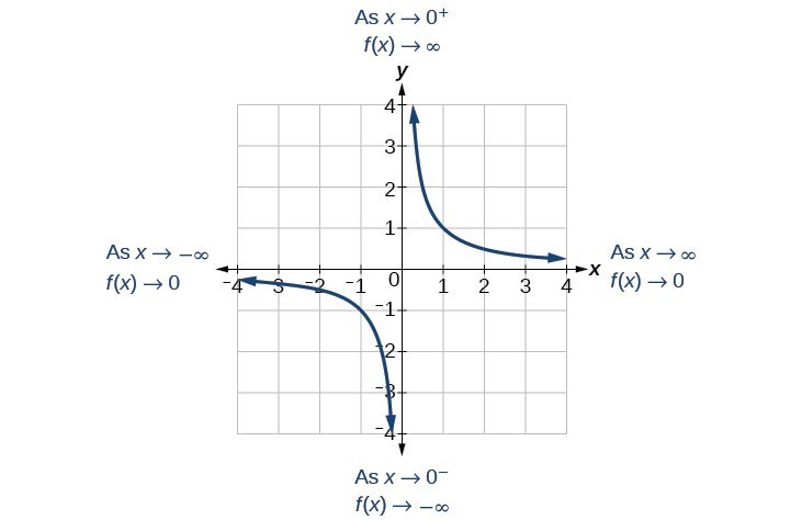
Figure 2
This behavior creates a vertical asymptote, which is a vertical line that the graph approaches but never crosses. In this case, the graph is approaching the vertical line x = 0 as the input becomes close to zero.
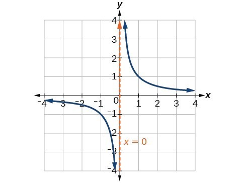
Figure 3
A vertical asymptote of a graph is a vertical line [latex]x=a\\[/latex] where the graph tends toward positive or negative infinity as the inputs approach a. We write
As the values of x approach infinity, the function values approach 0. As the values of x approach negative infinity, the function values approach 0. Symbolically, using arrow notation
[latex]\text{As }x\to \infty ,f\left(x\right)\to 0,\text{and as }x\to -\infty ,f\left(x\right)\to 0\\[/latex].
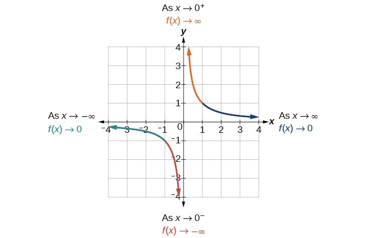
Figure 4
Based on this overall behavior and the graph, we can see that the function approaches 0 but never actually reaches 0; it seems to level off as the inputs become large. This behavior creates a horizontal asymptote, a horizontal line that the graph approaches as the input increases or decreases without bound. In this case, the graph is approaching the horizontal line [latex]y=0\\[/latex].
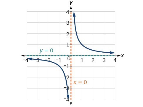
Figure 5
A horizontal asymptote of a graph is a horizontal line [latex]y=b\\[/latex] where the graph approaches the line as the inputs increase or decrease without bound. We write
Use arrow notation to describe the end behavior and local behavior of the function graphed in Figure 6.
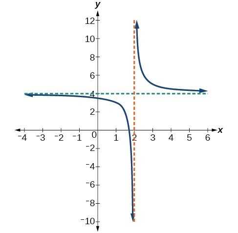
Figure 6
Notice that the graph is showing a vertical asymptote at [latex]x=2\\[/latex], which tells us that the function is undefined at [latex]x=2\\[/latex].
And as the inputs decrease without bound, the graph appears to be leveling off at output values of 4, indicating a horizontal asymptote at [latex]y=4\\[/latex]. As the inputs increase without bound, the graph levels off at 4.
Use arrow notation to describe the end behavior and local behavior for the reciprocal squared function.
Sketch a graph of the reciprocal function shifted two units to the left and up three units. Identify the horizontal and vertical asymptotes of the graph, if any.
Shifting the graph left 2 and up 3 would result in the function
or equivalently, by giving the terms a common denominator,
The graph of the shifted function is displayed in Figure 7.
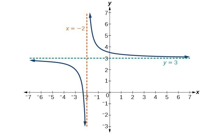
Figure 7
Notice that this function is undefined at [latex]x=-2\\[/latex], and the graph also is showing a vertical asymptote at [latex]x=-2\\[/latex].
As the inputs increase and decrease without bound, the graph appears to be leveling off at output values of 3, indicating a horizontal asymptote at [latex]y=3\\[/latex].
Notice that horizontal and vertical asymptotes are shifted left 2 and up 3 along with the function.
Sketch the graph, and find the horizontal and vertical asymptotes of the reciprocal squared function that has been shifted right 3 units and down 4 units.
In Example 2, we shifted a toolkit function in a way that resulted in the function [latex]f\left(x\right)=\frac{3x+7}{x+2}\\[/latex]. This is an example of a rational function. A rational function is a function that can be written as the quotient of two polynomial functions. Many real-world problems require us to find the ratio of two polynomial functions. Problems involving rates and concentrations often involve rational functions.
A rational function is a function that can be written as the quotient of two polynomial functions [latex]P\left(x\right) \text{and} Q\left(x\right)\\[/latex].
A large mixing tank currently contains 100 gallons of water into which 5 pounds of sugar have been mixed. A tap will open pouring 10 gallons per minute of water into the tank at the same time sugar is poured into the tank at a rate of 1 pound per minute. Find the concentration (pounds per gallon) of sugar in the tank after 12 minutes. Is that a greater concentration than at the beginning?
Let t be the number of minutes since the tap opened. Since the water increases at 10 gallons per minute, and the sugar increases at 1 pound per minute, these are constant rates of change. This tells us the amount of water in the tank is changing linearly, as is the amount of sugar in the tank. We can write an equation independently for each:
The concentration, C, will be the ratio of pounds of sugar to gallons of water
The concentration after 12 minutes is given by evaluating [latex]C\left(t\right)\\[/latex] at [latex]t=\text{ }12\\[/latex].
This means the concentration is 17 pounds of sugar to 220 gallons of water.
At the beginning, the concentration is
Since [latex]\frac{17}{220}\approx 0.08>\frac{1}{20}=0.05\\[/latex], the concentration is greater after 12 minutes than at the beginning.
To find the horizontal asymptote, divide the leading coefficient in the numerator by the leading coefficient in the denominator:
Notice the horizontal asymptote is [latex]y=\text{ }0.1\\[/latex]. This means the concentration, C, the ratio of pounds of sugar to gallons of water, will approach 0.1 in the long term.
There are 1,200 freshmen and 1,500 sophomores at a prep rally at noon. After 12 p.m., 20 freshmen arrive at the rally every five minutes while 15 sophomores leave the rally. Find the ratio of freshmen to sophomores at 1 p.m.
A vertical asymptote represents a value at which a rational function is undefined, so that value is not in the domain of the function. A reciprocal function cannot have values in its domain that cause the denominator to equal zero. In general, to find the domain of a rational function, we need to determine which inputs would cause division by zero.
The domain of a rational function includes all real numbers except those that cause the denominator to equal zero.
Find the domain of [latex]f\left(x\right)=\frac{x+3}{{x}^{2}-9}\\[/latex].
Begin by setting the denominator equal to zero and solving.
The denominator is equal to zero when [latex]x=\pm 3\\[/latex]. The domain of the function is all real numbers except [latex]x=\pm 3\\[/latex].
A graph of this function confirms that the function is not defined when [latex]x=\pm 3\\[/latex].
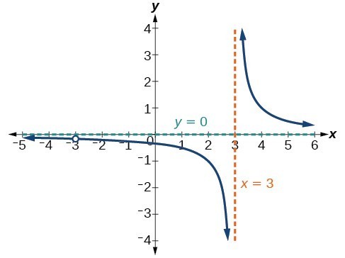
Figure 8
There is a vertical asymptote at [latex]x=3\\[/latex] and a hole in the graph at [latex]x=-3\\[/latex]. We will discuss these types of holes in greater detail later in this section.
Find the domain of [latex]f\left(x\right)=\frac{4x}{5\left(x - 1\right)\left(x - 5\right)}\\[/latex].
By looking at the graph of a rational function, we can investigate its local behavior and easily see whether there are asymptotes. We may even be able to approximate their location. Even without the graph, however, we can still determine whether a given rational function has any asymptotes, and calculate their location.
The vertical asymptotes of a rational function may be found by examining the factors of the denominator that are not common to the factors in the numerator. Vertical asymptotes occur at the zeros of such factors.
Find the vertical asymptotes of the graph of [latex]k\left(x\right)=\frac{5+2{x}^{2}}{2-x-{x}^{2}}\\[/latex].
First, factor the numerator and denominator.
To find the vertical asymptotes, we determine where this function will be undefined by setting the denominator equal to zero:
Neither [latex]x=-2\\[/latex] nor [latex]x=1\\[/latex] are zeros of the numerator, so the two values indicate two vertical asymptotes. Figure 9 confirms the location of the two vertical asymptotes.
Figure 9
Occasionally, a graph will contain a hole: a single point where the graph is not defined, indicated by an open circle. We call such a hole a removable discontinuity.
For example, the function [latex]f\left(x\right)=\frac{{x}^{2}-1}{{x}^{2}-2x - 3}\\[/latex] may be re-written by factoring the numerator and the denominator.
Notice that [latex]x+1\\[/latex] is a common factor to the numerator and the denominator. The zero of this factor, [latex]x=-1\\[/latex], is the location of the removable discontinuity. Notice also that [latex]x - 3\\[/latex] is not a factor in both the numerator and denominator. The zero of this factor, [latex]x=3\\[/latex], is the vertical asymptote.
Figure 10
A removable discontinuity occurs in the graph of a rational function at [latex]x=a\\[/latex] if a is a zero for a factor in the denominator that is common with a factor in the numerator. We factor the numerator and denominator and check for common factors. If we find any, we set the common factor equal to 0 and solve. This is the location of the removable discontinuity. This is true if the multiplicity of this factor is greater than or equal to that in the denominator. If the multiplicity of this factor is greater in the denominator, then there is still an asymptote at that value.
Find the vertical asymptotes and removable discontinuities of the graph of [latex]k\left(x\right)=\frac{x - 2}{{x}^{2}-4}\\[/latex].
Factor the numerator and the denominator.
Notice that there is a common factor in the numerator and the denominator, [latex]x - 2\\[/latex]. The zero for this factor is [latex]x=2\\[/latex]. This is the location of the removable discontinuity.
Notice that there is a factor in the denominator that is not in the numerator, [latex]x+2\\[/latex]. The zero for this factor is [latex]x=-2\\[/latex]. The vertical asymptote is [latex]x=-2\\[/latex].
Figure 11
The graph of this function will have the vertical asymptote at [latex]x=-2\\[/latex], but at [latex]x=2\\[/latex] the graph will have a hole.
Find the vertical asymptotes and removable discontinuities of the graph of [latex]f\left(x\right)=\frac{{x}^{2}-25}{{x}^{3}-6{x}^{2}+5x}\\[/latex].
While vertical asymptotes describe the behavior of a graph as the output gets very large or very small, horizontal asymptotes help describe the behavior of a graph as the input gets very large or very small. Recall that a polynomial’s end behavior will mirror that of the leading term. Likewise, a rational function’s end behavior will mirror that of the ratio of the leading terms of the numerator and denominator functions.
There are three distinct outcomes when checking for horizontal asymptotes:
Case 1: If the degree of the denominator > degree of the numerator, there is a horizontal asymptote at y = 0.
In this case, the end behavior is [latex]f\left(x\right)\approx \frac{4x}{{x}^{2}}=\frac{4}{x}\\[/latex]. This tells us that, as the inputs increase or decrease without bound, this function will behave similarly to the function [latex]g\left(x\right)=\frac{4}{x}\\[/latex], and the outputs will approach zero, resulting in a horizontal asymptote at y = 0. Note that this graph crosses the horizontal asymptote.
Figure 12. Horizontal Asymptote y = 0 when [latex]f\left(x\right)=\frac{p\left(x\right)}{q\left(x\right)},q\left(x\right)\ne{0}\text{ where degree of }p<\text{degree of q}\\[/latex].
Case 2: If the degree of the denominator < degree of the numerator by one, we get a slant asymptote.
In this case, the end behavior is [latex]f\left(x\right)\approx \frac{3{x}^{2}}{x}=3x\\[/latex]. This tells us that as the inputs increase or decrease without bound, this function will behave similarly to the function [latex]g\left(x\right)=3x\\[/latex]. As the inputs grow large, the outputs will grow and not level off, so this graph has no horizontal asymptote. However, the graph of [latex]g\left(x\right)=3x\\[/latex] looks like a diagonal line, and since f will behave similarly to g, it will approach a line close to [latex]y=3x\\[/latex]. This line is a slant asymptote.
To find the equation of the slant asymptote, divide [latex]\frac{3{x}^{2}-2x+1}{x - 1}\\[/latex]. The quotient is [latex]3x+1\\[/latex], and the remainder is 2. The slant asymptote is the graph of the line [latex]g\left(x\right)=3x+1\\[/latex].
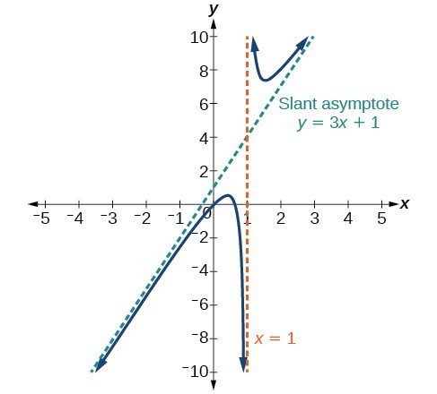
Figure 13. Slant Asymptote when [latex]f\left(x\right)=\frac{p\left(x\right)}{q\left(x\right)},q\left(x\right)\ne 0\\[/latex] where degree of [latex]p>\text{ degree of }q\text{ by }1\\[/latex].
Case 3: If the degree of the denominator = degree of the numerator, there is a horizontal asymptote at [latex]y=\frac{{a}_{n}}{{b}_{n}}\\[/latex], where [latex]{a}_{n}[/latex] and [latex]{b}_{n}\\[/latex] are the leading coefficients of [latex]p\left(x\right)\\[/latex] and [latex]q\left(x\right)\\[/latex] for [latex]f\left(x\right)=\frac{p\left(x\right)}{q\left(x\right)},q\left(x\right)\ne 0\\[/latex].
In this case, the end behavior is [latex]f\left(x\right)\approx \frac{3{x}^{2}}{{x}^{2}}=3\\[/latex]. This tells us that as the inputs grow large, this function will behave like the function [latex]g\left(x\right)=3\\[/latex], which is a horizontal line. As [latex]x\to \pm \infty ,f\left(x\right)\to 3\\[/latex], resulting in a horizontal asymptote at y = 3. Note that this graph crosses the horizontal asymptote.
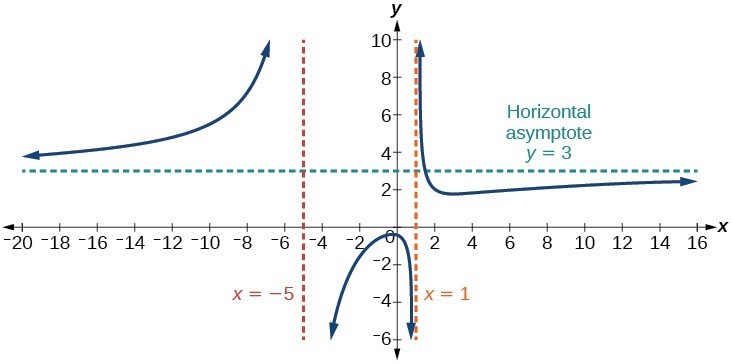
Figure 14. Horizontal Asymptote when [latex]f\left(x\right)=\frac{p\left(x\right)}{q\left(x\right)},q\left(x\right)\ne 0\text{where degree of }p=\text{degree of }q\\[/latex].
Notice that, while the graph of a rational function will never cross a vertical asymptote, the graph may or may not cross a horizontal or slant asymptote. Also, although the graph of a rational function may have many vertical asymptotes, the graph will have at most one horizontal (or slant) asymptote.
It should be noted that, if the degree of the numerator is larger than the degree of the denominator by more than one, the end behavior of the graph will mimic the behavior of the reduced end behavior fraction. For instance, if we had the function
with end behavior
the end behavior of the graph would look similar to that of an even polynomial with a positive leading coefficient.
The horizontal asymptote of a rational function can be determined by looking at the degrees of the numerator and denominator.
For the functions below, identify the horizontal or slant asymptote.
For these solutions, we will use [latex]f\left(x\right)=\frac{p\left(x\right)}{q\left(x\right)}, q\left(x\right)\ne 0\\[/latex].

[latex]k\left(x\right)=\frac{{x}^{2}+4x}{{x}^{3}-8}\\[/latex]: The degree of [latex]p=2\text{ }<\\[/latex] degree of [latex]q=3\\[/latex], so there is a horizontal asymptote y = 0.
In the sugar concentration problem earlier, we created the equation [latex]C\left(t\right)=\frac{5+t}{100+10t}\\[/latex].
Find the horizontal asymptote and interpret it in context of the problem.
Both the numerator and denominator are linear (degree 1). Because the degrees are equal, there will be a horizontal asymptote at the ratio of the leading coefficients. In the numerator, the leading term is t, with coefficient 1. In the denominator, the leading term is 10t, with coefficient 10. The horizontal asymptote will be at the ratio of these values:
This function will have a horizontal asymptote at [latex]y=\frac{1}{10}\\[/latex].
This tells us that as the values of t increase, the values of C will approach [latex]\frac{1}{10}\\[/latex]. In context, this means that, as more time goes by, the concentration of sugar in the tank will approach one-tenth of a pound of sugar per gallon of water or [latex]\frac{1}{10}\\[/latex] pounds per gallon.
Find the horizontal and vertical asymptotes of the function
First, note that this function has no common factors, so there are no potential removable discontinuities.
The function will have vertical asymptotes when the denominator is zero, causing the function to be undefined. The denominator will be zero at [latex]x=1,-2,\text{and }5\\[/latex], indicating vertical asymptotes at these values.
The numerator has degree 2, while the denominator has degree 3. Since the degree of the denominator is greater than the degree of the numerator, the denominator will grow faster than the numerator, causing the outputs to tend towards zero as the inputs get large, and so as [latex]x\to \pm \infty , f\left(x\right)\to 0\\[/latex]. This function will have a horizontal asymptote at [latex]y=0\\[/latex].
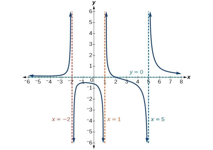
Figure 15
Find the vertical and horizontal asymptotes of the function:
[latex]f\left(x\right)=\frac{\left(2x - 1\right)\left(2x+1\right)}{\left(x - 2\right)\left(x+3\right)}\\[/latex]
A rational function will have a y-intercept when the input is zero, if the function is defined at zero. A rational function will not have a y-intercept if the function is not defined at zero.
Likewise, a rational function will have x-intercepts at the inputs that cause the output to be zero. Since a fraction is only equal to zero when the numerator is zero, x-intercepts can only occur when the numerator of the rational function is equal to zero.
Find the intercepts of [latex]f\left(x\right)=\frac{\left(x - 2\right)\left(x+3\right)}{\left(x - 1\right)\left(x+2\right)\left(x - 5\right)}\\[/latex].
We can find the y-intercept by evaluating the function at zero
The x-intercepts will occur when the function is equal to zero:
The y-intercept is [latex]\left(0,-0.6\right)\\[/latex], the x-intercepts are [latex]\left(2,0\right)\\[/latex] and [latex]\left(-3,0\right)\\[/latex].
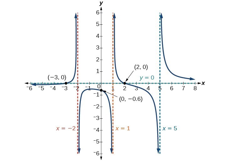
Figure 16
Given the reciprocal squared function that is shifted right 3 units and down 4 units, write this as a rational function. Then, find the x– and y-intercepts and the horizontal and vertical asymptotes.
While vertical asymptotes describe the behavior of a graph as the output gets very large or very small, horizontal asymptotes help describe the behavior of a graph as the input gets very large or very small. Recall that a polynomial’s end behavior will mirror that of the leading term. Likewise, a rational function’s end behavior will mirror that of the ratio of the leading terms of the numerator and denominator functions.
There are three distinct outcomes when checking for horizontal asymptotes:
Case 1: If the degree of the denominator > degree of the numerator, there is a horizontal asymptote at y = 0.
In this case, the end behavior is [latex]fleft(xright)approx frac{4x}{{x}^{2}}=frac{4}{x}\[/latex]. This tells us that, as the inputs increase or decrease without bound, this function will behave similarly to the function [latex]gleft(xright)=frac{4}{x}\[/latex], and the outputs will approach zero, resulting in a horizontal asymptote at y = 0. Note that this graph crosses the horizontal asymptote.
Figure 12. Horizontal Asymptote y = 0 when [latex]fleft(xright)=frac{pleft(xright)}{qleft(xright)},qleft(xright)ne{0}text{ where degree of }p<text{degree of q}\[/latex].
Case 2: If the degree of the denominator < degree of the numerator by one, we get a slant asymptote.
In this case, the end behavior is [latex]fleft(xright)approx frac{3{x}^{2}}{x}=3x\[/latex]. This tells us that as the inputs increase or decrease without bound, this function will behave similarly to the function [latex]gleft(xright)=3x\[/latex]. As the inputs grow large, the outputs will grow and not level off, so this graph has no horizontal asymptote. However, the graph of [latex]gleft(xright)=3x\[/latex] looks like a diagonal line, and since f will behave similarly to g, it will approach a line close to [latex]y=3x\[/latex]. This line is a slant asymptote.
To find the equation of the slant asymptote, divide [latex]frac{3{x}^{2}-2x+1}{x - 1}\[/latex]. The quotient is [latex]3x+1\[/latex], and the remainder is 2. The slant asymptote is the graph of the line [latex]gleft(xright)=3x+1\[/latex].
Figure 13. Slant Asymptote when [latex]fleft(xright)=frac{pleft(xright)}{qleft(xright)},qleft(xright)ne 0\[/latex] where degree of [latex]p>text{ degree of }qtext{ by }1\[/latex].
Case 3: If the degree of the denominator = degree of the numerator, there is a horizontal asymptote at [latex]y=frac{{a}_{n}}{{b}_{n}}\[/latex], where [latex]{a}_{n}[/latex] and [latex]{b}_{n}\[/latex] are the leading coefficients of [latex]pleft(xright)\[/latex] and [latex]qleft(xright)\[/latex] for [latex]fleft(xright)=frac{pleft(xright)}{qleft(xright)},qleft(xright)ne 0\[/latex].
In this case, the end behavior is [latex]fleft(xright)approx frac{3{x}^{2}}{{x}^{2}}=3\[/latex]. This tells us that as the inputs grow large, this function will behave like the function [latex]gleft(xright)=3\[/latex], which is a horizontal line. As [latex]xto pm infty ,fleft(xright)to 3\[/latex], resulting in a horizontal asymptote at y = 3. Note that this graph crosses the horizontal asymptote.
Figure 14. Horizontal Asymptote when [latex]fleft(xright)=frac{pleft(xright)}{qleft(xright)},qleft(xright)ne 0text{where degree of }p=text{degree of }q\[/latex].
Notice that, while the graph of a rational function will never cross a vertical asymptote, the graph may or may not cross a horizontal or slant asymptote. Also, although the graph of a rational function may have many vertical asymptotes, the graph will have at most one horizontal (or slant) asymptote.
It should be noted that, if the degree of the numerator is larger than the degree of the denominator by more than one, the end behavior of the graph will mimic the behavior of the reduced end behavior fraction. For instance, if we had the function
with end behavior
the end behavior of the graph would look similar to that of an even polynomial with a positive leading coefficient.
The horizontal asymptote of a rational function can be determined by looking at the degrees of the numerator and denominator.
For the functions below, identify the horizontal or slant asymptote.
For these solutions, we will use [latex]fleft(xright)=frac{pleft(xright)}{qleft(xright)}, qleft(xright)ne 0\[/latex].
The quotient is [latex]x - 2\[/latex] and the remainder is 13. There is a slant asymptote at [latex]y=-x - 2\[/latex].
In the sugar concentration problem earlier, we created the equation [latex]Cleft(tright)=frac{5+t}{100+10t}\[/latex].
Find the horizontal asymptote and interpret it in context of the problem.
Both the numerator and denominator are linear (degree 1). Because the degrees are equal, there will be a horizontal asymptote at the ratio of the leading coefficients. In the numerator, the leading term is t, with coefficient 1. In the denominator, the leading term is 10t, with coefficient 10. The horizontal asymptote will be at the ratio of these values:
This function will have a horizontal asymptote at [latex]y=frac{1}{10}\[/latex].
This tells us that as the values of t increase, the values of C will approach [latex]frac{1}{10}\[/latex]. In context, this means that, as more time goes by, the concentration of sugar in the tank will approach one-tenth of a pound of sugar per gallon of water or [latex]frac{1}{10}\[/latex] pounds per gallon.
Find the horizontal and vertical asymptotes of the function
First, note that this function has no common factors, so there are no potential removable discontinuities.
The function will have vertical asymptotes when the denominator is zero, causing the function to be undefined. The denominator will be zero at [latex]x=1,-2,text{and }5\[/latex], indicating vertical asymptotes at these values.
The numerator has degree 2, while the denominator has degree 3. Since the degree of the denominator is greater than the degree of the numerator, the denominator will grow faster than the numerator, causing the outputs to tend towards zero as the inputs get large, and so as [latex]xto pm infty , fleft(xright)to 0\[/latex]. This function will have a horizontal asymptote at [latex]y=0\[/latex].
Figure 15
Find the vertical and horizontal asymptotes of the function:
[latex]fleft(xright)=frac{left(2x - 1right)left(2x+1right)}{left(x - 2right)left(x+3right)}\[/latex]
A rational function will have a y-intercept when the input is zero, if the function is defined at zero. A rational function will not have a y-intercept if the function is not defined at zero.
Likewise, a rational function will have x-intercepts at the inputs that cause the output to be zero. Since a fraction is only equal to zero when the numerator is zero, x-intercepts can only occur when the numerator of the rational function is equal to zero.
Find the intercepts of [latex]fleft(xright)=frac{left(x - 2right)left(x+3right)}{left(x - 1right)left(x+2right)left(x - 5right)}\[/latex].
We can find the y-intercept by evaluating the function at zero
The x-intercepts will occur when the function is equal to zero:
The y-intercept is [latex]left(0,-0.6right)\[/latex], the x-intercepts are [latex]left(2,0right)\[/latex] and [latex]left(-3,0right)\[/latex].
Figure 16
Given the reciprocal squared function that is shifted right 3 units and down 4 units, write this as a rational function. Then, find the x– and y-intercepts and the horizontal and vertical asymptotes.
In Example 9, we see that the numerator of a rational function reveals the x-intercepts of the graph, whereas the denominator reveals the vertical asymptotes of the graph. As with polynomials, factors of the numerator may have integer powers greater than one. Fortunately, the effect on the shape of the graph at those intercepts is the same as we saw with polynomials.
The vertical asymptotes associated with the factors of the denominator will mirror one of the two toolkit reciprocal functions. When the degree of the factor in the denominator is odd, the distinguishing characteristic is that on one side of the vertical asymptote the graph heads towards positive infinity, and on the other side the graph heads towards negative infinity.
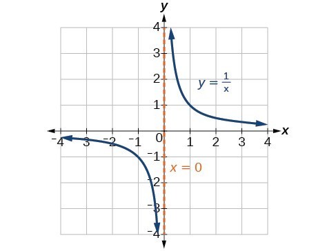
Figure 17
When the degree of the factor in the denominator is even, the distinguishing characteristic is that the graph either heads toward positive infinity on both sides of the vertical asymptote or heads toward negative infinity on both sides.
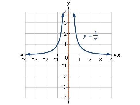
Figure 18
For example, the graph of [latex]f\left(x\right)=\frac{{\left(x+1\right)}^{2}\left(x - 3\right)}{{\left(x+3\right)}^{2}\left(x - 2\right)}\\[/latex] is shown in Figure 19.
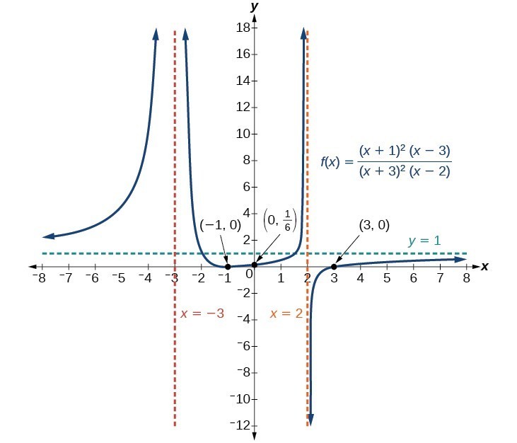
Figure 19
Sketch a graph of [latex]f\left(x\right)=\frac{\left(x+2\right)\left(x - 3\right)}{{\left(x+1\right)}^{2}\left(x - 2\right)}\\[/latex].
We can start by noting that the function is already factored, saving us a step.
Next, we will find the intercepts. Evaluating the function at zero gives the y-intercept:
To find the x-intercepts, we determine when the numerator of the function is zero. Setting each factor equal to zero, we find x-intercepts at [latex]x=-2\\[/latex] and [latex]x=3\\[/latex]. At each, the behavior will be linear (multiplicity 1), with the graph passing through the intercept.
We have a y-intercept at [latex]\left(0,3\right)\\[/latex] and x-intercepts at [latex]\left(-2,0\right)\\[/latex] and [latex]\left(3,0\right)\\[/latex].
To find the vertical asymptotes, we determine when the denominator is equal to zero. This occurs when [latex]x+1=0\\[/latex] and when [latex]x - 2=0\\[/latex], giving us vertical asymptotes at [latex]x=-1\\[/latex] and [latex]x=2\\[/latex].
There are no common factors in the numerator and denominator. This means there are no removable discontinuities.
Finally, the degree of denominator is larger than the degree of the numerator, telling us this graph has a horizontal asymptote at [latex]y=0\\[/latex].
To sketch the graph, we might start by plotting the three intercepts. Since the graph has no x-intercepts between the vertical asymptotes, and the y-intercept is positive, we know the function must remain positive between the asymptotes, letting us fill in the middle portion of the graph as shown in Figure 20.
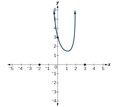
Figure 20
The factor associated with the vertical asymptote at [latex]x=-1\\[/latex] was squared, so we know the behavior will be the same on both sides of the asymptote. The graph heads toward positive infinity as the inputs approach the asymptote on the right, so the graph will head toward positive infinity on the left as well.
For the vertical asymptote at [latex]x=2\\[/latex], the factor was not squared, so the graph will have opposite behavior on either side of the asymptote. After passing through the x-intercepts, the graph will then level off toward an output of zero, as indicated by the horizontal asymptote.
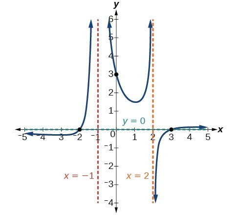
Figure 21
Given the function [latex]f\left(x\right)=\frac{{\left(x+2\right)}^{2}\left(x - 2\right)}{2{\left(x - 1\right)}^{2}\left(x - 3\right)}\\[/latex], use the characteristics of polynomials and rational functions to describe its behavior and sketch the function.
Now that we have analyzed the equations for rational functions and how they relate to a graph of the function, we can use information given by a graph to write the function. A rational function written in factored form will have an x-intercept where each factor of the numerator is equal to zero. (An exception occurs in the case of a removable discontinuity.) As a result, we can form a numerator of a function whose graph will pass through a set of x-intercepts by introducing a corresponding set of factors. Likewise, because the function will have a vertical asymptote where each factor of the denominator is equal to zero, we can form a denominator that will produce the vertical asymptotes by introducing a corresponding set of factors.
If a rational function has x-intercepts at [latex]x={x}_{1}, {x}_{2}, …, {x}_{n}\\[/latex], vertical asymptotes at [latex]x={v}_{1},{v}_{2},\dots ,{v}_{m}\\[/latex], and no [latex]{x}_{i}=\text{any }{v}_{j}\\[/latex], then the function can be written in the form:
where the powers [latex]{p}_{i}\\[/latex] or [latex]{q}_{i}\\[/latex] on each factor can be determined by the behavior of the graph at the corresponding intercept or asymptote, and the stretch factor a can be determined given a value of the function other than the x-intercept or by the horizontal asymptote if it is nonzero.
Write an equation for the rational function shown in Figure 22.
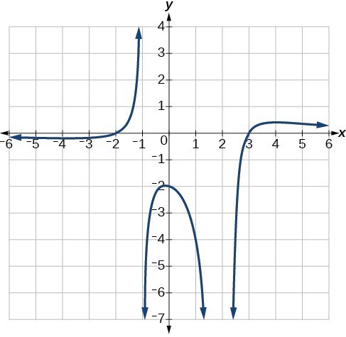
Figure 22
The graph appears to have x-intercepts at [latex]x=-2\\[/latex] and [latex]x=3\\[/latex]. At both, the graph passes through the intercept, suggesting linear factors. The graph has two vertical asymptotes. The one at [latex]x=-1\\[/latex] seems to exhibit the basic behavior similar to [latex]\frac{1}{x}\\[/latex], with the graph heading toward positive infinity on one side and heading toward negative infinity on the other. The asymptote at [latex]x=2\\[/latex] is exhibiting a behavior similar to [latex]\frac{1}{{x}^{2}}\\[/latex], with the graph heading toward negative infinity on both sides of the asymptote.
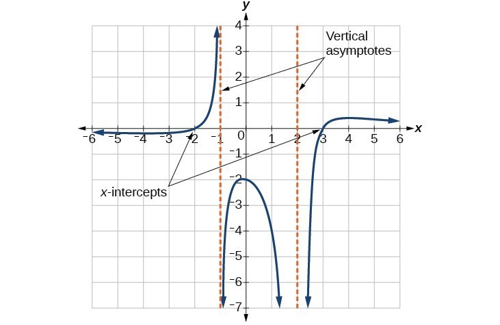
Figure 23
We can use this information to write a function of the form
To find the stretch factor, we can use another clear point on the graph, such as the y-intercept [latex]\left(0,-2\right)\\[/latex].
This gives us a final function of [latex]f\left(x\right)=\frac{4\left(x+2\right)\left(x - 3\right)}{3\left(x+1\right){\left(x - 2\right)}^{2}}\\[/latex].
| Rational Function | [latex]f\left(x\right)=\frac{P\left(x\right)}{Q\left(x\right)}=\frac{{a}_{p}{x}^{p}+{a}_{p - 1}{x}^{p - 1}+…+{a}_{1}x+{a}_{0}}{{b}_{q}{x}^{q}+{b}_{q - 1}{x}^{q - 1}+…+{b}_{1}x+{b}_{0}}, Q\left(x\right)\ne 0[/latex] |
1. What is the fundamental difference in the algebraic representation of a polynomial function and a rational function?
2. What is the fundamental difference in the graphs of polynomial functions and rational functions?
3. If the graph of a rational function has a removable discontinuity, what must be true of the functional rule?
4. Can a graph of a rational function have no vertical asymptote? If so, how?
5. Can a graph of a rational function have no x-intercepts? If so, how?
For the following exercises, find the domain of the rational functions.
6. [latex]f\left(x\right)=\frac{x - 1}{x+2}\\[/latex]
7. [latex]f\left(x\right)=\frac{x+1}{{x}^{2}-1}\\[/latex]
8. [latex]f\left(x\right)=\frac{{x}^{2}+4}{{x}^{2}-2x - 8}\\[/latex]
9. [latex]f\left(x\right)=\frac{{x}^{2}+4x - 3}{{x}^{4}-5{x}^{2}+4}\\[/latex]
For the following exercises, find the domain, vertical asymptotes, and horizontal asymptotes of the functions.
10. [latex]f\left(x\right)=\frac{4}{x - 1}\\[/latex]
11. [latex]f\left(x\right)=\frac{2}{5x+2}\\[/latex]
12. [latex]f\left(x\right)=\frac{x}{{x}^{2}-9}\\[/latex]
13. [latex]f\left(x\right)=\frac{x}{{x}^{2}+5x - 36}\\[/latex]
14. [latex]f\left(x\right)=\frac{3+x}{{x}^{3}-27}\\[/latex]
15. [latex]f\left(x\right)=\frac{3x - 4}{{x}^{3}-16x}\\[/latex]
16. [latex]f\left(x\right)=\frac{{x}^{2}-1}{{x}^{3}+9{x}^{2}+14x}\\[/latex]
17. [latex]f\left(x\right)=\frac{x+5}{{x}^{2}-25}\\[/latex]
18. [latex]f\left(x\right)=\frac{x - 4}{x - 6}\\[/latex]
19. [latex]f\left(x\right)=\frac{4 - 2x}{3x - 1}\\[/latex]
For the following exercises, find the x– and y-intercepts for the functions.
20. [latex]f\left(x\right)=\frac{x+5}{{x}^{2}+4}\\[/latex]
21. [latex]f\left(x\right)=\frac{x}{{x}^{2}-x}\\[/latex]
22. [latex]f\left(x\right)=\frac{{x}^{2}+8x+7}{{x}^{2}+11x+30}\\[/latex]
23. [latex]f\left(x\right)=\frac{{x}^{2}+x+6}{{x}^{2}-10x+24}\\[/latex]
24. [latex]f\left(x\right)=\frac{94 - 2{x}^{2}}{3{x}^{2}-12}\\[/latex]
For the following exercises, describe the local and end behavior of the functions.
25. [latex]f\left(x\right)=\frac{x}{2x+1}\\[/latex]
26. [latex]f\left(x\right)=\frac{2x}{x - 6}\\[/latex]
27. [latex]f\left(x\right)=\frac{-2x}{x - 6}\\[/latex]
28. [latex]f\left(x\right)=\frac{{x}^{2}-4x+3}{{x}^{2}-4x - 5}\\[/latex]
29. [latex]f\left(x\right)=\frac{2{x}^{2}-32}{6{x}^{2}+13x - 5}\\[/latex]
For the following exercises, find the slant asymptote of the functions.
30. [latex]f\left(x\right)=\frac{24{x}^{2}+6x}{2x+1}\\[/latex]
31. [latex]f\left(x\right)=\frac{4{x}^{2}-10}{2x - 4}\\[/latex]
32. [latex]f\left(x\right)=\frac{81{x}^{2}-18}{3x - 2}\\[/latex]
33. [latex]f\left(x\right)=\frac{6{x}^{3}-5x}{3{x}^{2}+4}\\[/latex]
34. [latex]f\left(x\right)=\frac{{x}^{2}+5x+4}{x - 1}\\[/latex]
For the following exercises, use the given transformation to graph the function. Note the vertical and horizontal asymptotes.
35. The reciprocal function shifted up two units.
36. The reciprocal function shifted down one unit and left three units.
37. The reciprocal squared function shifted to the right 2 units.
38. The reciprocal squared function shifted down 2 units and right 1 unit.
For the following exercises, find the horizontal intercepts, the vertical intercept, the vertical asymptotes, and the horizontal or slant asymptote of the functions. Use that information to sketch a graph.
39. [latex]p\left(x\right)=\frac{2x - 3}{x+4}\\[/latex]
40. [latex]q\left(x\right)=\frac{x - 5}{3x - 1}\\[/latex]
41. [latex]s\left(x\right)=\frac{4}{{\left(x - 2\right)}^{2}}\\[/latex]
42. [latex]r\left(x\right)=\frac{5}{{\left(x+1\right)}^{2}}\\[/latex]
43. [latex]f\left(x\right)=\frac{3{x}^{2}-14x - 5}{3{x}^{2}+8x - 16}\\[/latex]
44. [latex]g\left(x\right)=\frac{2{x}^{2}+7x - 15}{3{x}^{2}-14+15}\\[/latex]
45. [latex]a\left(x\right)=\frac{{x}^{2}+2x - 3}{{x}^{2}-1}\\[/latex]
46. [latex]b\left(x\right)=\frac{{x}^{2}-x - 6}{{x}^{2}-4}\\[/latex]
47. [latex]h\left(x\right)=\frac{2{x}^{2}+ x - 1}{x - 4}\\[/latex]
48. [latex]k\left(x\right)=\frac{2{x}^{2}-3x - 20}{x - 5}\\[/latex]
49. [latex]w\left(x\right)=\frac{\left(x - 1\right)\left(x+3\right)\left(x - 5\right)}{{\left(x+2\right)}^{2}\left(x - 4\right)}\\[/latex]
50. [latex]z\left(x\right)=\frac{{\left(x+2\right)}^{2}\left(x - 5\right)}{\left(x - 3\right)\left(x+1\right)\left(x+4\right)}\\[/latex]
For the following exercises, write an equation for a rational function with the given characteristics.
51. Vertical asymptotes at x = 5 and x = –5, x-intercepts at [latex]\left(2,0\right)\\[/latex] and [latex]\left(-1,0\right)\\[/latex], y-intercept at [latex]\left(0,4\right)\\[/latex]
52. Vertical asymptotes at [latex]x=-4\\[/latex] and [latex]x=-1\\[/latex], x-intercepts at [latex]\left(1,0\right)\\[/latex] and [latex]\left(5,0\right)\\[/latex], y-intercept at [latex]\left(0,7\right)\\[/latex]
53. Vertical asymptotes at [latex]x=-4\\[/latex] and [latex]x=-5\\[/latex], x-intercepts at [latex]\left(4,0\right)\\[/latex] and [latex]\left(-6,0\right)\\[/latex], Horizontal asymptote at [latex]y=7\\[/latex]
54. Vertical asymptotes at [latex]x=-3\\[/latex] and [latex]x=6\\[/latex], x-intercepts at [latex]\left(-2,0\right)\\[/latex] and [latex]\left(1,0\right)\\[/latex], Horizontal asymptote at [latex]y=-2\\[/latex]
55. Vertical asymptote at [latex]x=-1\\[/latex], Double zero at [latex]x=2\\[/latex], y-intercept at [latex]\left(0,2\right)\\[/latex]
56. Vertical asymptote at [latex]x=3\\[/latex], Double zero at [latex]x=1\\[/latex], y-intercept at [latex]\left(0,4\right)\\[/latex]
For the following exercises, use the graphs to write an equation for the function.
57.
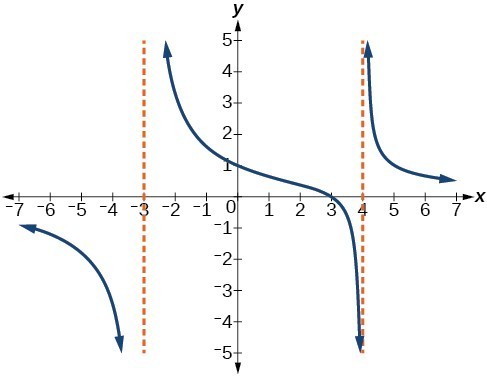
58.
59.
60.
61.
62.
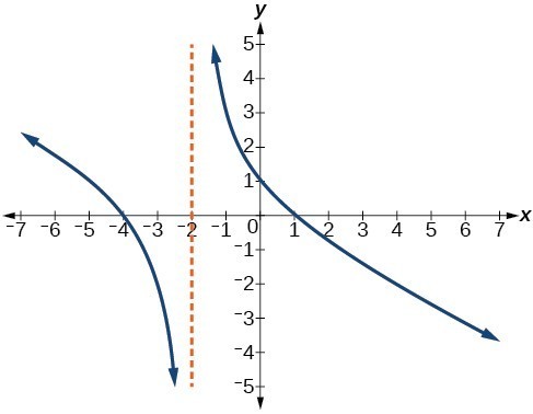
63.
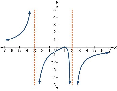
64.
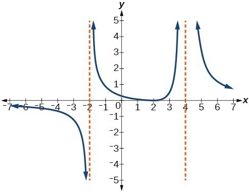
For the following exercises, make tables to show the behavior of the function near the vertical asymptote and reflecting the horizontal asymptote
65. [latex]f\left(x\right)=\frac{1}{x - 2}\\[/latex]
66. [latex]f\left(x\right)=\frac{x}{x - 3}\\[/latex]
67. [latex]f\left(x\right)=\frac{2x}{x+4}\\[/latex]
68. [latex]f\left(x\right)=\frac{2x}{{\left(x - 3\right)}^{2}}\\[/latex]
69. [latex]f\left(x\right)=\frac{{x}^{2}}{{x}^{2}+2x+1}\\[/latex]
For the following exercises, use a calculator to graph [latex]f\left(x\right)\\[/latex]. Use the graph to solve [latex]f\left(x\right)>0\\[/latex].
70. [latex]f\left(x\right)=\frac{2}{x+1}\\[/latex]
71. [latex]f\left(x\right)=\frac{4}{2x - 3}\\[/latex]
72. [latex]f\left(x\right)=\frac{2}{\left(x - 1\right)\left(x+2\right)}\\[/latex]
73. [latex]f\left(x\right)=\frac{x+2}{\left(x - 1\right)\left(x - 4\right)}\\[/latex]
74. [latex]f\left(x\right)=\frac{{\left(x+3\right)}^{2}}{{\left(x - 1\right)}^{2}\left(x+1\right)}\\[/latex]
For the following exercises, identify the removable discontinuity.
75. [latex]f\left(x\right)=\frac{{x}^{2}-4}{x - 2}\\[/latex]
76. [latex]f\left(x\right)=\frac{{x}^{3}+1}{x+1}\\[/latex]
77. [latex]f\left(x\right)=\frac{{x}^{2}+x - 6}{x - 2}\\[/latex]
78. [latex]f\left(x\right)=\frac{2{x}^{2}+5x - 3}{x+3}\\[/latex]
79. [latex]f\left(x\right)=\frac{{x}^{3}+{x}^{2}}{x+1}\\[/latex]
For the following exercises, express a rational function that describes the situation.
80. A large mixing tank currently contains 200 gallons of water, into which 10 pounds of sugar have been mixed. A tap will open, pouring 10 gallons of water per minute into the tank at the same time sugar is poured into the tank at a rate of 3 pounds per minute. Find the concentration (pounds per gallon) of sugar in the tank after t minutes.
81. A large mixing tank currently contains 300 gallons of water, into which 8 pounds of sugar have been mixed. A tap will open, pouring 20 gallons of water per minute into the tank at the same time sugar is poured into the tank at a rate of 2 pounds per minute. Find the concentration (pounds per gallon) of sugar in the tank after t minutes.
For the following exercises, use the given rational function to answer the question.
82. The concentration C of a drug in a patient’s bloodstream t hours after injection in given by [latex]C\left(t\right)=\frac{2t}{3+{t}^{2}}\\[/latex]. What happens to the concentration of the drug as t increases?
83. The concentration C of a drug in a patient’s bloodstream t hours after injection is given by [latex]C\left(t\right)=\frac{100t}{2{t}^{2}+75}\\[/latex]. Use a calculator to approximate the time when the concentration is highest.
For the following exercises, construct a rational function that will help solve the problem. Then, use a calculator to answer the question.
84. An open box with a square base is to have a volume of 108 cubic inches. Find the dimensions of the box that will have minimum surface area. Let x = length of the side of the base.
85. A rectangular box with a square base is to have a volume of 20 cubic feet. The material for the base costs 30 cents/ square foot. The material for the sides costs 10 cents/square foot. The material for the top costs 20 cents/square foot. Determine the dimensions that will yield minimum cost. Let x = length of the side of the base.
86. A right circular cylinder has volume of 100 cubic inches. Find the radius and height that will yield minimum surface area. Let x = radius.
87. A right circular cylinder with no top has a volume of 50 cubic meters. Find the radius that will yield minimum surface area. Let x = radius.
88. A right circular cylinder is to have a volume of 40 cubic inches. It costs 4 cents/square inch to construct the top and bottom and 1 cent/square inch to construct the rest of the cylinder. Find the radius to yield minimum cost. Let x = radius.
1. End behavior: as [latex]x\to \pm \infty , f\left(x\right)\to 0\\[/latex]; Local behavior: as [latex]x\to 0, f\left(x\right)\to \infty \\[/latex] (there are no x– or y-intercepts)
2. The function and the asymptotes are shifted 3 units right and 4 units down. As [latex]x\to 3,f\left(x\right)\to \infty\\ [/latex], and as [latex]x\to \pm \infty ,f\left(x\right)\to -4\\[/latex].
The function is [latex]f\left(x\right)=\frac{1}{{\left(x - 3\right)}^{2}}-4\\[/latex].

3. [latex]\frac{12}{11}\\[/latex]
4. The domain is all real numbers except [latex]x=1\\[/latex] and [latex]x=5\\[/latex].
5. Removable discontinuity at [latex]x=5\\[/latex]. Vertical asymptotes: [latex]x=0,\text{ }x=1\\[/latex].
6. Vertical asymptotes at [latex]x=2\\[/latex] and [latex]x=-3\\[/latex]; horizontal asymptote at [latex]y=4\\[/latex].
7. For the transformed reciprocal squared function, we find the rational form. [latex]f\left(x\right)=\frac{1}{{\left(x - 3\right)}^{2}}-4=\frac{1 - 4{\left(x - 3\right)}^{2}}{{\left(x - 3\right)}^{2}}=\frac{1 - 4\left({x}^{2}-6x+9\right)}{\left(x - 3\right)\left(x - 3\right)}=\frac{-4{x}^{2}+24x - 35}{{x}^{2}-6x+9}\\[/latex]
Because the numerator is the same degree as the denominator we know that as [latex]x\to \pm \infty , f\left(x\right)\to -4; \text{so } y=-4\\[/latex] is the horizontal asymptote. Next, we set the denominator equal to zero, and find that the vertical asymptote is [latex]x=3\\[/latex], because as [latex]x\to 3,f\left(x\right)\to \infty \\[/latex]. We then set the numerator equal to 0 and find the x-intercepts are at [latex]\left(2.5,0\right)\\[/latex] and [latex]\left(3.5,0\right)\\[/latex]. Finally, we evaluate the function at 0 and find the y-intercept to be at [latex]\left(0,\frac{-35}{9}\right)\\[/latex].
8. Horizontal asymptote at [latex]y=\frac{1}{2}\\[/latex]. Vertical asymptotes at [latex]x=1 \text{and} x=3\\[/latex]. y-intercept at [latex]\left(0,\frac{4}{3}.\right)\\[/latex]
x-intercepts at [latex]\left(2,0\right) \text{ and }\left(-2,0\right)\\[/latex]. [latex]\left(-2,0\right)\\[/latex] is a zero with multiplicity 2, and the graph bounces off the x-axis at this point. [latex]\left(2,0\right)\\[/latex] is a single zero and the graph crosses the axis at this point.
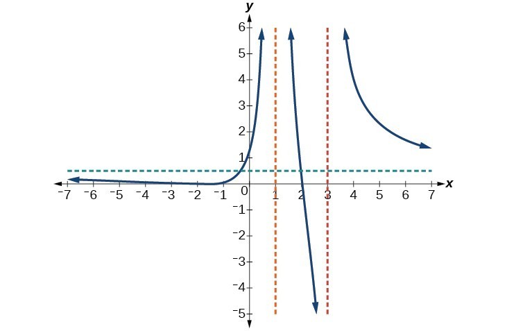
1. The rational function will be represented by a quotient of polynomial functions.
3. The numerator and denominator must have a common factor.
5. Yes. The numerator of the formula of the functions would have only complex roots and/or factors common to both the numerator and denominator.
7. [latex]\text{All reals }x\ne -1, 1\\[/latex]
9. [latex]\text{All reals }x\ne -1, -2, 1, 2\\[/latex]
11. V.A. at [latex]x=-\frac{2}{5}\\[/latex]; H.A. at [latex]y=0\\[/latex]; Domain is all reals [latex]x\ne -\frac{2}{5}\\[/latex]
13. V.A. at [latex]x=4, -9\\[/latex]; H.A. at [latex]y=0\\[/latex]; Domain is all reals [latex]x\ne 4, -9\\[/latex]
15. V.A. at [latex]x=0, 4, -4\\[/latex]; H.A. at [latex]y=0\\[/latex]; Domain is all reals [latex]x\ne 0,4, -4\\[/latex]
17. V.A. at [latex]x=-5\\[/latex]; H.A. at [latex]y=0\\[/latex]; Domain is all reals [latex]x\ne 5,-5\\[/latex]
19. V.A. at [latex]x=\frac{1}{3}\\[/latex]; H.A. at [latex]y=-\frac{2}{3}\\[/latex]; Domain is all reals [latex]x\ne \frac{1}{3}\\[/latex].
21. none
23. [latex]x\text{-intercepts none, }y\text{-intercept }\left(0,\frac{1}{4}\right)\\[/latex]
25. Local behavior: [latex]x\to -{\frac{1}{2}}^{+},f\left(x\right)\to -\infty ,x\to -{\frac{1}{2}}^{-},f\left(x\right)\to \infty \\[/latex]
End behavior: [latex]x\to \pm \infty ,f\left(x\right)\to \frac{1}{2}\\[/latex]
27. Local behavior: [latex]x\to {6}^{+},f\left(x\right)\to -\infty ,x\to {6}^{-},f\left(x\right)\to \infty \\[/latex], End behavior: [latex]x\to \pm \infty ,f\left(x\right)\to -2\\[/latex]
29. Local behavior: [latex]x\to -{\frac{1}{3}}^{+},f\left(x\right)\to \infty ,x\to -{\frac{1}{3}}^{-}\\[/latex], [latex]f\left(x\right)\to -\infty ,x\to {\frac{5}{2}}^{-},f\left(x\right)\to \infty ,x\to {\frac{5}{2}}^{+}\\[/latex] , [latex]f\left(x\right)\to -\infty \\[/latex]
End behavior: [latex]x\to \pm \infty\\ [/latex], [latex]f\left(x\right)\to \frac{1}{3}\\[/latex]
31. [latex]y=2x+4\\[/latex]
33. [latex]y=2x\\[/latex]
35. [latex]V.A.\text{ }x=0,H.A.\text{ }y=2\\[/latex]
37. [latex]V.A.\text{ }x=2,\text{ }H.A.\text{ }y=0\\[/latex]

39. [latex]V.A.\text{ }x=-4,\text{ }H.A.\text{ }y=2;\left(\frac{3}{2},0\right);\left(0,-\frac{3}{4}\right)\\[/latex]

41. [latex]V.A.\text{ }x=2,\text{ }H.A.\text{ }y=0,\text{ }\left(0,1\right)\\[/latex]

43. [latex]V.A.\text{ }x=-4,\text{ }x=\frac{4}{3},\text{ }H.A.\text{ }y=1;\left(5,0\right);\left(-\frac{1}{3},0\right);\left(0,\frac{5}{16}\right)\\[/latex]
45. [latex]V.A.\text{ }x=-1,\text{ }H.A.\text{ }y=1;\left(-3,0\right);\left(0,3\right)\\[/latex]

47. [latex]V.A.\text{ }x=4,\text{ }S.A.\text{ }y=2x+9;\left(-1,0\right);\left(\frac{1}{2},0\right);\left(0,\frac{1}{4}\right)\\[/latex]

49. [latex]V.A.\text{ }x=-2,\text{ }x=4,\text{ }H.A.\text{ }y=1,\left(1,0\right);\left(5,0\right);\left(-3,0\right);\left(0,-\frac{15}{16}\right)\\[/latex]

51. [latex]y=50\frac{{x}^{2}-x - 2}{{x}^{2}-25}\\[/latex]
53. [latex]y=7\frac{{x}^{2}+2x - 24}{{x}^{2}+9x+20}\\[/latex]
55. [latex]y=\frac{1}{2}\frac{{x}^{2}-4x+4}{x+1}\\[/latex]
57. [latex]y=4\frac{x - 3}{{x}^{2}-x - 12}\\[/latex]
59. [latex]y=-9\frac{x - 2}{{x}^{2}-9}\\[/latex]
61. [latex]y=\frac{1}{3}\frac{{x}^{2}+x - 6}{x - 1}\\[/latex]
63. [latex]y=-6\frac{{\left(x - 1\right)}^{2}}{\left(x+3\right){\left(x - 2\right)}^{2}}\\[/latex]
65.
| x | 2.01 | 2.001 | 2.0001 | 1.99 | 1.999 |
| y | 100 | 1,000 | 10,000 | –100 | –1,000 |
| x | 10 | 100 | 1,000 | 10,000 | 100,000 |
| y | .125 | .0102 | .001 | .0001 | .00001 |
Vertical asymptote [latex]x=2\\[/latex], Horizontal asymptote [latex]y=0\\[/latex]
67.
| x | –4.1 | –4.01 | –4.001 | –3.99 | –3.999 |
| y | 82 | 802 | 8,002 | –798 | –7998 |
| x | 10 | 100 | 1,000 | 10,000 | 100,000 |
| y | 1.4286 | 1.9331 | 1.992 | 1.9992 | 1.999992 |
Vertical asymptote [latex]x=-4\\[/latex], Horizontal asymptote [latex]y=2\\[/latex]
69.
| x | –.9 | –.99 | –.999 | –1.1 | –1.01 |
| y | 81 | 9,801 | 998,001 | 121 | 10,201 |
| x | 10 | 100 | 1,000 | 10,000 | 100,000 |
| y | .82645 | .9803 | .998 | .9998 |
Vertical asymptote [latex]x=-1\\[/latex], Horizontal asymptote [latex]y=1\\[/latex]
71. [latex]\left(\frac{3}{2},\infty \right)\\[/latex]

73. [latex]\left(-2,1\right)\cup \left(4,\infty \right)\\[/latex]

75. [latex]\left(2,4\right)\\[/latex]
77. [latex]\left(2,5\right)\\[/latex]
79. [latex]\left(-1,\text{1}\right)\\[/latex]
81. [latex]C\left(t\right)=\frac{8+2t}{300+20t}\\[/latex]
83. After about 6.12 hours.
85. [latex]A\left(x\right)=50{x}^{2}+\frac{800}{x}\\[/latex]. 2 by 2 by 5 feet.
87. [latex]A\left(x\right)=\pi {x}^{2}+\frac{100}{x}\\[/latex]. Radius = 2.52 meters.
By the end of this lesson, you will be able to:
Figure 1
A mound of gravel is in the shape of a cone with the height equal to twice the radius.
The volume is found using a formula from elementary geometry.
We have written the volume V in terms of the radius r. However, in some cases, we may start out with the volume and want to find the radius. For example: A customer purchases 100 cubic feet of gravel to construct a cone shape mound with a height twice the radius. What are the radius and height of the new cone? To answer this question, we use the formula
This function is the inverse of the formula for V in terms of r.
In this section, we will explore the inverses of polynomial and rational functions and in particular the radical functions we encounter in the process.
Two functions f and g are inverse functions if for every coordinate pair in f, (a, b), there exists a corresponding coordinate pair in the inverse function, g, (b, a). In other words, the coordinate pairs of the inverse functions have the input and output interchanged.
For a function to have an inverse function the function to create a new function that is one-to-one and would have an inverse function.
For example, suppose a water runoff collector is built in the shape of a parabolic trough as shown below. We can use the information in the figure to find the surface area of the water in the trough as a function of the depth of the water.
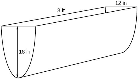
Figure 2
Because it will be helpful to have an equation for the parabolic cross-sectional shape, we will impose a coordinate system at the cross section, with x measured horizontally and y measured vertically, with the origin at the vertex of the parabola.
Figure 3
From this we find an equation for the parabolic shape. We placed the origin at the vertex of the parabola, so we know the equation will have form [latex]y\left(x\right)=a{x}^{2}\\[/latex]. Our equation will need to pass through the point (6, 18), from which we can solve for the stretch factor a.
Our parabolic cross section has the equation
We are interested in the surface area of the water, so we must determine the width at the top of the water as a function of the water depth. For any depth y the width will be given by 2x, so we need to solve the equation above for x and find the inverse function. However, notice that the original function is not one-to-one, and indeed, given any output there are two inputs that produce the same output, one positive and one negative.
To find an inverse, we can restrict our original function to a limited domain on which it is one-to-one. In this case, it makes sense to restrict ourselves to positive x values. On this domain, we can find an inverse by solving for the input variable:
This is not a function as written. We are limiting ourselves to positive x values, so we eliminate the negative solution, giving us the inverse function we’re looking for.
Because x is the distance from the center of the parabola to either side, the entire width of the water at the top will be 2x. The trough is 3 feet (36 inches) long, so the surface area will then be:
This example illustrates two important points:
Functions involving roots are often called radical functions. While it is not possible to find an inverse of most polynomial functions, some basic polynomials do have inverses. Such functions are called invertible functions, and we use the notation [latex]{f}^{-1}\left(x\right)\\[/latex].
Warning: [latex]{f}^{-1}\left(x\right)\\[/latex] is not the same as the reciprocal of the function [latex]f\left(x\right)\\[/latex]. This use of –1 is reserved to denote inverse functions. To denote the reciprocal of a function [latex]f\left(x\right)\\[/latex], we would need to write [latex]{\left(f\left(x\right)\right)}^{-1}=\frac{1}{f\left(x\right)}\\[/latex].
An important relationship between inverse functions is that they “undo” each other. If [latex]{f}^{-1}\\[/latex] is the inverse of a function f, then f is the inverse of the function [latex]{f}^{-1}\\[/latex]. In other words, whatever the function f does to x, [latex]{f}^{-1}\\[/latex] undoes it—and vice-versa. More formally, we write
and
Two functions, f and g, are inverses of one another if for all x in the domain of f and g.
Show that [latex]f\left(x\right)=\frac{1}{x+1}\\[/latex] and [latex]{f}^{-1}\left(x\right)=\frac{1}{x}-1\\[/latex] are inverses, for [latex]x\ne 0,-1\\[/latex] .
We must show that [latex]{f}^{-1}\left(f\left(x\right)\right)=x\\[/latex] and [latex]f\left({f}^{-1}\left(x\right)\right)=x\\[/latex].
Therefore, [latex]f\left(x\right)=\frac{1}{x+1}\\[/latex] and [latex]{f}^{-1}\left(x\right)=\frac{1}{x}-1\\[/latex] are inverses.
Show that [latex]f\left(x\right)=\frac{x+5}{3}\\[/latex] and [latex]{f}^{-1}\left(x\right)=3x - 5\\[/latex] are inverses.
Find the inverse of the function [latex]f\left(x\right)=5{x}^{3}+1\\[/latex].
This is a transformation of the basic cubic toolkit function, and based on our knowledge of that function, we know it is one-to-one. Solving for the inverse by solving for x.
Look at the graph of f and [latex]{f}^{-1}\\[/latex]. Notice that the two graphs are symmetrical about the line [latex]y=x\\[/latex]. This is always the case when graphing a function and its inverse function.
Also, since the method involved interchanging x and y, notice corresponding points. If [latex]\left(a,b\right)\\[/latex] is on the graph of f, then [latex]\left(b,a\right)\\[/latex] is on the graph of [latex]{f}^{-1}\\[/latex]. Since [latex]\left(0,1\right)\\[/latex] is on the graph of f, then [latex]\left(1,0\right)\\[/latex] is on the graph of [latex]{f}^{-1}\\[/latex]. Similarly, since [latex]\left(1,6\right)\\[/latex] is on the graph of f, then [latex]\left(6,1\right)\\[/latex] is on the graph of [latex]{f}^{-1}\\[/latex].
Figure 4
So far, we have been able to find the inverse functions of cubic functions without having to restrict their domains. However, as we know, not all cubic polynomials are one-to-one. Some functions that are not one-to-one may have their domain restricted so that they are one-to-one, but only over that domain. The function over the restricted domain would then have an inverse function. Since quadratic functions are not one-to-one, we must restrict their domain in order to find their inverses.
If a function is not one-to-one, it cannot have an inverse. If we restrict the domain of the function so that it becomes one-to-one, thus creating a new function, this new function will have an inverse.
Find the inverse function of f:
The original function [latex]f\left(x\right)={\left(x - 4\right)}^{2}\\[/latex] is not one-to-one, but the function is restricted to a domain of [latex]x\ge 4\\[/latex] or [latex]x\le 4\\[/latex] on which it is one-to-one.
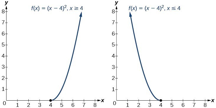
Figure 5
To find the inverse, start by replacing [latex]f\left(x\right)\\[/latex] with the simple variable y.
This is not a function as written. We need to examine the restrictions on the domain of the original function to determine the inverse. Since we reversed the roles of x and y for the original f(x), we looked at the domain: the values x could assume. When we reversed the roles of x and y, this gave us the values y could assume. For this function, [latex]x\ge 4\\[/latex], so for the inverse, we should have [latex]y\ge 4\\[/latex], which is what our inverse function gives.
On the graphs below, we see the original function graphed on the same set of axes as its inverse function. Notice that together the graphs show symmetry about the line [latex]y=x\\[/latex]. The coordinate pair [latex]\left(4, 0\right)\\[/latex] is on the graph of f and the coordinate pair [latex]\left(0, 4\right)\\[/latex] is on the graph of [latex]{f}^{-1}\\[/latex]. For any coordinate pair, if (a, b) is on the graph of f, then (b, a) is on the graph of [latex]{f}^{-1}\\[/latex]. Finally, observe that the graph of f intersects the graph of [latex]{f}^{-1}\\[/latex] on the line y = x. Points of intersection for the graphs of f and [latex]{f}^{-1}\\[/latex] will always lie on the line y = x.
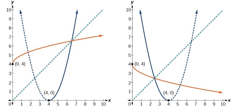
Figure 6
Restrict the domain and then find the inverse of
We can see this is a parabola with vertex at [latex]\left(2, -3\right)\\[/latex] that opens upward. Because the graph will be decreasing on one side of the vertex and increasing on the other side, we can restrict this function to a domain on which it will be one-to-one by limiting the domain to [latex]x\ge 2\\[/latex].
To find the inverse, we will use the vertex form of the quadratic. We start by replacing f(x) with a simple variable, y, then solve for x.
Now we need to determine which case to use. Because we restricted our original function to a domain of [latex]x\ge 2\\[/latex], the outputs of the inverse should be the same, telling us to utilize the + case
If the quadratic had not been given in vertex form, rewriting it into vertex form would be the first step. This way we may easily observe the coordinates of the vertex to help us restrict the domain.
Notice that we arbitrarily decided to restrict the domain on [latex]x\ge 2\\[/latex]. We could just have easily opted to restrict the domain on [latex]x\le 2\\[/latex], in which case [latex]{f}^{-1}\left(x\right)=2-\sqrt{x+3}\\[/latex]. Observe the original function graphed on the same set of axes as its inverse function in the graph below. Notice that both graphs show symmetry about the line y = x. The coordinate pair [latex]\left(2,\text{ }-3\right)\\[/latex] is on the graph of f and the coordinate pair [latex]\left(-3,\text{ }2\right)\\[/latex] is on the graph of [latex]{f}^{-1}\\[/latex]. Observe from the graph of both functions on the same set of axes that
and
Finally, observe that the graph of f intersects the graph of [latex]{f}^{-1}\\[/latex] along the line y = x.
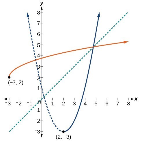
Figure 7
Find the inverse of the function [latex]f\left(x\right)={x}^{2}+1\\[/latex], on the domain [latex]x\ge 0\\[/latex].
Notice that the functions from previous examples were all polynomials, and their inverses were radical functions. If we want to find the inverse of a radical function, we will need to restrict the domain of the answer because the range of the original function is limited.
Restrict the domain and then find the inverse of the function [latex]f\left(x\right)=\sqrt{x - 4}\\[/latex].
Note that the original function has range [latex]f\left(x\right)\ge 0\\[/latex]. Replace [latex]f\left(x\right)\\[/latex] with y, then solve for x.
Recall that the domain of this function must be limited to the range of the original function.
Notice in the graph below that the inverse is a reflection of the original function over the line y = x. Because the original function has only positive outputs, the inverse function has only positive inputs.
Figure 8
Restrict the domain and then find the inverse of the function [latex]f\left(x\right)=\sqrt{2x+3}\\[/latex].
Radical functions are common in physical models, as we saw in the section opener. We now have enough tools to be able to solve the problem posed at the start of the section.
A mound of gravel is in the shape of a cone with the height equal to twice the radius. The volume of the cone in terms of the radius is given by
Find the inverse of the function [latex]V=\frac{2}{3}\pi {r}^{3}\\[/latex] that determines the volume V of a cone and is a function of the radius r. Then use the inverse function to calculate the radius of such a mound of gravel measuring 100 cubic feet. Use [latex]\pi =3.14\\[/latex].
Start with the given function for V. Notice that the meaningful domain for the function is [latex]r\ge 0\\[/latex] since negative radii would not make sense in this context. Also note the range of the function (hence, the domain of the inverse function) is [latex]V\ge 0\\[/latex]. Solve for r in terms of V, using the method outlined previously.
This is the result stated in the section opener. Now evaluate this for V = 100 and [latex]\pi =3.14\\[/latex].
Therefore, the radius is about 3.63 ft.
When radical functions are composed with other functions, determining domain can become more complicated.
Find the domain of the function [latex]f\left(x\right)=\sqrt{\frac{\left(x+2\right)\left(x - 3\right)}{\left(x - 1\right)}}\\[/latex].
Because a square root is only defined when the quantity under the radical is non-negative, we need to determine where [latex]\frac{\left(x+2\right)\left(x - 3\right)}{\left(x - 1\right)}\ge 0\\[/latex]. The output of a rational function can change signs (change from positive to negative or vice versa) at x-intercepts and at vertical asymptotes. For this equation, the graph could change signs at x = –2, 1, and 3.
To determine the intervals on which the rational expression is positive, we could test some values in the expression or sketch a graph. While both approaches work equally well, for this example we will use a graph.
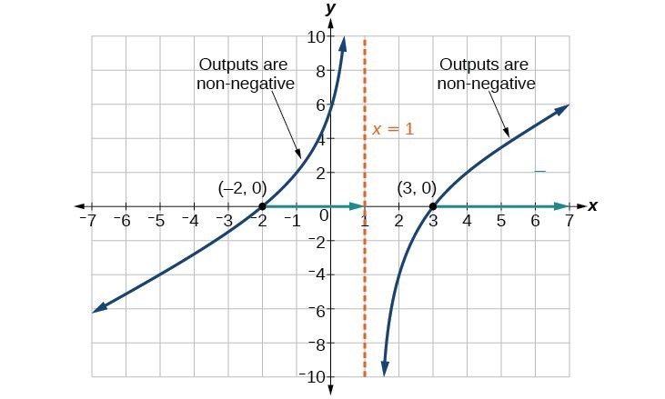
Figure 9
This function has two x-intercepts, both of which exhibit linear behavior near the x-intercepts. There is one vertical asymptote, corresponding to a linear factor; this behavior is similar to the basic reciprocal toolkit function, and there is no horizontal asymptote because the degree of the numerator is larger than the degree of the denominator. There is a y-intercept at (0, 6).
From the y-intercept and x-intercept at x = –2, we can sketch the left side of the graph. From the behavior at the asymptote, we can sketch the right side of the graph.
From the graph, we can now tell on which intervals the outputs will be non-negative, so that we can be sure that the original function f(x) will be defined. f(x) has domain [latex]-2\le x<1\text{or}x\ge 3\\[/latex], or in interval notation, [latex]\left[-2,1\right)\cup \left[3,\infty \right)\\[/latex].
As with finding inverses of quadratic functions, it is sometimes desirable to find the inverse of a rational function, particularly of rational functions that are the ratio of linear functions, such as in concentration applications.
The function [latex]C=\frac{20+0.4n}{100+n}\\[/latex] represents the concentration C of an acid solution after n mL of 40% solution has been added to 100 mL of a 20% solution. First, find the inverse of the function; that is, find an expression for n in terms of C. Then use your result to determine how much of the 40% solution should be added so that the final mixture is a 35% solution.
We first want the inverse of the function. We will solve for n in terms of C.
Now evaluate this function for C=0.35 (35%).
We can conclude that 300 mL of the 40% solution should be added.
Find the inverse of the function [latex]f\left(x\right)=\frac{x+3}{x - 2}\\[/latex].
1. Explain why we cannot find inverse functions for all polynomial functions.
2. Why must we restrict the domain of a quadratic function when finding its inverse?
3. When finding the inverse of a radical function, what restriction will we need to make?
4. The inverse of a quadratic function will always take what form?
For the following exercises, find the inverse of the function on the given domain.
5. [latex]f\left(x\right)={\left(x - 4\right)}^{2}, \left[4,\infty \right)\\[/latex]
6. [latex]f\left(x\right)={\left(x+2\right)}^{2}, \left[-2,\infty \right)\\[/latex]
7. [latex]f\left(x\right)={\left(x+1\right)}^{2}-3, \left[-1,\infty \right)\\[/latex]
8. [latex]f\left(x\right)=2-\sqrt{3+x}\\[/latex]
9. [latex]f\left(x\right)=3{x}^{2}+5,\left(-\infty ,0\right],\left[0,\infty \right)\\[/latex]
10. [latex]f\left(x\right)=12-{x}^{2}, \left[0,\infty \right)\\[/latex]
11. [latex]f\left(x\right)=9-{x}^{2}, \left[0,\infty \right)\\[/latex]
12. [latex]f\left(x\right)=2{x}^{2}+4, \left[0,\infty \right)\\[/latex]
For the following exercises, find the inverse of the functions.
13. [latex]f\left(x\right)={x}^{3}+5\\[/latex]
14. [latex]f\left(x\right)=3{x}^{3}+1\\[/latex]
15. [latex]f\left(x\right)=4-{x}^{3}\\[/latex]
16. [latex]f\left(x\right)=4 - 2{x}^{3}\\[/latex]
For the following exercises, find the inverse of the functions.
17. [latex]f\left(x\right)=\sqrt{2x+1}\\[/latex]
18. [latex]f\left(x\right)=\sqrt{3 - 4x}\\[/latex]
19. [latex]f\left(x\right)=9+\sqrt{4x - 4}\\[/latex]
20. [latex]f\left(x\right)=\sqrt{6x - 8}+5\\[/latex]
21. [latex]f\left(x\right)=9+2\sqrt[3]{x}\\[/latex]
22. [latex]f\left(x\right)=3-\sqrt[3]{x}\\[/latex]
23. [latex]f\left(x\right)=\frac{2}{x+8}\\[/latex]
24. [latex]f\left(x\right)=\frac{3}{x - 4}\\[/latex]
25. [latex]f\left(x\right)=\frac{x+3}{x+7}\\[/latex]
26. [latex]f\left(x\right)=\frac{x - 2}{x+7}\\[/latex]
27. [latex]f\left(x\right)=\frac{3x+4}{5 - 4x}\\[/latex]
28. [latex]f\left(x\right)=\frac{5x+1}{2 - 5x}\\[/latex]
29. [latex]f\left(x\right)={x}^{2}+2x, \left[-1,\infty \right)\\[/latex]
30. [latex]f\left(x\right)={x}^{2}+4x+1, \left[-2,\infty \right)\\[/latex]
31. [latex]f\left(x\right)={x}^{2}-6x+3, \left[3,\infty \right)\\[/latex]
For the following exercises, find the inverse of the function and graph both the function and its inverse.
32. [latex]f\left(x\right)={x}^{2}+2,x\ge 0\\[/latex]
33. [latex]f\left(x\right)=4-{x}^{2},x\ge 0\\[/latex]
34. [latex]f\left(x\right)={\left(x+3\right)}^{2},x\ge -3\\[/latex]
35. [latex]f\left(x\right)={\left(x - 4\right)}^{2},x\ge 4\\[/latex]
36. [latex]f\left(x\right)={x}^{3}+3\\[/latex]
37. [latex]f\left(x\right)=1-{x}^{3}\\[/latex]
38. [latex]f\left(x\right)={x}^{2}+4x,x\ge -2\\[/latex]
39. [latex]f\left(x\right)={x}^{2}-6x+1,x\ge 3\\[/latex]
40. [latex]f\left(x\right)=\frac{2}{x}\\[/latex]
41. [latex]f\left(x\right)=\frac{1}{{x}^{2}},x\ge 0\\[/latex]
For the following exercises, use a graph to help determine the domain of the functions.
42. [latex]f\left(x\right)=\sqrt{\frac{\left(x+1\right)\left(x - 1\right)}{x}}\\[/latex]
43. [latex]f\left(x\right)=\sqrt{\frac{\left(x+2\right)\left(x - 3\right)}{x - 1}}\\[/latex]
44. [latex]f\left(x\right)=\sqrt{\frac{x\left(x+3\right)}{x - 4}}\\[/latex]
45. [latex]f\left(x\right)=\sqrt{\frac{{x}^{2}-x - 20}{x - 2}}\\[/latex]
46. [latex]f\left(x\right)=\sqrt{\frac{9-{x}^{2}}{x+4}}\\[/latex]
For the following exercises, use a calculator to graph the function. Then, using the graph, give three points on the graph of the inverse with y-coordinates given.
47. [latex]f\left(x\right)={x}^{3}-x - 2,y=1, 2, 3\\[/latex]
48. [latex]f\left(x\right)={x}^{3}+x - 2, y=0, 1, 2\\[/latex]
49. [latex]f\left(x\right)={x}^{3}+3x - 4, y=0, 1, 2\\[/latex]
50. [latex]f\left(x\right)={x}^{3}+8x - 4, y=-1, 0, 1\\[/latex]
51. [latex]f\left(x\right)={x}^{4}+5x+1, y=-1, 0, 1\\[/latex]
For the following exercises, find the inverse of the functions with a, b, c positive real numbers.
52. [latex]f\left(x\right)=a{x}^{3}+b\\[/latex]
53. [latex]f\left(x\right)={x}^{2}+bx\\[/latex]
54. [latex]f\left(x\right)=\sqrt{a{x}^{2}+b}\\[/latex]
55. [latex]f\left(x\right)=\sqrt[3]{ax+b}\\[/latex]
56. [latex]f\left(x\right)=\frac{ax+b}{x+c}\\[/latex]
For the following exercises, determine the function described and then use it to answer the question.
57. An object dropped from a height of 200 meters has a height, [latex]h\left(t\right)\\[/latex], in meters after t seconds have lapsed, such that [latex]h\left(t\right)=200 - 4.9{t}^{2}\\[/latex]. Express t as a function of height, h, and find the time to reach a height of 50 meters.
58. An object dropped from a height of 600 feet has a height, [latex]h\left(t\right)\\[/latex], in feet after t seconds have elapsed, such that [latex]h\left(t\right)=600 - 16{t}^{2}\\[/latex]. Express t as a function of height h, and find the time to reach a height of 400 feet.
59. The volume, V, of a sphere in terms of its radius, r, is given by [latex]V\left(r\right)=\frac{4}{3}\pi {r}^{3}\\[/latex]. Express r as a function of V, and find the radius of a sphere with volume of 200 cubic feet.
60. The surface area, A, of a sphere in terms of its radius, r, is given by [latex]A\left(r\right)=4\pi {r}^{2}\\[/latex]. Express r as a function of V, and find the radius of a sphere with a surface area of 1000 square inches.
61. A container holds 100 ml of a solution that is 25 ml acid. If n ml of a solution that is 60% acid is added, the function [latex]C\left(n\right)=\frac{25+.6n}{100+n}\\[/latex] gives the concentration, C, as a function of the number of ml added, n. Express n as a function of C and determine the number of mL that need to be added to have a solution that is 50% acid.
62. The period T, in seconds, of a simple pendulum as a function of its length l, in feet, is given by [latex]T\left(l\right)=2\pi \sqrt{\frac{l}{32.2}}\\[/latex]. Express l as a function of T and determine the length of a pendulum with period of 2 seconds.
63. The volume of a cylinder, V, in terms of radius, r, and height, h, is given by [latex]V=\pi {r}^{2}h\\[/latex]. If a cylinder has a height of 6 meters, express the radius as a function of V and find the radius of a cylinder with volume of 300 cubic meters.
64. The surface area, A, of a cylinder in terms of its radius, r, and height, h, is given by [latex]A=2\pi {r}^{2}+2\pi rh\\[/latex]. If the height of the cylinder is 4 feet, express the radius as a function of V and find the radius if the surface area is 200 square feet.
65. The volume of a right circular cone, V, in terms of its radius, r, and its height, h, is given by [latex]V=\frac{1}{3}\pi {r}^{2}h\\[/latex]. Express r in terms of h if the height of the cone is 12 feet and find the radius of a cone with volume of 50 cubic inches.
66. Consider a cone with height of 30 feet. Express the radius, r, in terms of the volume, V, and find the radius of a cone with volume of 1000 cubic feet.
1. [latex]{f}^{-1}\left(f\left(x\right)\right)={f}^{-1}\left(\frac{x+5}{3}\right)=3\left(\frac{x+5}{3}\right)-5=\left(x - 5\right)+5=x\\[/latex] and [latex]f\left({f}^{-1}\left(x\right)\right)=f\left(3x - 5\right)=\frac{\left(3x - 5\right)+5}{3}=\frac{3x}{3}=x\\[/latex]
2. [latex]{f}^{-1}\left(x\right)={x}^{3}-4\\[/latex]
3. [latex]{f}^{-1}\left(x\right)=\sqrt{x - 1}\\[/latex]
4. [latex]{f}^{-1}\left(x\right)=\frac{{x}^{2}-3}{2},x\ge 0\\[/latex]
5. [latex]{f}^{-1}\left(x\right)=\frac{2x+3}{x - 1}\\[/latex]
1. It can be too difficult or impossible to solve for x in terms of y.
3. We will need a restriction on the domain of the answer.
5. [latex]{f}^{-1}\left(x\right)=\sqrt{x}+4\\[/latex]
7. [latex]{f}^{-1}\left(x\right)=\sqrt{x+3}-1\\[/latex]
9. [latex]{f}^{-1}\left(x\right)=-\sqrt{\frac{x - 5}{3}}\\[/latex]
11. [latex]f\left(x\right)=\sqrt{9-x}\\[/latex]
13. [latex]{f}^{-1}\left(x\right)=\sqrt[3]{x - 5}\\[/latex]
15. [latex]{f}^{-1}\left(x\right)=\sqrt[3]{4-x}\\[/latex]
17. [latex]{f}^{-1}\left(x\right)=\frac{{x}^{2}-1}{2},\left[0,\infty \right)\\[/latex]
19. [latex]{f}^{-1}\left(x\right)=\frac{{\left(x - 9\right)}^{2}+4}{4},\left[9,\infty \right)\\[/latex]
21. [latex]{f}^{-1}\left(x\right)={\left(\frac{x - 9}{2}\right)}^{3}\\[/latex]
23. [latex]{f}^{-1}\left(x\right)={\frac{2 - 8x}{x}}\\[/latex]
25. [latex]{f}^{-1}\left(x\right)=\frac{7x - 3}{1-x}\\[/latex]
27. [latex]{f}^{-1}\left(x\right)=\frac{5x - 4}{4x+3}\\[/latex]
29. [latex]{f}^{-1}\left(x\right)=\sqrt{x+1}-1\\[/latex]
31. [latex]{f}^{-1}\left(x\right)=\sqrt{x+6}+3\\[/latex]
33. [latex]{f}^{-1}\left(x\right)=\sqrt{4-x}\\[/latex]

35. [latex]{f}^{-1}\left(x\right)=\sqrt{x}+4\\[/latex]
37. [latex]{f}^{-1}\left(x\right)=\sqrt[3]{1-x}\\[/latex]

39. [latex]{f}^{-1}\left(x\right)=\sqrt{x+8}+3\\[/latex]

41. [latex]{f}^{-1}\left(x\right)=\sqrt{\frac{1}{x}}\\[/latex]

43. [latex]\left[-2,1\right)\cup \left[3,\infty \right)\\[/latex]
45. [latex]\left[-4,2\right)\cup \left[5,\infty \right)\\[/latex]

47. [latex]\left(-2, 0\right); \left(4, 2\right); \left(22, 3\right)\\[/latex]

49. [latex]\left(-4, 0\right); \left(0, 1\right); \left(10, 2\right)\\[/latex]
51. [latex]\left(-3, -1\right); \left(1, 0\right); \left(7, 1\right)\\[/latex]
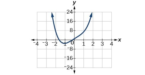
53. [latex]{f}^{-1}\left(x\right)=\sqrt{x+\frac{{b}^{2}}{4}}-\frac{b}{2}\\[/latex]
55. [latex]{f}^{-1}\left(x\right)=\frac{{x}^{3}-b}{a}\\[/latex]
57. [latex]t\left(h\right)=\sqrt{\frac{200-h}{4.9}}\\[/latex], 5.53 seconds
59. [latex]r\left(V\right)=\sqrt[3]{\frac{3V}{4\pi }}\\[/latex], 3.63 feet
61. [latex]n\left(C\right)=\frac{100C - 25}{.6-C}\\[/latex], 250 mL
63. [latex]r\left(V\right)=\sqrt{\frac{V}{6\pi }}\\[/latex], 3.99 meters
65. [latex]r\left(V\right)=\sqrt{\frac{V}{4\pi }}\\[/latex], 1.99 inches

Figure 1. Electron micrograph of E.Coli bacteria (credit: “Mattosaurus,” Wikimedia Commons)
Focus in on a square centimeter of your skin. Look closer. Closer still. If you could look closely enough, you would see hundreds of thousands of microscopic organisms. They are bacteria, and they are not only on your skin, but in your mouth, nose, and even your intestines. In fact, the bacterial cells in your body at any given moment outnumber your own cells. But that is no reason to feel bad about yourself. While some bacteria can cause illness, many are healthy and even essential to the body.
Bacteria commonly reproduce through a process called binary fission, during which one bacterial cell splits into two. When conditions are right, bacteria can reproduce very quickly. Unlike humans and other complex organisms, the time required to form a new generation of bacteria is often a matter of minutes or hours, as opposed to days or years. (Todar, PhD, Kenneth. Todar's Online Textbook of Bacteriology. http://textbookofbacteriology.net/growth_3.html.)
For simplicity’s sake, suppose we begin with a culture of one bacterial cell that can divide every hour. The table below shows the number of bacterial cells at the end of each subsequent hour. We see that the single bacterial cell leads to over one thousand bacterial cells in just ten hours! And if we were to extrapolate the table to twenty-four hours, we would have over 16 million!
| Hour | 0 | 1 | 2 | 3 | 4 | 5 | 6 | 7 | 8 | 9 | 10 |
| Bacteria | 1 | 2 | 4 | 8 | 16 | 32 | 64 | 128 | 256 | 512 | 1024 |
In this chapter, we will explore exponential functions, which can be used for, among other things, modeling growth patterns such as those found in bacteria. We will also investigate logarithmic functions, which are closely related to exponential functions. Both types of functions have numerous real-world applications when it comes to modeling and interpreting data.
By the end of this lesson, you will be able to:
India is the second most populous country in the world with a population of about 1.25 billion people in 2013. The population is growing at a rate of about 1.2% each year. (http://www.worldometers.info/world-population/. Accessed February 24, 2014.) If this rate continues, the population of India will exceed China’s population by the year 2031. When populations grow rapidly, we often say that the growth is “exponential,” meaning that something is growing very rapidly. To a mathematician, however, the term exponential growth has a very specific meaning. In this section, we will take a look at exponential functions, which model this kind of rapid growth.
Recall that the base of an exponential function must be a positive real number other than 1. Why do we limit the base b to positive values? To ensure that the outputs will be real numbers. Observe what happens if the base is not positive:
Why do we limit the base to positive values other than 1? Because base 1 results in the constant function. Observe what happens if the base is 1:
To evaluate an exponential function with the form [latex]f\left(x\right)={b}^{x}\\[/latex], we simply substitute x with the given value, and calculate the resulting power. For example:
Let [latex]f\left(x\right)={2}^{x}\\[/latex]. What is [latex]f\left(3\right)\\[/latex]?
To evaluate an exponential function with a form other than the basic form, it is important to follow the order of operations. For example:
Let [latex]f\left(x\right)=30{\left(2\right)}^{x}\\[/latex]. What is [latex]f\left(3\right)\\[/latex]?
Note that if the order of operations were not followed, the result would be incorrect:
Let [latex]f\left(x\right)=5{\left(3\right)}^{x+1}\\[/latex]. Evaluate [latex]f\left(2\right)\\[/latex] without using a calculator.
Follow the order of operations. Be sure to pay attention to the parentheses.
Let [latex]f\left(x\right)=8{\left(1.2\right)}^{x - 5}\\[/latex]. Evaluate [latex]f\left(3\right)\\[/latex] using a calculator. Round to four decimal places.
Because the output of exponential functions increases very rapidly, the term “exponential growth” is often used in everyday language to describe anything that grows or increases rapidly. However, exponential growth can be defined more precisely in a mathematical sense. If the growth rate is proportional to the amount present, the function models exponential growth.
A function that models exponential growth grows by a rate proportional to the amount present. For any real number x and any positive real numbers a and b such that [latex]b\ne 1\\[/latex], an exponential growth function has the form
where
In more general terms, we have an exponential function, in which a constant base is raised to a variable exponent. To differentiate between linear and exponential functions, let’s consider two companies, A and B. Company A has 100 stores and expands by opening 50 new stores a year, so its growth can be represented by the function [latex]A\left(x\right)=100+50x\\[/latex]. Company B has 100 stores and expands by increasing the number of stores by 50% each year, so its growth can be represented by the function [latex]B\left(x\right)=100{\left(1+0.5\right)}^{x}\\[/latex].
A few years of growth for these companies are illustrated below.
| Year, x | Stores, Company A | Stores, Company B |
|---|---|---|
| 0 | 100 + 50(0) = 100 | 100(1 + 0.5)0 = 100 |
| 1 | 100 + 50(1) = 150 | 100(1 + 0.5)1 = 150 |
| 2 | 100 + 50(2) = 200 | 100(1 + 0.5)2 = 225 |
| 3 | 100 + 50(3) = 250 | 100(1 + 0.5)3 = 337.5 |
| x | A(x) = 100 + 50x | B(x) = 100(1 + 0.5)x |
The graphs comparing the number of stores for each company over a five-year period are shown in below. We can see that, with exponential growth, the number of stores increases much more rapidly than with linear growth.
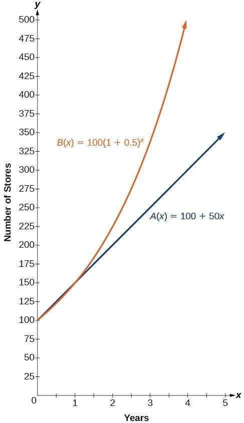
Figure 2. The graph shows the numbers of stores Companies A and B opened over a five-year period.
Notice that the domain for both functions is [latex]\left[0,\infty \right)\\[/latex], and the range for both functions is [latex]\left[100,\infty \right)\\[/latex]. After year 1, Company B always has more stores than Company A.
Now we will turn our attention to the function representing the number of stores for Company B, [latex]B\left(x\right)=100{\left(1+0.5\right)}^{x}\\[/latex]. In this exponential function, 100 represents the initial number of stores, 0.50 represents the growth rate, and [latex]1+0.5=1.5\\[/latex] represents the growth factor. Generalizing further, we can write this function as [latex]B\left(x\right)=100{\left(1.5\right)}^{x}\\[/latex], where 100 is the initial value, 1.5 is called the base, and x is called the exponent.
At the beginning of this section, we learned that the population of India was about 1.25 billion in the year 2013, with an annual growth rate of about 1.2%. This situation is represented by the growth function [latex]P\left(t\right)=1.25{\left(1.012\right)}^{t}\\[/latex], where t is the number of years since 2013. To the nearest thousandth, what will the population of India be in 2031?
To estimate the population in 2031, we evaluate the models for t = 18, because 2031 is 18 years after 2013. Rounding to the nearest thousandth,
There will be about 1.549 billion people in India in the year 2031.
The population of China was about 1.39 billion in the year 2013, with an annual growth rate of about 0.6%. This situation is represented by the growth function [latex]P\left(t\right)=1.39{\left(1.006\right)}^{t}\\[/latex], where t is the number of years since 2013. To the nearest thousandth, what will the population of China be for the year 2031? How does this compare to the population prediction we made for India in Example 2?
In the previous examples, we were given an exponential function, which we then evaluated for a given input. Sometimes we are given information about an exponential function without knowing the function explicitly. We must use the information to first write the form of the function, then determine the constants a and b, and evaluate the function.
In 2006, 80 deer were introduced into a wildlife refuge. By 2012, the population had grown to 180 deer. The population was growing exponentially. Write an algebraic function N(t) representing the population N of deer over time t.
We let our independent variable t be the number of years after 2006. Thus, the information given in the problem can be written as input-output pairs: (0, 80) and (6, 180). Notice that by choosing our input variable to be measured as years after 2006, we have given ourselves the initial value for the function, a = 80. We can now substitute the second point into the equation [latex]N\left(t\right)=80{b}^{t}\\[/latex] to find b:
NOTE: Unless otherwise stated, do not round any intermediate calculations. Then round the final answer to four places for the remainder of this section.
The exponential model for the population of deer is [latex]N\left(t\right)=80{\left(1.1447\right)}^{t}\\[/latex]. (Note that this exponential function models short-term growth. As the inputs gets large, the output will get increasingly larger, so much so that the model may not be useful in the long term.)
We can graph our model to observe the population growth of deer in the refuge over time. Notice that the graph below passes through the initial points given in the problem, [latex]\left(0,\text{ 8}0\right)\\[/latex] and [latex]\left(\text{6},\text{ 18}0\right)\\[/latex]. We can also see that the domain for the function is [latex]\left[0,\infty \right)\\[/latex], and the range for the function is [latex]\left[80,\infty \right)\\[/latex].
Figure 3. Graph showing the population of deer over time, [latex]N\left(t\right)=80{\left(1.1447\right)}^{t}\\[/latex], t years after 2006
A wolf population is growing exponentially. In 2011, 129 wolves were counted. By 2013 the population had reached 236 wolves. What two points can be used to derive an exponential equation modeling this situation? Write the equation representing the population N of wolves over time t.
Find an exponential function that passes through the points [latex]\left(-2,6\right)\\[/latex] and [latex]\left(2,1\right)\\[/latex].
Because we don’t have the initial value, we substitute both points into an equation of the form [latex]f\left(x\right)=a{b}^{x}\\[/latex], and then solve the system for a and b.
Use the first equation to solve for a in terms of b:
Substitute a in the second equation, and solve for b:
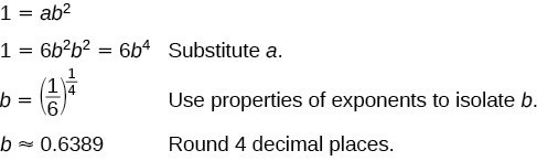
Use the value of b in the first equation to solve for the value of a:
![]()
Thus, the equation is [latex]f\left(x\right)=2.4492{\left(0.6389\right)}^{x}\\[/latex].
We can graph our model to check our work. Notice that the graph below passes through the initial points given in the problem, [latex]\left(-2,\text{ 6}\right)\\[/latex] and [latex]\left(2,\text{ 1}\right)\\[/latex]. The graph is an example of an exponential decay function.
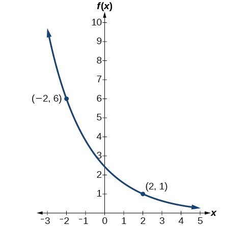
Figure 4. The graph of [latex]f\left(x\right)=2.4492{\left(0.6389\right)}^{x}\\[/latex] models exponential decay.
Given the two points [latex]\left(1,3\right)\\[/latex] and [latex]\left(2,4.5\right)\\[/latex], find the equation of the exponential function that passes through these two points.
Do two points always determine a unique exponential function?
Yes, provided the two points are either both above the x-axis or both below the x-axis and have different x-coordinates. But keep in mind that we also need to know that the graph is, in fact, an exponential function. Not every graph that looks exponential really is exponential. We need to know the graph is based on a model that shows the same percent growth with each unit increase in x, which in many real world cases involves time.
Find an equation for the exponential function graphed in Figure 5.
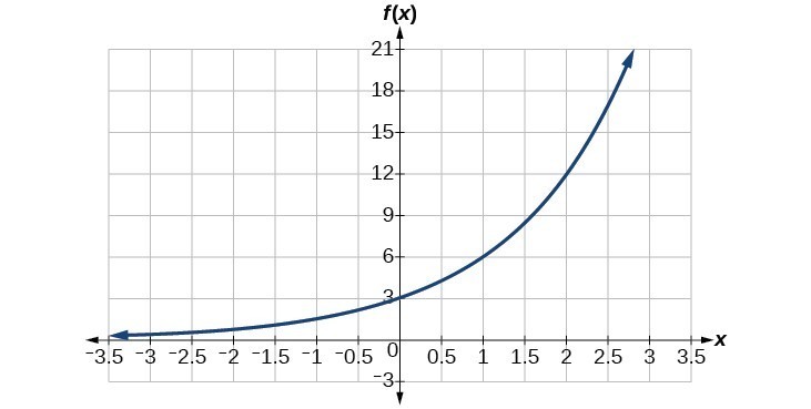
Figure 5
We can choose the y-intercept of the graph, [latex]\left(0,3\right)\\[/latex], as our first point. This gives us the initial value, [latex]a=3\\[/latex]. Next, choose a point on the curve some distance away from [latex]\left(0,3\right)\\[/latex] that has integer coordinates. One such point is [latex]\left(2,12\right)\\[/latex].
Because we restrict ourselves to positive values of b, we will use b = 2. Substitute a and b into the standard form to yield the equation [latex]f\left(x\right)=3{\left(2\right)}^{x}\\[/latex].
Use a graphing calculator to find the exponential equation that includes the points [latex]\left(2,24.8\right)\\[/latex] and [latex]\left(5,198.4\right)\\[/latex].
Follow the guidelines above. First press [STAT], [EDIT], [1: Edit…], and clear the lists L1 and L2. Next, in the L1 column, enter the x-coordinates, 2 and 5. Do the same in the L2 column for the y-coordinates, 24.8 and 198.4.
Now press [STAT], [CALC], [0: ExpReg] and press [ENTER]. The values a = 6.2 and b = 2 will be displayed. The exponential equation is [latex]y=6.2\cdot {2}^{x}\\[/latex].
Use a graphing calculator to find the exponential equation that includes the points (3, 75.98) and (6, 481.07).
Savings instruments in which earnings are continually reinvested, such as mutual funds and retirement accounts, use compound interest. The term compounding refers to interest earned not only on the original value, but on the accumulated value of the account.
The annual percentage rate (APR) of an account, also called the nominal rate, is the yearly interest rate earned by an investment account. The term nominal is used when the compounding occurs a number of times other than once per year. In fact, when interest is compounded more than once a year, the effective interest rate ends up being greater than the nominal rate! This is a powerful tool for investing.
We can calculate the compound interest using the compound interest formula, which is an exponential function of the variables time t, principal P, APR r, and number of compounding periods in a year n:
For example, observe the table below, which shows the result of investing $1,000 at 10% for one year. Notice how the value of the account increases as the compounding frequency increases.
| Frequency | Value after 1 year |
|---|---|
| Annually | $1100 |
| Semiannually | $1102.50 |
| Quarterly | $1103.81 |
| Monthly | $1104.71 |
| Daily | $1105.16 |
Compound interest can be calculated using the formula
where
If we invest $3,000 in an investment account paying 3% interest compounded quarterly, how much will the account be worth in 10 years?
Because we are starting with $3,000, P = 3000. Our interest rate is 3%, so r = 0.03. Because we are compounding quarterly, we are compounding 4 times per year, so n = 4. We want to know the value of the account in 10 years, so we are looking for A(10), the value when t = 10.
The account will be worth about $4,045.05 in 10 years.
An initial investment of $100,000 at 12% interest is compounded weekly (use 52 weeks in a year). What will the investment be worth in 30 years?
A 529 Plan is a college-savings plan that allows relatives to invest money to pay for a child’s future college tuition; the account grows tax-free. Lily wants to set up a 529 account for her new granddaughter and wants the account to grow to $40,000 over 18 years. She believes the account will earn 6% compounded semi-annually (twice a year). To the nearest dollar, how much will Lily need to invest in the account now?
The nominal interest rate is 6%, so r = 0.06. Interest is compounded twice a year, so k = 2.
We want to find the initial investment, P, needed so that the value of the account will be worth $40,000 in 18 years. Substitute the given values into the compound interest formula, and solve for P.
Lily will need to invest $13,801 to have $40,000 in 18 years.
Refer to Example 8. To the nearest dollar, how much would Lily need to invest if the account is compounded quarterly?
As we saw earlier, the amount earned on an account increases as the compounding frequency increases. The table below shows that the increase from annual to semi-annual compounding is larger than the increase from monthly to daily compounding. This might lead us to ask whether this pattern will continue.
Examine the value of $1 invested at 100% interest for 1 year, compounded at various frequencies.
| Frequency | [latex]A\left(t\right)={\left(1+\frac{1}{n}\right)}^{n}\\[/latex] | Value |
|---|---|---|
| Annually | [latex]{\left(1+\frac{1}{1}\right)}^{1}\\[/latex] | $2 |
| Semiannually | [latex]{\left(1+\frac{1}{2}\right)}^{2}\\[/latex] | $2.25 |
| Quarterly | [latex]{\left(1+\frac{1}{4}\right)}^{4}\\[/latex] | $2.441406 |
| Monthly | [latex]{\left(1+\frac{1}{12}\right)}^{12}\\[/latex] | $2.613035 |
| Daily | [latex]{\left(1+\frac{1}{365}\right)}^{365}\\[/latex] | $2.714567 |
| Hourly | [latex]{\left(1+\frac{1}{\text{8766}}\right)}^{\text{8766}}\\[/latex] | $2.718127 |
| Once per minute | [latex]{\left(1+\frac{1}{\text{525960}}\right)}^{\text{525960}}\\[/latex] | $2.718279 |
| Once per second | [latex]{\left(1+\frac{1}{31557600}\right)}^{31557600}\\[/latex] | $2.718282 |
These values appear to be approaching a limit as n increases without bound. In fact, as n gets larger and larger, the expression [latex]{\left(1+\frac{1}{n}\right)}^{n}\\[/latex] approaches a number used so frequently in mathematics that it has its own name: the letter [latex]e[/latex]. This value is an irrational number, which means that its decimal expansion goes on forever without repeating. Its approximation to six decimal places is shown below.
The letter e represents the irrational number
The letter e is used as a base for many real-world exponential models. To work with base e, we use the approximation, [latex]e\approx 2.718282\\[/latex]. The constant was named by the Swiss mathematician Leonhard Euler (1707–1783) who first investigated and discovered many of its properties.
Calculate [latex]{e}^{3.14}\\[/latex]. Round to five decimal places.
On a calculator, press the button labeled [latex]\left[{e}^{x}\right]\\[/latex]. The window shows [e^(]. Type 3.14 and then close parenthesis, (]). Press [ENTER]. Rounding to 5 decimal places, [latex]{e}^{3.14}\approx 23.10387\\[/latex]. Caution: Many scientific calculators have an “Exp” button, which is used to enter numbers in scientific notation. It is not used to find powers of e.
Use a calculator to find [latex]{e}^{-0.5}\\[/latex]. Round to five decimal places.
So far we have worked with rational bases for exponential functions. For most real-world phenomena, however, e is used as the base for exponential functions. Exponential models that use e as the base are called continuous growth or decay models. We see these models in finance, computer science, and most of the sciences, such as physics, toxicology, and fluid dynamics.
For all real numbers t, and all positive numbers a and r, continuous growth or decay is represented by the formula
where
If r > 0, then the formula represents continuous growth. If r < 0, then the formula represents continuous decay.
For business applications, the continuous growth formula is called the continuous compounding formula and takes the form
where
A person invested $1,000 in an account earning a nominal 10% per year compounded continuously. How much was in the account at the end of one year?
Since the account is growing in value, this is a continuous compounding problem with growth rate r = 0.10. The initial investment was $1,000, so P = 1000. We use the continuous compounding formula to find the value after t = 1 year:
The account is worth $1,105.17 after one year.
A person invests $100,000 at a nominal 12% interest per year compounded continuously. What will be the value of the investment in 30 years?
Radon-222 decays at a continuous rate of 17.3% per day. How much will 100 mg of Radon-222 decay to in 3 days?
Since the substance is decaying, the rate, 17.3%, is negative. So, r = –0.173. The initial amount of radon-222 was 100 mg, so a = 100. We use the continuous decay formula to find the value after t = 3 days:
So 59.5115 mg of radon-222 will remain.
| definition of the exponential function | [latex]f\left(x\right)={b}^{x}\text{, where }b>0, b\ne 1\\[/latex] |
| definition of exponential growth | [latex]f\left(x\right)=a{b}^{x},\text{ where }a>0,b>0,b\ne 1\\[/latex] |
| compound interest formula | [latex]\begin{cases}A\left(t\right)=P{\left(1+\frac{r}{n}\right)}^{nt} ,\text{ where}\hfill \\ A\left(t\right)\text{ is the account value at time }t\hfill \\ t\text{ is the number of years}\hfill \\ P\text{ is the initial investment, often called the principal}\hfill \\ r\text{ is the annual percentage rate (APR), or nominal rate}\hfill \\ n\text{ is the number of compounding periods in one year}\hfill \end{cases}\\[/latex] |
| continuous growth formula | [latex]A\left(t\right)=a{e}^{rt},\text{ where}\\[/latex]t is the number of unit time periods of growth a is the starting amount (in the continuous compounding formula a is replaced with P, the principal) e is the mathematical constant, [latex] e\approx 2.718282\\[/latex] |
1. Explain why the values of an increasing exponential function will eventually overtake the values of an increasing linear function.
2. Given a formula for an exponential function, is it possible to determine whether the function grows or decays exponentially just by looking at the formula? Explain.
3. The Oxford Dictionary defines the word nominal as a value that is “stated or expressed but not necessarily corresponding exactly to the real value.” (Oxford Dictionary. http://oxforddictionaries.com/us/definition/american_english/nomina.) Develop a reasonable argument for why the term nominal rate is used to describe the annual percentage rate of an investment account that compounds interest.
For the following exercises, identify whether the statement represents an exponential function. Explain.
4. The average annual population increase of a pack of wolves is 25.
5. A population of bacteria decreases by a factor of [latex]\frac{1}{8}\\[/latex] every 24 hours.
6. The value of a coin collection has increased by 3.25% annually over the last 20 years.
7. For each training session, a personal trainer charges his clients $5 less than the previous training session.
8. The height of a projectile at time t is represented by the function [latex]h\left(t\right)=-4.9{t}^{2}+18t+40\\[/latex].
For the following exercises, consider this scenario: For each year t, the population of a forest of trees is represented by the function [latex]A\left(t\right)=115{\left(1.025\right)}^{t}\\[/latex]. In a neighboring forest, the population of the same type of tree is represented by the function [latex]B\left(t\right)=82{\left(1.029\right)}^{t}\\[/latex]. (Round answers to the nearest whole number.)
9. Which forest’s population is growing at a faster rate?
10. Which forest had a greater number of trees initially? By how many?
11. Assuming the population growth models continue to represent the growth of the forests, which forest will have a greater number of trees after 20 years? By how many?
12. Assuming the population growth models continue to represent the growth of the forests, which forest will have a greater number of trees after 100 years? By how many?
13. Discuss the above results from the previous four exercises. Assuming the population growth models continue to represent the growth of the forests, which forest will have the greater number of trees in the long run? Why? What are some factors that might influence the long-term validity of the exponential growth model?
For the following exercises, determine whether the equation represents exponential growth, exponential decay, or neither. Explain.
14. [latex]y=300{\left(1-t\right)}^{5}\\[/latex]
15. [latex]y=220{\left(1.06\right)}^{x}\\[/latex]
16. [latex]y=16.5{\left(1.025\right)}^{\frac{1}{x}}\\[/latex]
17. [latex]y=11,701{\left(0.97\right)}^{t}\\[/latex]
For the following exercises, find the formula for an exponential function that passes through the two points given.
18. [latex]\left(0,6\right)\\[/latex] and [latex]\left(3,750\right)\\[/latex]
19. [latex]\left(0,2000\right)\\[/latex] and [latex]\left(2,20\right)\\[/latex]
20. [latex]\left(-1,\frac{3}{2}\right)\\[/latex] and [latex]\left(3,24\right)\\[/latex]
21. [latex]\left(-2,6\right)\\[/latex] and [latex]\left(3,1\right)\\[/latex]
22. [latex]\left(3,1\right)\\[/latex] and [latex]\left(5,4\right)\\[/latex]
For the following exercises, determine whether the table could represent a function that is linear, exponential, or neither. If it appears to be exponential, find a function that passes through the points.
23.
| x | 1 | 2 | 3 | 4 |
| f(x) | 70 | 40 | 10 | -20 |
24.
| x | 1 | 2 | 3 | 4 |
| h(x) | 70 | 49 | 34.3 | 24.01 |
25.
| x | 1 | 2 | 3 | 4 |
| m(x) | 80 | 61 | 42.9 | 25.61 |
26.
| x | 1 | 2 | 3 | 4 |
| f(x) | 10 | 20 | 40 | 80 |
27.
| x | 1 | 2 | 3 | 4 |
| g(x) | -3.25 | 2 | 7.25 | 12.5 |
For the following exercises, use the compound interest formula, [latex]A\left(t\right)=P{\left(1+\frac{r}{n}\right)}^{nt}\\[/latex].
28. After a certain number of years, the value of an investment account is represented by the equation [latex]10,250{\left(1+\frac{0.04}{12}\right)}^{120}\\[/latex]. What is the value of the account?
29. What was the initial deposit made to the account in the previous exercise?
30. How many years had the account from the previous exercise been accumulating interest?
31. An account is opened with an initial deposit of $6,500 and earns 3.6% interest compounded semi-annually. What will the account be worth in 20 years?
32. How much more would the account in the previous exercise have been worth if the interest were compounding weekly?
33. Solve the compound interest formula for the principal, P.
34. Use the formula found in the previous exercise to calculate the initial deposit of an account that is worth $14,472.74 after earning 5.5% interest compounded monthly for 5 years. (Round to the nearest dollar.)
35. How much more would the account in the previous two exercises be worth if it were earning interest for 5 more years?
36. Use properties of rational exponents to solve the compound interest formula for the interest rate, r.
37. Use the formula found in the previous exercise to calculate the interest rate for an account that was compounded semi-annually, had an initial deposit of $9,000 and was worth $13,373.53 after 10 years.
38. Use the formula found in the previous exercise to calculate the interest rate for an account that was compounded monthly, had an initial deposit of $5,500, and was worth $38,455 after 30 years.
For the following exercises, determine whether the equation represents continuous growth, continuous decay, or neither. Explain.
39. [latex]y=3742{\left(e\right)}^{0.75t}\\[/latex]
40. [latex]y=150{\left(e\right)}^{\frac{3.25}{t}}\\[/latex]
41. [latex]y=2.25{\left(e\right)}^{-2t}\\[/latex]
42. Suppose an investment account is opened with an initial deposit of $12,000 earning 7.2% interest compounded continuously. How much will the account be worth after 30 years?
43. How much less would the account from Exercise 42 be worth after 30 years if it were compounded monthly instead?
For the following exercises, evaluate each function. Round answers to four decimal places, if necessary.
44. [latex]f\left(x\right)=2{\left(5\right)}^{x}\\[/latex], for [latex]f\left(-3\right)\\[/latex]
45. [latex]f\left(x\right)=-{4}^{2x+3}\\[/latex], for [latex]f\left(-1\right)\\[/latex]
46. [latex]f\left(x\right)={e}^{x}\\[/latex], for [latex]f\left(3\right)\\[/latex]
47. [latex]f\left(x\right)=-2{e}^{x - 1}\\[/latex], for [latex]f\left(-1\right)\\[/latex]
48. [latex]f\left(x\right)=2.7{\left(4\right)}^{-x+1}+1.5\\[/latex], for [latex]f\left(-2\right)\\[/latex]
49. [latex]f\left(x\right)=1.2{e}^{2x}-0.3\\[/latex], for [latex]f\left(3\right)\\[/latex]
50. [latex]f\left(x\right)=-\frac{3}{2}{\left(3\right)}^{-x}+\frac{3}{2}\\[/latex], for [latex]f\left(2\right)\\[/latex]
For the following exercises, use a graphing calculator to find the equation of an exponential function given the points on the curve.
51. [latex]\left(0,3\right)\\[/latex] and [latex]\left(3,375\right)\\[/latex]
52. [latex]\left(3,222.62\right)\\[/latex] and [latex]\left(10,77.456\right)\\[/latex]
53. [latex]\left(20,29.495\right)\\[/latex] and [latex]\left(150,730.89\right)\\[/latex]
54. [latex]\left(5,2.909\right)\\[/latex] and [latex]\left(13,0.005\right)\\[/latex]
55. [latex]\left(11,310.035\right)\\[/latex] and [latex]\left(25,356.3652\right)\\[/latex]
56. The annual percentage yield (APY) of an investment account is a representation of the actual interest rate earned on a compounding account. It is based on a compounding period of one year. Show that the APY of an account that compounds monthly can be found with the formula [latex]\text{APY}={\left(1+\frac{r}{12}\right)}^{12}-1\\[/latex].
57. Repeat the previous exercise to find the formula for the APY of an account that compounds daily. Use the results from this and the previous exercise to develop a function [latex]I\left(n\right)\\[/latex] for the APY of any account that compounds n times per year.
58. Recall that an exponential function is any equation written in the form [latex]f\left(x\right)=a\cdot {b}^{x}\\[/latex] such that a and b are positive numbers and [latex]b\ne 1\\[/latex]. Any positive number b can be written as [latex] b={e}^{n}\\[/latex] for some value of n. Use this fact to rewrite the formula for an exponential function that uses the number e as a base.
59. In an exponential decay function, the base of the exponent is a value between 0 and 1. Thus, for some number [latex]b>1\\[/latex], the exponential decay function can be written as [latex]f\left(x\right)=a\cdot {\left(\frac{1}{b}\right)}^{x}\\[/latex]. Use this formula, along with the fact that [latex]b={e}^{n}\\[/latex], to show that an exponential decay function takes the form [latex]f\left(x\right)=a{\left(e\right)}^{-nx}\\[/latex] for some positive number n.
60. The formula for the amount A in an investment account with a nominal interest rate r at any time t is given by [latex]A\left(t\right)=a{\left(e\right)}^{rt}\\[/latex], where a is the amount of principal initially deposited into an account that compounds continuously. Prove that the percentage of interest earned to principal at any time t can be calculated with the formula [latex]I\left(t\right)={e}^{rt}-1\\[/latex].
61. The fox population in a certain region has an annual growth rate of 9% per year. In the year 2012, there were 23,900 fox counted in the area. What is the fox population predicted to be in the year 2020?
62. A scientist begins with 100 milligrams of a radioactive substance that decays exponentially. After 35 hours, 50mg of the substance remains. How many milligrams will remain after 54 hours?
63. In the year 1985, a house was valued at $110,000. By the year 2005, the value had appreciated to $145,000. What was the annual growth rate between 1985 and 2005? Assume that the value continued to grow by the same percentage. What was the value of the house in the year 2010?
64. A car was valued at $38,000 in the year 2007. By 2013, the value had depreciated to $11,000 If the car’s value continues to drop by the same percentage, what will it be worth by 2017?
65. Jamal wants to save $54,000 for a down payment on a home. How much will he need to invest in an account with 8.2% APR, compounding daily, in order to reach his goal in 5 years?
66. Kyoko has $10,000 that she wants to invest. Her bank has several investment accounts to choose from, all compounding daily. Her goal is to have $15,000 by the time she finishes graduate school in 6 years. To the nearest hundredth of a percent, what should her minimum annual interest rate be in order to reach her goal? (Hint: solve the compound interest formula for the interest rate.)
67. Alyssa opened a retirement account with 7.25% APR in the year 2000. Her initial deposit was $13,500. How much will the account be worth in 2025 if interest compounds monthly? How much more would she make if interest compounded continuously?
68. An investment account with an annual interest rate of 7% was opened with an initial deposit of $4,000 Compare the values of the account after 9 years when the interest is compounded annually, quarterly, monthly, and continuously.
1. 5.5556
2. About 1.548 billion people; by the year 2031, India’s population will exceed China’s by about 0.001 billion, or 1 million people.
3. [latex]\left(0,129\right)\\[/latex] and [latex]\left(2,236\right);N\left(t\right)=129{\left(\text{1}\text{.3526}\right)}^{t}\\[/latex]
4. [latex]f\left(x\right)=2{\left(1.5\right)}^{x}\\[/latex]
5. [latex]f\left(x\right)=\sqrt{2}{\left(\sqrt{2}\right)}^{x}\\[/latex]. Answers may vary due to round-off error. The answer should be very close to [latex]1.4142{\left(1.4142\right)}^{x}\\[/latex].
6. [latex]y\approx 12\cdot {1.85}^{x}\\[/latex]
7. about $3,644,675.88
8. $13,693
9. [latex]{e}^{-0.5}\approx 0.60653\\[/latex]
10. $3,659,823.44
11. 3.77E-26 (This is calculator notation for the number written as [latex]3.77\times {10}^{-26}\\[/latex] in scientific notation. While the output of an exponential function is never zero, this number is so close to zero that for all practical purposes we can accept zero as the answer.)
1. Linear functions have a constant rate of change. Exponential functions increase based on a percent of the original.
3. When interest is compounded, the percentage of interest earned to principal ends up being greater than the annual percentage rate for the investment account. Thus, the annual percentage rate does not necessarily correspond to the real interest earned, which is the very definition of nominal.
5. exponential; the population decreases by a proportional rate.
7. not exponential; the charge decreases by a constant amount each visit, so the statement represents a linear function.
9. The forest represented by the function [latex]B\left(t\right)=82{\left(1.029\right)}^{t}\\[/latex].
11. After t = 20 years, forest A will have 43 more trees than forest B.
13. Answers will vary. Sample response: For a number of years, the population of forest A will increasingly exceed forest B, but because forest B actually grows at a faster rate, the population will eventually become larger than forest A and will remain that way as long as the population growth models hold. Some factors that might influence the long-term validity of the exponential growth model are drought, an epidemic that culls the population, and other environmental and biological factors.
15. exponential growth; The growth factor, 1.06, is greater than 1.
17. exponential decay; The decay factor, 0.97, is between 0 and 1.
19. [latex]f\left(x\right)=2000{\left(0.1\right)}^{x}\\[/latex]
21. [latex]f\left(x\right)={\left(\frac{1}{6}\right)}^{-\frac{3}{5}}{\left(\frac{1}{6}\right)}^{\frac{x}{5}}\approx 2.93{\left(0.699\right)}^{x}\\[/latex]
23. Linear
25. Neither
27. Linear
29. $10,250
31. $13,268.58
33. [latex]P=A\left(t\right)\cdot {\left(1+\frac{r}{n}\right)}^{-nt}\\[/latex]
35. $4,572.56
37. 4%
39. continuous growth; the growth rate is greater than 0.
41. continuous decay; the growth rate is less than 0.
43. $669.42
45. [latex]f\left(-1\right)=-4\\[/latex]
47. [latex]f\left(-1\right)\approx -0.2707\\[/latex]
49. [latex]f\left(3\right)\approx 483.8146\\[/latex]
51. [latex]y=3\cdot {5}^{x}\\[/latex]
53. [latex]y\approx 18\cdot {1.025}^{x}\\[/latex]
55. [latex]y\approx 0.2\cdot {1.95}^{x}\\[/latex]
57. [latex]\text{APY}=\frac{A\left(t\right)-a}{a}=\frac{a{\left(1+\frac{r}{365}\right)}^{365\left(1\right)}-a}{a}=\frac{a\left[{\left(1+\frac{r}{365}\right)}^{365}-1\right]}{a}={\left(1+\frac{r}{365}\right)}^{365}-1\\[/latex]; [latex]I\left(n\right)={\left(1+\frac{r}{n}\right)}^{n}-1\\[/latex]
59. Let f be the exponential decay function [latex]f\left(x\right)=a\cdot {\left(\frac{1}{b}\right)}^{x}\\[/latex] such that [latex]b>1\\[/latex]. Then for some number [latex]n>0\\[/latex], [latex]f\left(x\right)=a\cdot {\left(\frac{1}{b}\right)}^{x}=a{\left({b}^{-1}\right)}^{x}=a{\left({\left({e}^{n}\right)}^{-1}\right)}^{x}=a{\left({e}^{-n}\right)}^{x}=a{\left(e\right)}^{-nx}\\[/latex].
61. 47,622 fox
63. 1.39%; $155,368.09
65. $35,838.76
67. $82,247.78; $449.75
By the end of this lesson, you will be able to:
As we discussed in the previous section, exponential functions are used for many real-world applications such as finance, forensics, computer science, and most of the life sciences. Working with an equation that describes a real-world situation gives us a method for making predictions. Most of the time, however, the equation itself is not enough. We learn a lot about things by seeing their pictorial representations, and that is exactly why graphing exponential equations is a powerful tool. It gives us another layer of insight for predicting future events.
Before we begin graphing, it is helpful to review the behavior of exponential growth. Recall the table of values for a function of the form [latex]f\left(x\right)={b}^{x}\\[/latex] whose base is greater than one. We’ll use the function [latex]f\left(x\right)={2}^{x}\\[/latex]. Observe how the output values in the table below change as the input increases by 1.
| x | –3 | –2 | –1 | 0 | 1 | 2 | 3 |
| [latex]f\left(x\right)={2}^{x}\\[/latex] | [latex]\frac{1}{8}\\[/latex] | [latex]\frac{1}{4}\\[/latex] | [latex]\frac{1}{2}\\[/latex] | 1 | 2 | 4 | 8 |
Each output value is the product of the previous output and the base, 2. We call the base 2 the constant ratio. In fact, for any exponential function with the form [latex]f\left(x\right)=a{b}^{x}\\[/latex], b is the constant ratio of the function. This means that as the input increases by 1, the output value will be the product of the base and the previous output, regardless of the value of a.
Notice from the table that
Figure 1 shows the exponential growth function [latex]f\left(x\right)={2}^{x}\\[/latex].
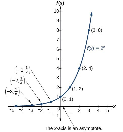
Figure 1. Notice that the graph gets close to the x-axis, but never touches it.
The domain of [latex]f\left(x\right)={2}^{x}\\[/latex] is all real numbers, the range is [latex]\left(0,\infty \right)\\[/latex], and the horizontal asymptote is [latex]y=0\\[/latex].
To get a sense of the behavior of exponential decay, we can create a table of values for a function of the form [latex]f\left(x\right)={b}^{x}\\[/latex] whose base is between zero and one. We’ll use the function [latex]g\left(x\right)={\left(\frac{1}{2}\right)}^{x}\\[/latex]. Observe how the output values in the table below change as the input increases by 1.
| x | –3 | –2 | –1 | 0 | 1 | 2 | 3 |
| [latex]g\left(x\right)=\left(\frac{1}{2}\right)^{x}\\[/latex] | 8 | 4 | 2 | 1 | [latex]\frac{1}{2}\\[/latex] | [latex]\frac{1}{4}\\[/latex] | [latex]\frac{1}{8}\\[/latex] |
Again, because the input is increasing by 1, each output value is the product of the previous output and the base, or constant ratio [latex]\frac{1}{2}\\[/latex].
Notice from the table that
The graph shows the exponential decay function, [latex]g\left(x\right)={\left(\frac{1}{2}\right)}^{x}\\[/latex].
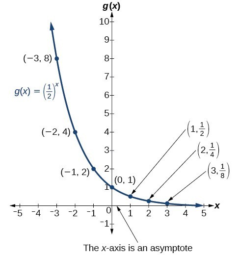
Figure 2. The domain of [latex]g\left(x\right)={\left(\frac{1}{2}\right)}^{x}\\[/latex] is all real numbers, the range is [latex]\left(0,\infty \right)\\[/latex], and the horizontal asymptote is [latex]y=0\\[/latex].
An exponential function with the form [latex]f\left(x\right)={b}^{x}\\[/latex], [latex]b>0\\[/latex], [latex]b\ne 1\\[/latex], has these characteristics:
Compare the graphs of exponential growth and decay functions.
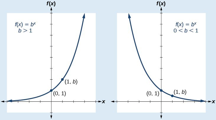
Figure 3
Sketch a graph of [latex]f\left(x\right)={0.25}^{x}\\[/latex]. State the domain, range, and asymptote.
Before graphing, identify the behavior and create a table of points for the graph.
| x | –3 | –2 | –1 | 0 | 1 | 2 | 3 |
| [latex]f\left(x\right)={0.25}^{x}\\[/latex] | 64 | 16 | 4 | 1 | 0.25 | 0.0625 | 0.015625 |
Draw a smooth curve connecting the points.
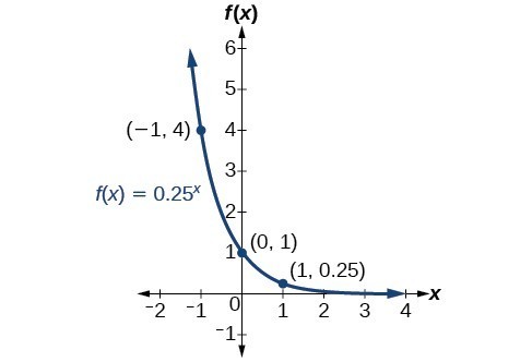
Figure 4. The domain is [latex]\left(-\infty ,\infty \right)\\[/latex]; the range is [latex]\left(0,\infty \right)\\[/latex]; the horizontal asymptote is [latex]y=0\\[/latex].
Sketch the graph of [latex]f\left(x\right)={4}^{x}\\[/latex]. State the domain, range, and asymptote.
Transformations of exponential graphs behave similarly to those of other functions. Just as with other parent functions, we can apply the four types of transformations—shifts, reflections, stretches, and compressions—to the parent function [latex]f\left(x\right)={b}^{x}\\[/latex] without loss of shape. For instance, just as the quadratic function maintains its parabolic shape when shifted, reflected, stretched, or compressed, the exponential function also maintains its general shape regardless of the transformations applied.
The first transformation occurs when we add a constant d to the parent function [latex]f\left(x\right)={b}^{x}\\[/latex], giving us a vertical shift d units in the same direction as the sign. For example, if we begin by graphing a parent function, [latex]f\left(x\right)={2}^{x}\\[/latex], we can then graph two vertical shifts alongside it, using [latex]d=3\\[/latex]: the upward shift, [latex]g\left(x\right)={2}^{x}+3\\[/latex] and the downward shift, [latex]h\left(x\right)={2}^{x}-3\\[/latex]. Both vertical shifts are shown in Figure 5.
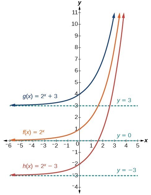
Figure 5
Observe the results of shifting [latex]f\left(x\right)={2}^{x}\\[/latex] vertically:
The next transformation occurs when we add a constant c to the input of the parent function [latex]f\left(x\right)={b}^{x}\\[/latex], giving us a horizontal shift c units in the opposite direction of the sign. For example, if we begin by graphing the parent function [latex]f\left(x\right)={2}^{x}\\[/latex], we can then graph two horizontal shifts alongside it, using [latex]c=3\\[/latex]: the shift left, [latex]g\left(x\right)={2}^{x+3}\\[/latex], and the shift right, [latex]h\left(x\right)={2}^{x - 3}\\[/latex]. Both horizontal shifts are shown in Figure 6.
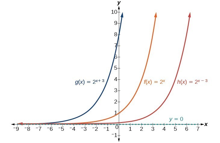
Figure 6
Observe the results of shifting [latex]f\left(x\right)={2}^{x}\\[/latex] horizontally:
For any constants c and d, the function [latex]f\left(x\right)={b}^{x+c}+d\\[/latex] shifts the parent function [latex]f\left(x\right)={b}^{x}\\[/latex]
Graph [latex]f\left(x\right)={2}^{x+1}-3\\[/latex]. State the domain, range, and asymptote.
We have an exponential equation of the form [latex]f\left(x\right)={b}^{x+c}+d\\[/latex], with [latex]b=2\\[/latex], [latex]c=1\\[/latex], and [latex]d=-3\\[/latex].
Draw the horizontal asymptote [latex]y=d\\[/latex], so draw [latex]y=-3\\[/latex].
Identify the shift as [latex]\left(-c,d\right)\\[/latex], so the shift is [latex]\left(-1,-3\right)\\[/latex].
Shift the graph of [latex]f\left(x\right)={b}^{x}\\[/latex] left 1 units and down 3 units.
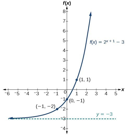
Figure 7. The domain is [latex]\left(-\infty ,\infty \right)\\[/latex]; the range is [latex]\left(-3,\infty \right)\\[/latex]; the horizontal asymptote is [latex]y=-3\\[/latex].
Graph [latex]f\left(x\right)={2}^{x - 1}+3\\[/latex]. State domain, range, and asymptote.
Solve [latex]42=1.2{\left(5\right)}^{x}+2.8\\[/latex] graphically. Round to the nearest thousandth.
Press [Y=] and enter [latex]1.2{\left(5\right)}^{x}+2.8\\[/latex] next to Y1=. Then enter 42 next to Y2=. For a window, use the values –3 to 3 for x and –5 to 55 for y. Press [GRAPH]. The graphs should intersect somewhere near x = 2.
For a better approximation, press [2ND] then [CALC]. Select [5: intersect] and press [ENTER] three times. The x-coordinate of the point of intersection is displayed as 2.1661943. (Your answer may be different if you use a different window or use a different value for Guess?) To the nearest thousandth, [latex]x\approx 2.166\\[/latex].
Solve [latex]4=7.85{\left(1.15\right)}^{x}-2.27\\[/latex] graphically. Round to the nearest thousandth.
While horizontal and vertical shifts involve adding constants to the input or to the function itself, a stretch or compression occurs when we multiply the parent function [latex]f\left(x\right)={b}^{x}\\[/latex] by a constant [latex]|a|>0\\[/latex]. For example, if we begin by graphing the parent function [latex]f\left(x\right)={2}^{x}\\[/latex], we can then graph the stretch, using [latex]a=3\\[/latex], to get [latex]g\left(x\right)=3{\left(2\right)}^{x}\\[/latex] as shown on the left in Figure 8, and the compression, using [latex]a=\frac{1}{3}\\[/latex], to get [latex]h\left(x\right)=\frac{1}{3}{\left(2\right)}^{x}\\[/latex] as shown on the right in Figure 8.
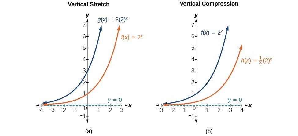
Figure 8. (a) [latex]g\left(x\right)=3{\left(2\right)}^{x}\\[/latex] stretches the graph of [latex]f\left(x\right)={2}^{x}\\[/latex] vertically by a factor of 3. (b) [latex]h\left(x\right)=\frac{1}{3}{\left(2\right)}^{x}\\[/latex] compresses the graph of [latex]f\left(x\right)={2}^{x}\\[/latex] vertically by a factor of [latex]\frac{1}{3}\\[/latex].
For any factor a > 0, the function [latex]f\left(x\right)=a{\left(b\right)}^{x}\\[/latex]
Sketch a graph of [latex]f\left(x\right)=4{\left(\frac{1}{2}\right)}^{x}\\[/latex]. State the domain, range, and asymptote.
Before graphing, identify the behavior and key points on the graph.
| x | –3 | –2 | –1 | 0 | 1 | 2 | 3 |
| [latex]f\left(x\right)=4\left(\frac{1}{2}\right)^{x}\\[/latex] | 32 | 16 | 8 | 4 | 2 | 1 | 0.5 |
Draw a smooth curve connecting the points.
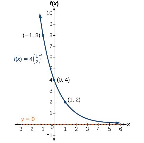
Figure 9. The domain is [latex]\left(-\infty ,\infty \right)\\[/latex]; the range is [latex]\left(0,\infty \right)\\[/latex]; the horizontal asymptote is y = 0.
Sketch the graph of [latex]f\left(x\right)=\frac{1}{2}{\left(4\right)}^{x}\\[/latex]. State the domain, range, and asymptote.
In addition to shifting, compressing, and stretching a graph, we can also reflect it about the x-axis or the y-axis. When we multiply the parent function [latex]f\left(x\right)={b}^{x}\\[/latex] by –1, we get a reflection about the x-axis. When we multiply the input by –1, we get a reflection about the y-axis. For example, if we begin by graphing the parent function [latex]f\left(x\right)={2}^{x}\\[/latex], we can then graph the two reflections alongside it. The reflection about the x-axis, [latex]g\left(x\right)={-2}^{x}\\[/latex], is shown on the left side, and the reflection about the y-axis [latex]h\left(x\right)={2}^{-x}\\[/latex], is shown on the right side.
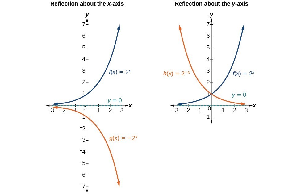
The function [latex]f\left(x\right)=-{b}^{x}\\[/latex]
The function [latex]f\left(x\right)={b}^{-x}\\[/latex]
Find and graph the equation for a function, [latex]g\left(x\right)\\[/latex], that reflects [latex]f\left(x\right)={\left(\frac{1}{4}\right)}^{x}\\[/latex] about the x-axis. State its domain, range, and asymptote.
Since we want to reflect the parent function [latex]f\left(x\right)={\left(\frac{1}{4}\right)}^{x}\\[/latex] about the x-axis, we multiply [latex]f\left(x\right)\\[/latex] by –1 to get, [latex]g\left(x\right)=-{\left(\frac{1}{4}\right)}^{x}\\[/latex]. Next we create a table of points.
| [latex]x[/latex] | –3 | –2 | –1 | 0 | 1 | 2 | 3 |
| [latex]g\left(x\right)=-\left(\frac{1}{4}\right)^{x}\\[/latex] | –64 | –16 | –4 | –1 | –0.25 | –0.0625 | –0.0156 |
Plot the y-intercept, [latex]\left(0,-1\right)\\[/latex], along with two other points. We can use [latex]\left(-1,-4\right)\\[/latex] and [latex]\left(1,-0.25\right)\\[/latex].
Draw a smooth curve connecting the points:
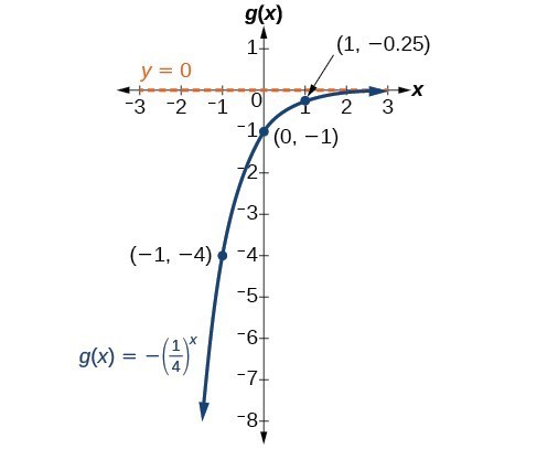
Figure 11. The domain is [latex]\left(-\infty ,\infty \right)\\[/latex]; the range is [latex]\left(-\infty ,0\right)\\[/latex]; the horizontal asymptote is [latex]y=0\\[/latex].
Find and graph the equation for a function, [latex]g\left(x\right)\\[/latex], that reflects [latex]f\left(x\right)={1.25}^{x}\\[/latex] about the y-axis. State its domain, range, and asymptote.
Now that we have worked with each type of translation for the exponential function, we can summarize them to arrive at the general equation for translating exponential functions.
| Translations of the Parent Function [latex]f\left(x\right)={b}^{x}\\[/latex] | |
|---|---|
| Translation | Form |
Shift
| [latex]f\left(x\right)={b}^{x+c}+d\\[/latex] |
Stretch and Compress
| [latex]f\left(x\right)=a{b}^{x}\\[/latex] |
| Reflect about the x-axis | [latex]f\left(x\right)=-{b}^{x}\\[/latex] |
| Reflect about the y-axis | [latex]f\left(x\right)={b}^{-x}={\left(\frac{1}{b}\right)}^{x}\\[/latex] |
| General equation for all translations | [latex]f\left(x\right)=a{b}^{x+c}+d\\[/latex] |
A translation of an exponential function has the form
Where the parent function, [latex]y={b}^{x}\\[/latex], [latex]b>1\\[/latex], is
Note the order of the shifts, transformations, and reflections follow the order of operations.
Write the equation for the function described below. Give the horizontal asymptote, the domain, and the range.
We want to find an equation of the general form [latex] f\left(x\right)=a{b}^{x+c}+d\\[/latex]. We use the description provided to find a, b, c, and d.
Substituting in the general form we get,
The domain is [latex]\left(-\infty ,\infty \right)\\[/latex]; the range is [latex]\left(4,\infty \right)\\[/latex]; the horizontal asymptote is [latex]y=4\\[/latex].
Write the equation for function described below. Give the horizontal asymptote, the domain, and the range.
| General Form for the Translation of the Parent Function [latex]\text{ }f\left(x\right)={b}^{x}\\[/latex] | [latex]f\left(x\right)=a{b}^{x+c}+d\\[/latex] |
1. What role does the horizontal asymptote of an exponential function play in telling us about the end behavior of the graph?
2. What is the advantage of knowing how to recognize transformations of the graph of a parent function algebraically?
3. The graph of [latex]f\left(x\right)={3}^{x}\\[/latex] is reflected about the y-axis and stretched vertically by a factor of 4. What is the equation of the new function, [latex]g\left(x\right)\\[/latex]? State its y-intercept, domain, and range.
4. The graph of [latex]f\left(x\right)={\left(\frac{1}{2}\right)}^{-x}\\[/latex] is reflected about the y-axis and compressed vertically by a factor of [latex]\frac{1}{5}\\[/latex]. What is the equation of the new function, [latex]g\left(x\right)\\[/latex]? State its y-intercept, domain, and range.
5. The graph of [latex]f\left(x\right)={10}^{x}\\[/latex] is reflected about the x-axis and shifted upward 7 units. What is the equation of the new function, [latex]g\left(x\right)\\[/latex]? State its y-intercept, domain, and range.
6. The graph of [latex]f\left(x\right)={\left(1.68\right)}^{x}\\[/latex] is shifted right 3 units, stretched vertically by a factor of 2, reflected about the x-axis, and then shifted downward 3 units. What is the equation of the new function, [latex]g\left(x\right)\\[/latex]? State its y-intercept (to the nearest thousandth), domain, and range.
7. The graph of [latex]f\left(x\right)=-\frac{1}{2}{\left(\frac{1}{4}\right)}^{x - 2}+4\\[/latex] is shifted left 2 units, stretched vertically by a factor of 4, reflected about the x-axis, and then shifted downward 4 units. What is the equation of the new function, [latex]g\left(x\right)\\[/latex]? State its y-intercept, domain, and range.
For the following exercises, graph the function and its reflection about the y-axis on the same axes, and give the y-intercept.
8. [latex]f\left(x\right)=3{\left(\frac{1}{2}\right)}^{x}\\[/latex]
9. [latex]g\left(x\right)=-2{\left(0.25\right)}^{x}\\[/latex]
10. [latex]h\left(x\right)=6{\left(1.75\right)}^{-x}\\[/latex]
For the following exercises, graph each set of functions on the same axes.
11. [latex]f\left(x\right)=3{\left(\frac{1}{4}\right)}^{x}\\[/latex], [latex]g\left(x\right)=3{\left(2\right)}^{x}\\[/latex], and [latex]h\left(x\right)=3{\left(4\right)}^{x}\\[/latex]
12. [latex]f\left(x\right)=\frac{1}{4}{\left(3\right)}^{x}\\[/latex], [latex]g\left(x\right)=2{\left(3\right)}^{x}\\[/latex], and [latex]h\left(x\right)=4{\left(3\right)}^{x}\\[/latex]
For the following exercises, match each function with one of the graphs pictured below.
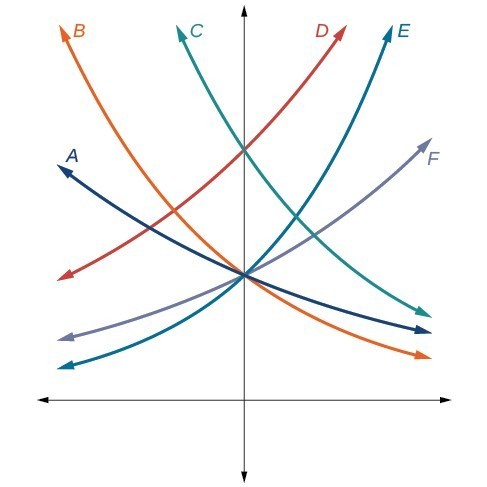
13. [latex]f\left(x\right)=2{\left(0.69\right)}^{x}\\[/latex]
14. [latex]f\left(x\right)=2{\left(1.28\right)}^{x}\\[/latex]
15. [latex]f\left(x\right)=2{\left(0.81\right)}^{x}\\[/latex]
16. [latex]f\left(x\right)=4{\left(1.28\right)}^{x}\\[/latex]
17. [latex]f\left(x\right)=2{\left(1.59\right)}^{x}\\[/latex]
18. [latex]f\left(x\right)=4{\left(0.69\right)}^{x}\\[/latex]
For the following exercises, use the graphs shown below. All have the form [latex]f\left(x\right)=a{b}^{x}\\[/latex].
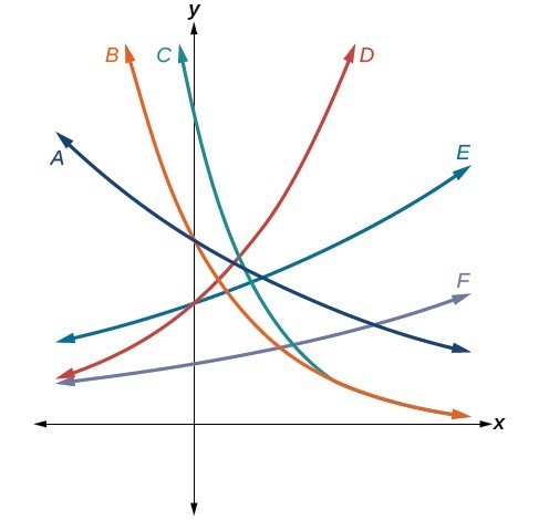
19. Which graph has the largest value for b?
20. Which graph has the smallest value for b?
21. Which graph has the largest value for a?
22. Which graph has the smallest value for a?
For the following exercises, graph the function and its reflection about the x-axis on the same axes.
23. [latex]f\left(x\right)=\frac{1}{2}{\left(4\right)}^{x}\\[/latex]
24. [latex]f\left(x\right)=3{\left(0.75\right)}^{x}-1\\[/latex]
25. [latex]f\left(x\right)=-4{\left(2\right)}^{x}+2\\[/latex]
For the following exercises, graph the transformation of [latex]f\left(x\right)={2}^{x}\\[/latex]. Give the horizontal asymptote, the domain, and the range.
26. [latex]f\left(x\right)={2}^{-x}\\[/latex]
27. [latex]h\left(x\right)={2}^{x}+3\\[/latex]
28. [latex]f\left(x\right)={2}^{x - 2}\\[/latex]
For the following exercises, describe the end behavior of the graphs of the functions.
29. [latex]f\left(x\right)=-5{\left(4\right)}^{x}-1\\[/latex]
30. [latex]f\left(x\right)=3{\left(\frac{1}{2}\right)}^{x}-2\\[/latex]
31. [latex]f\left(x\right)=3{\left(4\right)}^{-x}+2\\[/latex]
For the following exercises, start with the graph of [latex]f\left(x\right)={4}^{x}\\[/latex]. Then write a function that results from the given transformation.
32. Shift f(x) 4 units upward
33. Shift f(x) 3 units downward
34. Shift f(x) 2 units left
35. Shift f(x) 5 units right
36. Reflect f(x) about the x-axis
37. Reflect f(x) about the y-axis
For the following exercises, each graph is a transformation of [latex]y={2}^{x}\\[/latex]. Write an equation describing the transformation.
38.
39.
40.
For the following exercises, find an exponential equation for the graph.
41.
42.
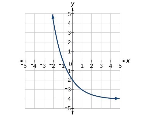
For the following exercises, evaluate the exponential functions for the indicated value of x.
43. [latex]g\left(x\right)=\frac{1}{3}{\left(7\right)}^{x - 2}\\[/latex] for [latex]g\left(6\right)\\[/latex].
44. [latex]f\left(x\right)=4{\left(2\right)}^{x - 1}-2\\[/latex] for [latex]f\left(5\right)\\[/latex].
45. [latex]h\left(x\right)=-\frac{1}{2}{\left(\frac{1}{2}\right)}^{x}+6\\[/latex] for [latex]h\left(-7\right)\\[/latex].
For the following exercises, use a graphing calculator to approximate the solutions of the equation. Round to the nearest thousandth. [latex]f\left(x\right)=a{b}^{x}+d\\[/latex].
46. [latex]-50=-{\left(\frac{1}{2}\right)}^{-x}\\[/latex]
47. [latex]116=\frac{1}{4}{\left(\frac{1}{8}\right)}^{x}\\[/latex]
48. [latex]12=2{\left(3\right)}^{x}+1\\[/latex]
49. [latex]5=3{\left(\frac{1}{2}\right)}^{x - 1}-2\\[/latex]
50. [latex]-30=-4{\left(2\right)}^{x+2}+2\\[/latex]
51. Explore and discuss the graphs of [latex]F\left(x\right)={\left(b\right)}^{x}\\[/latex] and [latex]G\left(x\right)={\left(\frac{1}{b}\right)}^{x}\\[/latex]. Then make a conjecture about the relationship between the graphs of the functions [latex]{b}^{x}\\[/latex] and [latex]{\left(\frac{1}{b}\right)}^{x}\\[/latex] for any real number [latex]b>0\\[/latex].
52. Prove the conjecture made in the previous exercise.
53. Explore and discuss the graphs of [latex]f\left(x\right)={4}^{x}\\[/latex], [latex]g\left(x\right)={4}^{x - 2}\\[/latex], and [latex]h\left(x\right)=\left(\frac{1}{16}\right){4}^{x}\\[/latex]. Then make a conjecture about the relationship between the graphs of the functions [latex]{b}^{x}\\[/latex] and [latex]\left(\frac{1}{{b}^{n}}\right){b}^{x}\\[/latex] for any real number n and real number [latex]b>0\\[/latex].
54. Prove the conjecture made in the previous exercise.
1. The domain is [latex]\left(-\infty ,\infty \right)\\[/latex]; the range is [latex]\left(0,\infty \right)\\[/latex]; the horizontal asymptote is [latex]y=0\\[/latex].

2. The domain is [latex]\left(-\infty ,\infty \right)\\[/latex]; the range is [latex]\left(3,\infty \right)\\[/latex]; the horizontal asymptote is y = 3.

3. [latex]x\approx -1.608\\[/latex]
4. The domain is [latex]\left(-\infty ,\infty \right)\\[/latex]; the range is [latex]\left(0,\infty \right)\\[/latex]; the horizontal asymptote is [latex]y=0\\[/latex].

5. The domain is [latex]\left(-\infty ,\infty \right)\\[/latex]; the range is [latex]\left(0,\infty \right)\\[/latex]; the horizontal asymptote is [latex]y=0\\[/latex].

6. [latex]f\left(x\right)=-\frac{1}{3}{e}^{x}-2\\[/latex]; the domain is [latex]\left(-\infty ,\infty \right)\\[/latex]; the range is [latex]\left(-\infty ,2\right)\\[/latex]; the horizontal asymptote is [latex]y=2\\[/latex].
1. An asymptote is a line that the graph of a function approaches, as x either increases or decreases without bound. The horizontal asymptote of an exponential function tells us the limit of the function’s values as the independent variable gets either extremely large or extremely small.
3. [latex]g\left(x\right)=4{\left(3\right)}^{-x}\\[/latex]; y-intercept: [latex]\left(0,4\right)\\[/latex]; Domain: all real numbers; Range: all real numbers greater than 0.
5. [latex]g\left(x\right)=-{10}^{x}+7\\[/latex]; y-intercept: [latex]\left(0,6\right)\\[/latex]; Domain: all real numbers; Range: all real numbers less than 7.
7. [latex]g\left(x\right)=2{\left(\frac{1}{4}\right)}^{x}\\[/latex]; y-intercept: [latex]\left(0,\text{ 2}\right)\\[/latex]; Domain: all real numbers; Range: all real numbers greater than 0.
9. y-intercept: [latex]\left(0,-2\right)\\[/latex]

11.

13. B
15. A
17. E
19. D
21. C
23.

25.

27. Horizontal asymptote: [latex]h\left(x\right)=3\\[/latex]; Domain: all real numbers; Range: all real numbers strictly greater than 3.

29. As [latex]x\to \infty \\[/latex] , [latex]f\left(x\right)\to -\infty\\ [/latex] ;
As [latex]x\to -\infty \\[/latex] , [latex]f\left(x\right)\to -1\\[/latex]
31. As [latex]x\to \infty\\ [/latex] , [latex]f\left(x\right)\to 2\\[/latex] ;
As [latex]x\to -\infty \\[/latex] , [latex]f\left(x\right)\to \infty \\[/latex]
33. [latex]f\left(x\right)={4}^{x}-3\\[/latex]
35. [latex]f\left(x\right)={4}^{x - 5}\\[/latex]
37. [latex]f\left(x\right)={4}^{-x}\\[/latex]
39. [latex]y=-{2}^{x}+3\\[/latex]
41. [latex]y=-2{\left(3\right)}^{x}+7\\[/latex]
43. [latex]g\left(6\right)=800+\frac{1}{3}\approx 800.3333\\[/latex]
45. [latex]h\left(-7\right)=-58\\[/latex]
47. [latex]x\approx -2.953\\[/latex]
49. [latex]x\approx -0.222\\[/latex]
51. The graph of [latex]G\left(x\right)={\left(\frac{1}{b}\right)}^{x}\\[/latex] is the reflection about the y-axis of the graph of [latex]F\left(x\right)={b}^{x}\\[/latex]; For any real number [latex]b>0\\[/latex] and function [latex]f\left(x\right)={b}^{x}\\[/latex], the graph of [latex]{\left(\frac{1}{b}\right)}^{x}\\[/latex] is the the reflection about the y-axis, [latex]F\left(-x\right)\\[/latex].
53. The graphs of [latex]g\left(x\right)\\[/latex] and [latex]h\left(x\right)\\[/latex] are the same and are a horizontal shift to the right of the graph of [latex]f\left(x\right)\\[/latex]; For any real number n, real number [latex]b>0\\[/latex], and function [latex]f\left(x\right)={b}^{x}\\[/latex], the graph of [latex]\left(\frac{1}{{b}^{n}}\right){b}^{x}\\[/latex] is the horizontal shift [latex]f\left(x-n\right)\\[/latex].
By the end of this lesson, you will be able to:

Figure 1. Devastation of March 11, 2011 earthquake in Honshu, Japan. (credit: Daniel Pierce)
In 2010, a major earthquake struck Haiti, destroying or damaging over 285,000 homes. (http://earthquake.usgs.gov/earthquakes/eqinthenews/2010/us2010rja6/#summary. Accessed 3/4/2013.) One year later, another, stronger earthquake devastated Honshu, Japan, destroying or damaging over 332,000 buildings, (http://earthquake.usgs.gov/earthquakes/eqinthenews/2011/usc0001xgp/#summary. Accessed 3/4/2013.) like those shown in the picture above. Even though both caused substantial damage, the earthquake in 2011 was 100 times stronger than the earthquake in Haiti. How do we know? The magnitudes of earthquakes are measured on a scale known as the Richter Scale. The Haitian earthquake registered a 7.0 on the Richter Scale (http://earthquake.usgs.gov/earthquakes/eqinthenews/2010/us2010rja6/. Accessed 3/4/2013.) whereas the Japanese earthquake registered a 9.0. (http://earthquake.usgs.gov/earthquakes/eqinthenews/2011/usc0001xgp/#details. Accessed 3/4/2013.)
The Richter Scale is a base-ten logarithmic scale. In other words, an earthquake of magnitude 8 is not twice as great as an earthquake of magnitude 4. It is [latex]{10}^{8 - 4}={10}^{4}=10,000\\[/latex] times as great! In this lesson, we will investigate the nature of the Richter Scale and the base-ten function upon which it depends.
In order to analyze the magnitude of earthquakes or compare the magnitudes of two different earthquakes, we need to be able to convert between logarithmic and exponential form. For example, suppose the amount of energy released from one earthquake were 500 times greater than the amount of energy released from another. We want to calculate the difference in magnitude. The equation that represents this problem is [latex]{10}^{x}=500\\[/latex], where x represents the difference in magnitudes on the Richter Scale. How would we solve for x?
We have not yet learned a method for solving exponential equations. None of the algebraic tools discussed so far is sufficient to solve [latex]{10}^{x}=500\\[/latex]. We know that [latex]{10}^{2}=100\\[/latex] and [latex]{10}^{3}=1000\\[/latex], so it is clear that x must be some value between 2 and 3, since [latex]y={10}^{x}\\[/latex] is increasing. We can examine a graph to better estimate the solution.
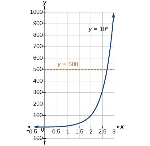
Figure 2
Estimating from a graph, however, is imprecise. To find an algebraic solution, we must introduce a new function. Observe that the graph above passes the horizontal line test. The exponential function [latex]y={b}^{x}\\[/latex] is one-to-one, so its inverse, [latex]x={b}^{y}\\[/latex] is also a function. As is the case with all inverse functions, we simply interchange x and y and solve for y to find the inverse function. To represent y as a function of x, we use a logarithmic function of the form [latex]y={\mathrm{log}}_{b}\left(x\right)\\[/latex]. The base b logarithm of a number is the exponent by which we must raise b to get that number.
We read a logarithmic expression as, “The logarithm with base b of x is equal to y,” or, simplified, “log base b of x is y.” We can also say, “b raised to the power of y is x,” because logs are exponents. For example, the base 2 logarithm of 32 is 5, because 5 is the exponent we must apply to 2 to get 32. Since [latex]{2}^{5}=32\\[/latex], we can write [latex]{\mathrm{log}}_{2}32=5\\[/latex]. We read this as “log base 2 of 32 is 5.”
We can express the relationship between logarithmic form and its corresponding exponential form as follows:
Note that the base b is always positive.

Because logarithm is a function, it is most correctly written as [latex]{\mathrm{log}}_{b}\left(x\right)\\[/latex], using parentheses to denote function evaluation, just as we would with [latex]f\left(x\right)\\[/latex]. However, when the input is a single variable or number, it is common to see the parentheses dropped and the expression written without parentheses, as [latex]{\mathrm{log}}_{b}x\\[/latex]. Note that many calculators require parentheses around the x.
We can illustrate the notation of logarithms as follows:

Notice that, comparing the logarithm function and the exponential function, the input and the output are switched. This means [latex]y={\mathrm{log}}_{b}\left(x\right)[/latex] and [latex]y={b}^{x}\\[/latex] are inverse functions.
A logarithm base b of a positive number x satisfies the following definition.
For [latex]x>0,b>0,b\ne 1\\[/latex],
where,
Also, since the logarithmic and exponential functions switch the x and y values, the domain and range of the exponential function are interchanged for the logarithmic function. Therefore,
Can we take the logarithm of a negative number?
No. Because the base of an exponential function is always positive, no power of that base can ever be negative. We can never take the logarithm of a negative number. Also, we cannot take the logarithm of zero. Calculators may output a log of a negative number when in complex mode, but the log of a negative number is not a real number.
Write the following logarithmic equations in exponential form.
First, identify the values of b, y, and x. Then, write the equation in the form [latex]{b}^{y}=x\\[/latex].
Here, [latex]b=6,y=\frac{1}{2},\text{and } x=\sqrt{6}\\[/latex]. Therefore, the equation [latex]{\mathrm{log}}_{6}\left(\sqrt{6}\right)=\frac{1}{2}\\[/latex] is equivalent to [latex]{6}^{\frac{1}{2}}=\sqrt{6}\\[/latex].
Here, b = 3, y = 2, and x = 9. Therefore, the equation [latex]{\mathrm{log}}_{3}\left(9\right)=2\\[/latex] is equivalent to [latex]{3}^{2}=9\\[/latex].
Write the following logarithmic equations in exponential form.
a. [latex]{\mathrm{log}}_{10}\left(1,000,000\right)=6\\[/latex]
b. [latex]{\mathrm{log}}_{5}\left(25\right)=2\\[/latex]
To convert from exponents to logarithms, we follow the same steps in reverse. We identify the base b, exponent x, and output y. Then we write [latex]x={\mathrm{log}}_{b}\left(y\right)\\[/latex].
Write the following exponential equations in logarithmic form.
First, identify the values of b, y, and x. Then, write the equation in the form [latex]x={\mathrm{log}}_{b}\left(y\right)\\[/latex].
Here, b = 2, x = 3, and y = 8. Therefore, the equation [latex]{2}^{3}=8\\[/latex] is equivalent to [latex]{\mathrm{log}}_{2}\left(8\right)=3\\[/latex].
Here, b = 5, x = 2, and y = 25. Therefore, the equation [latex]{5}^{2}=25\\[/latex] is equivalent to [latex]{\mathrm{log}}_{5}\left(25\right)=2\\[/latex].
Here, b = 10, x = –4, and [latex]y=\frac{1}{10,000}\\[/latex]. Therefore, the equation [latex]{10}^{-4}=\frac{1}{10,000}\\[/latex] is equivalent to [latex]{\text{log}}_{10}\left(\frac{1}{10,000}\right)=-4\\[/latex].
Write the following exponential equations in logarithmic form.
a. [latex]{3}^{2}=9\\[/latex]
b. [latex]{5}^{3}=125\\[/latex]
c. [latex]{2}^{-1}=\frac{1}{2}\\[/latex]
Knowing the squares, cubes, and roots of numbers allows us to evaluate many logarithms mentally. For example, consider [latex]{\mathrm{log}}_{2}8\\[/latex]. We ask, “To what exponent must 2 be raised in order to get 8?” Because we already know [latex]{2}^{3}=8\\[/latex], it follows that [latex]{\mathrm{log}}_{2}8=3\\[/latex].
Now consider solving [latex]{\mathrm{log}}_{7}49\\[/latex] and [latex]{\mathrm{log}}_{3}27\\[/latex] mentally.
Even some seemingly more complicated logarithms can be evaluated without a calculator. For example, let’s evaluate [latex]{\mathrm{log}}_{\frac{2}{3}}\frac{4}{9}\\[/latex] mentally.
Solve [latex]y={\mathrm{log}}_{4}\left(64\right)\\[/latex] without using a calculator.
First we rewrite the logarithm in exponential form: [latex]{4}^{y}=64\\[/latex]. Next, we ask, “To what exponent must 4 be raised in order to get 64?”
We know
Therefore,
Solve [latex]y={\mathrm{log}}_{121}\left(11\right)\\[/latex] without using a calculator.
Evaluate [latex]y={\mathrm{log}}_{3}\left(\frac{1}{27}\right)\\[/latex] without using a calculator.
First we rewrite the logarithm in exponential form: [latex]{3}^{y}=\frac{1}{27}\\[/latex]. Next, we ask, “To what exponent must 3 be raised in order to get [latex]\frac{1}{27}\\[/latex]“?
We know [latex]{3}^{3}=27\\[/latex], but what must we do to get the reciprocal, [latex]\frac{1}{27}\\[/latex]? Recall from working with exponents that [latex]{b}^{-a}=\frac{1}{{b}^{a}}\\[/latex]. We use this information to write
Therefore, [latex]{\mathrm{log}}_{3}\left(\frac{1}{27}\right)=-3\\[/latex].
Evaluate [latex]y={\mathrm{log}}_{2}\left(\frac{1}{32}\right)\\[/latex] without using a calculator.
The most frequently used base for logarithms is e. Base e logarithms are important in calculus and some scientific applications; they are called natural logarithms. The base e logarithm, [latex]{\mathrm{log}}_{e}\left(x\right)\\[/latex], has its own notation, [latex]\mathrm{ln}\left(x\right)\\[/latex].
Most values of [latex]\mathrm{ln}\left(x\right)\\[/latex] can be found only using a calculator. The major exception is that, because the logarithm of 1 is always 0 in any base, [latex]\mathrm{ln}1=0\\[/latex]. For other natural logarithms, we can use the [latex]\mathrm{ln}\\[/latex] key that can be found on most scientific calculators. We can also find the natural logarithm of any power of e using the inverse property of logarithms.
A natural logarithm is a logarithm with base e. We write [latex]{\mathrm{log}}_{e}\left(x\right)\\[/latex] simply as [latex]\mathrm{ln}\left(x\right)\\[/latex]. The natural logarithm of a positive number x satisfies the following definition.
For [latex]x>0\\[/latex],
We read [latex]\mathrm{ln}\left(x\right)\\[/latex] as, “the logarithm with base e of x” or “the natural logarithm of x.”
The logarithm y is the exponent to which e must be raised to get x.
Since the functions [latex]y=e{}^{x}\\[/latex] and [latex]y=\mathrm{ln}\left(x\right)\\[/latex] are inverse functions, [latex]\mathrm{ln}\left({e}^{x}\right)=x\\[/latex] for all x and [latex]e{}^{\mathrm{ln}\left(x\right)}=x\\[/latex] for x > 0.
Evaluate [latex]y=\mathrm{ln}\left(500\right)\\[/latex] to four decimal places using a calculator.
Rounding to four decimal places, [latex]\mathrm{ln}\left(500\right)\approx 6.2146\\[/latex]
The most frequently used base for logarithms is e. Base e logarithms are important in calculus and some scientific applications; they are called natural logarithms. The base e logarithm, [latex]{\mathrm{log}}_{e}\left(x\right)\\[/latex], has its own notation, [latex]\mathrm{ln}\left(x\right)\\[/latex].
Most values of [latex]\mathrm{ln}\left(x\right)\\[/latex] can be found only using a calculator. The major exception is that, because the logarithm of 1 is always 0 in any base, [latex]\mathrm{ln}1=0\\[/latex]. For other natural logarithms, we can use the [latex]\mathrm{ln}\\[/latex] key that can be found on most scientific calculators. We can also find the natural logarithm of any power of e using the inverse property of logarithms.
A natural logarithm is a logarithm with base e. We write [latex]{\mathrm{log}}_{e}\left(x\right)\\[/latex] simply as [latex]\mathrm{ln}\left(x\right)\\[/latex]. The natural logarithm of a positive number x satisfies the following definition.
For [latex]x>0\\[/latex],
We read [latex]\mathrm{ln}\left(x\right)\\[/latex] as, “the logarithm with base e of x” or “the natural logarithm of x.”
The logarithm y is the exponent to which e must be raised to get x.
Since the functions [latex]y=e^{x}\\[/latex] and [latex]y=\mathrm{ln}\left(x\right)\\[/latex] are inverse functions, [latex]\mathrm{ln}\left({e}^{x}\right)=x\\[/latex] for all x and [latex]e^{\mathrm{ln}\left(x\right)}=x\\[/latex] for [latex]x>0\\[/latex].
Evaluate [latex]y=\mathrm{ln}\left(500\right)\\[/latex] to four decimal places using a calculator.
Rounding to four decimal places, [latex]\mathrm{ln}\left(500\right)\approx 6.2146\\[/latex]
| Definition of the logarithmic function | For [latex]\text{ } x>0,b>0,b\ne 1\\[/latex],[latex]y={\mathrm{log}}_{b}\left(x\right)\\[/latex] if and only if [latex]\text{ }{b}^{y}=x\\[/latex]. |
| Definition of the common logarithm | For [latex]\text{ }x>0\\[/latex], [latex]y=\mathrm{log}\left(x\right)\\[/latex] if and only if [latex]\text{ }{10}^{y}=x\\[/latex]. |
| Definition of the natural logarithm | For [latex]\text{ }x>0\\[/latex], [latex]y=\mathrm{ln}\left(x\right)\\[/latex] if and only if [latex]\text{ }{e}^{y}=x\\[/latex]. |
1. What is a base b logarithm? Discuss the meaning by interpreting each part of the equivalent equations [latex]{b}^{y}=x\\[/latex] and [latex]{\mathrm{log}}_{b}x=y\\[/latex] for [latex]b>0,b\ne 1\\[/latex].
2. How is the logarithmic function [latex]f\left(x\right)={\mathrm{log}}_{b}x\\[/latex] related to the exponential function [latex]g\left(x\right)={b}^{x}\\[/latex]? What is the result of composing these two functions?
3. How can the logarithmic equation [latex]{\mathrm{log}}_{b}x=y\\[/latex] be solved for x using the properties of exponents?
4. Discuss the meaning of the common logarithm. What is its relationship to a logarithm with base b, and how does the notation differ?
5. Discuss the meaning of the natural logarithm. What is its relationship to a logarithm with base b, and how does the notation differ?
For the following exercises, rewrite each equation in exponential form.
6. [latex]{\text{log}}_{4}\left(q\right)=m\\[/latex]
7. [latex]{\text{log}}_{a}\left(b\right)=c\\[/latex]
8. [latex]{\mathrm{log}}_{16}\left(y\right)=x\\[/latex]
9. [latex]{\mathrm{log}}_{x}\left(64\right)=y\\[/latex]
10. [latex]{\mathrm{log}}_{y}\left(x\right)=-11\\[/latex]
11. [latex]{\mathrm{log}}_{15}\left(a\right)=b\\[/latex]
12. [latex]{\mathrm{log}}_{y}\left(137\right)=x\\[/latex]
13. [latex]{\mathrm{log}}_{13}\left(142\right)=a\\[/latex]
14. [latex]\text{log}\left(v\right)=t\\[/latex]
15. [latex]\text{ln}\left(w\right)=n\\[/latex]
For the following exercises, rewrite each equation in logarithmic form.
16. [latex]{4}^{x}=y\\[/latex]
17. [latex]{c}^{d}=k\\[/latex]
18. [latex]{m}^{-7}=n\\[/latex]
19. [latex]{19}^{x}=y\\[/latex]
20. [latex]{x}^{-\frac{10}{13}}=y\\[/latex]
21. [latex]{n}^{4}=103\\[/latex]
22. [latex]{\left(\frac{7}{5}\right)}^{m}=n\\[/latex]
23. [latex]{y}^{x}=\frac{39}{100}\\[/latex]
24. [latex]{10}^{a}=b\\[/latex]
25. [latex]{e}^{k}=h\\[/latex]
For the following exercises, solve for x by converting the logarithmic equation to exponential form.
26. [latex]{\text{log}}_{3}\left(x\right)=2\\[/latex]
27. [latex]{\text{log}}_{2}\left(x\right)=-3\\[/latex]
28. [latex]{\text{log}}_{5}\left(x\right)=2\\[/latex]
29. [latex]{\mathrm{log}}_{3}\left(x\right)=3\\[/latex]
30. [latex]{\text{log}}_{2}\left(x\right)=6\\[/latex]
31. [latex]{\text{log}}_{9}\left(x\right)=\frac{1}{2}\\[/latex]
32. [latex]{\text{log}}_{18}\left(x\right)=2\\[/latex]
33. [latex]{\mathrm{log}}_{6}\left(x\right)=-3\\[/latex]
34. [latex]\text{log}\left(x\right)=3\\[/latex]
35. [latex]\text{ln}\left(x\right)=2\\[/latex]
For the following exercises, use the definition of common and natural logarithms to simplify.
36. [latex]\text{log}\left({100}^{8}\right)\\[/latex]
37. [latex]{10}^{\text{log}\left(32\right)}\\[/latex]
38. [latex]2\text{log}\left(.0001\right)\\[/latex]
39. [latex]{e}^{\mathrm{ln}\left(1.06\right)}\\[/latex]
40. [latex]\mathrm{ln}\left({e}^{-5.03}\right)\\[/latex]
41. [latex]{e}^{\mathrm{ln}\left(10.125\right)}+4\\[/latex]
For the following exercises, evaluate the base b logarithmic expression without using a calculator.
42. [latex]{\text{log}}_{3}\left(\frac{1}{27}\right)\\[/latex]
43. [latex]{\text{log}}_{6}\left(\sqrt{6}\right)\\[/latex]
44. [latex]{\text{log}}_{2}\left(\frac{1}{8}\right)+4\\[/latex]
45. [latex]6{\text{log}}_{8}\left(4\right)\\[/latex]
For the following exercises, evaluate the common logarithmic expression without using a calculator.
46. [latex]\text{log}\left(10,000\right)\\[/latex]
47. [latex]\text{log}\left(0.001\right)\\[/latex]
48. [latex]\text{log}\left(1\right)+7\\[/latex]
49. [latex]2\text{log}\left({100}^{-3}\right)\\[/latex]
For the following exercises, evaluate the natural logarithmic expression without using a calculator.
50. [latex]\text{ln}\left({e}^{\frac{1}{3}}\right)\\[/latex]
51. [latex]\text{ln}\left(1\right)\\[/latex]
52. [latex]\text{ln}\left({e}^{-0.225}\right)-3\\[/latex]
53. [latex]25\text{ln}\left({e}^{\frac{2}{5}}\right)\\[/latex]
For the following exercises, evaluate each expression using a calculator. Round to the nearest thousandth.
54. [latex]\text{log}\left(0.04\right)\\[/latex]
55. [latex]\text{ln}\left(15\right)\\[/latex]
56. [latex]\text{ln}\left(\frac{4}{5}\right)\\[/latex]
57. [latex]\text{log}\left(\sqrt{2}\right)\\[/latex]
58. [latex]\text{ln}\left(\sqrt{2}\right)\\[/latex]
59. Is x = 0 in the domain of the function [latex]f\left(x\right)=\mathrm{log}\left(x\right)\\[/latex]? If so, what is the value of the function when x = 0? Verify the result.
60. Is [latex]f\left(x\right)=0\\[/latex] in the range of the function [latex]f\left(x\right)=\mathrm{log}\left(x\right)\\[/latex]? If so, for what value of x? Verify the result.
61. Is there a number x such that [latex]\mathrm{ln}x=2\\[/latex]? If so, what is that number? Verify the result.
62. Is the following true: [latex]\frac{{\mathrm{log}}_{3}\left(27\right)}{{\mathrm{log}}_{4}\left(\frac{1}{64}\right)}=-1\\[/latex]? Verify the result.
63. Is the following true: [latex]\frac{\mathrm{ln}\left({e}^{1.725}\right)}{\mathrm{ln}\left(1\right)}=1.725\\[/latex]? Verify the result.
64. The exposure index EI for a 35 millimeter camera is a measurement of the amount of light that hits the film. It is determined by the equation [latex]EI={\mathrm{log}}_{2}\left(\frac{{f}^{2}}{t}\right)\\[/latex], where f is the “f-stop” setting on the camera, and t is the exposure time in seconds. Suppose the f-stop setting is 8 and the desired exposure time is 2 seconds. What will the resulting exposure index be?
65. Refer to the previous exercise. Suppose the light meter on a camera indicates an EI of –2, and the desired exposure time is 16 seconds. What should the f-stop setting be?
66. The intensity levels I of two earthquakes measured on a seismograph can be compared by the formula [latex]\mathrm{log}\frac{{I}_{1}}{{I}_{2}}={M}_{1}-{M}_{2}\\[/latex] where M is the magnitude given by the Richter Scale. In August 2009, an earthquake of magnitude 6.1 hit Honshu, Japan. In March 2011, that same region experienced yet another, more devastating earthquake, this time with a magnitude of 9.0. (http://earthquake.usgs.gov/earthquakes/world/historical.php. Accessed 3/4/2014.) How many times greater was the intensity of the 2011 earthquake? Round to the nearest whole number.
1. a. [latex]{\mathrm{log}}_{10}\left(1,000,000\right)=6\\[/latex] is equivalent to [latex]{10}^{6}=1,000,000\\[/latex]
b. [latex]{\mathrm{log}}_{5}\left(25\right)=2\\[/latex] is equivalent to [latex]{5}^{2}=25\\[/latex]
2. a. [latex]{3}^{2}=9\\[/latex] is equivalent to [latex]{\mathrm{log}}_{3}\left(9\right)=2\\[/latex]
b. [latex]{5}^{3}=125\\[/latex] is equivalent to [latex]{\mathrm{log}}_{5}\left(125\right)=3\\[/latex]
c. [latex]{2}^{-1}=\frac{1}{2}\\[/latex] is equivalent to [latex]{\text{log}}_{2}\left(\frac{1}{2}\right)=-1\\[/latex]
3. [latex]{\mathrm{log}}_{121}\left(11\right)=\frac{1}{2}\\[/latex] (recalling that [latex]\sqrt{121}={\left(121\right)}^{\frac{1}{2}}=11\\[/latex] )
4. [latex]{\mathrm{log}}_{2}\left(\frac{1}{32}\right)=-5\\[/latex]
5. It is not possible to take the logarithm of a negative number in the set of real numbers.
6. It is not possible to take the logarithm of a negative number in the set of real numbers.
1. A logarithm is an exponent. Specifically, it is the exponent to which a base b is raised to produce a given value. In the expressions given, the base b has the same value. The exponent, y, in the expression [latex]{b}^{y}\\[/latex] can also be written as the logarithm, [latex]{\mathrm{log}}_{b}x\\[/latex], and the value of x is the result of raising b to the power of y.
3. Since the equation of a logarithm is equivalent to an exponential equation, the logarithm can be converted to the exponential equation [latex]{b}^{y}=x[/latex]\\, and then properties of exponents can be applied to solve for x.
5. The natural logarithm is a special case of the logarithm with base b in that the natural log always has base e. Rather than notating the natural logarithm as [latex]{\mathrm{log}}_{e}\left(x\right)\\[/latex], the notation used is [latex]\mathrm{ln}\left(x\right)\\[/latex].
7. [latex]{a}^{c}=b\\[/latex]
9. [latex]{x}^{y}=64\\[/latex]
11. [latex]{15}^{b}=a\\[/latex]
13. [latex]{13}^{a}=142\\[/latex]
15. [latex]{e}^{n}=w\\[/latex]
17. [latex]{\text{log}}_{c}\left(k\right)=d\\[/latex]
19. [latex]{\mathrm{log}}_{19}y=x\\[/latex]
21. [latex]{\mathrm{log}}_{n}\left(103\right)=4\\[/latex]
23. [latex]{\mathrm{log}}_{y}\left(\frac{39}{100}\right)=x\\[/latex]
25. [latex]\text{ln}\left(h\right)=k\\[/latex]
27. [latex]x={2}^{-3}=\frac{1}{8}\\[/latex]
29. [latex]x={3}^{3}=27\\[/latex]
31. [latex]x={9}^{\frac{1}{2}}=3\\[/latex]
33. [latex]x={6}^{-3}=\frac{1}{216}\\[/latex]
35. [latex]x={e}^{2}\\[/latex]
37. 32
39. 1.06
41. 14.125
43. [latex]\frac{1}{2}\\[/latex]
45. 4
47. –3
49. –12
51. 0
53. 10
55. 2.708
57. 0.151
59. No, the function has no defined value for x = 0. To verify, suppose x = 0 is in the domain of the function [latex]f\left(x\right)=\mathrm{log}\left(x\right)\\[/latex]. Then there is some number n such that [latex]n=\mathrm{log}\left(0\right)\\[/latex]. Rewriting as an exponential equation gives: [latex]{10}^{n}=0\\[/latex], which is impossible since no such real number n exists. Therefore, x = 0 is not the domain of the function [latex]f\left(x\right)=\mathrm{log}\left(x\right)\\[/latex].
61. Yes. Suppose there exists a real number x such that [latex]\mathrm{ln}x=2\\[/latex]. Rewriting as an exponential equation gives [latex]x={e}^{2}\\[/latex], which is a real number. To verify, let [latex]x={e}^{2}\\[/latex]. Then, by definition, [latex]\mathrm{ln}\left(x\right)=\mathrm{ln}\left({e}^{2}\right)=2\\[/latex].
63. No; [latex]\mathrm{ln}\left(1\right)=0\\[/latex], so [latex]\frac{\mathrm{ln}\left({e}^{1.725}\right)}{\mathrm{ln}\left(1\right)}\\[/latex] is undefined.
65. 2
By the end of this lesson, you will be able to:
In Graphs of Exponential Functions, we saw how creating a graphical representation of an exponential model gives us another layer of insight for predicting future events. How do logarithmic graphs give us insight into situations? Because every logarithmic function is the inverse function of an exponential function, we can think of every output on a logarithmic graph as the input for the corresponding inverse exponential equation. In other words, logarithms give the cause for an effect.
To illustrate, suppose we invest $2500 in an account that offers an annual interest rate of 5%, compounded continuously. We already know that the balance in our account for any year t can be found with the equation [latex]A=2500{e}^{0.05t}\\[/latex].
But what if we wanted to know the year for any balance? We would need to create a corresponding new function by interchanging the input and the output; thus we would need to create a logarithmic model for this situation. By graphing the model, we can see the output (year) for any input (account balance). For instance, what if we wanted to know how many years it would take for our initial investment to double? Figure 1 shows this point on the logarithmic graph.
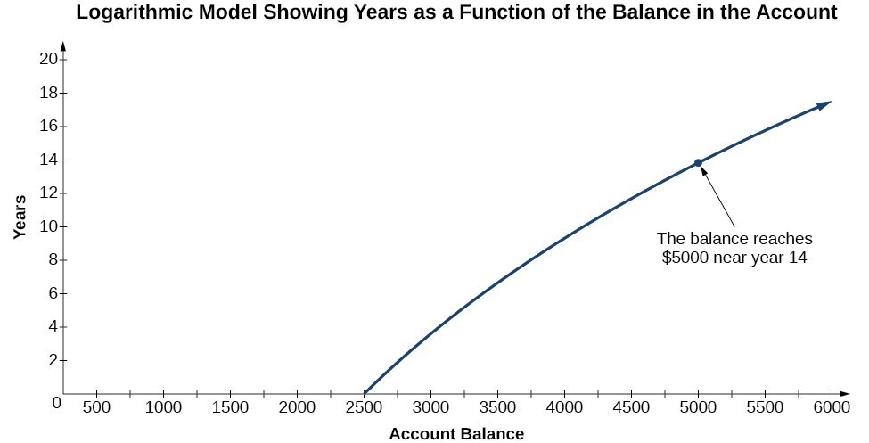
Figure 1
In this section we will discuss the values for which a logarithmic function is defined, and then turn our attention to graphing the family of logarithmic functions.
Before working with graphs, we will take a look at the domain (the set of input values) for which the logarithmic function is defined.
Recall that the exponential function is defined as [latex]y={b}^{x}\\[/latex] for any real number x and constant [latex]b>0\\[/latex], [latex]b\ne 1\\[/latex], where
In the last section we learned that the logarithmic function [latex]y={\mathrm{log}}_{b}\left(x\right)\\[/latex] is the inverse of the exponential function [latex]y={b}^{x}\\[/latex]. So, as inverse functions:
Transformations of the parent function [latex]y={\mathrm{log}}_{b}\left(x\right)\\[/latex] behave similarly to those of other functions. Just as with other parent functions, we can apply the four types of transformations—shifts, stretches, compressions, and reflections—to the parent function without loss of shape.
In Graphs of Exponential Functions we saw that certain transformations can change the range of [latex]y={b}^{x}\\[/latex]. Similarly, applying transformations to the parent function [latex]y={\mathrm{log}}_{b}\left(x\right)\\[/latex] can change the domain. When finding the domain of a logarithmic function, therefore, it is important to remember that the domain consists only of positive real numbers. That is, the argument of the logarithmic function must be greater than zero.
For example, consider [latex]f\left(x\right)={\mathrm{log}}_{4}\left(2x - 3\right)\\[/latex]. This function is defined for any values of x such that the argument, in this case [latex]2x - 3\\[/latex], is greater than zero. To find the domain, we set up an inequality and solve for x:
In interval notation, the domain of [latex]f\left(x\right)={\mathrm{log}}_{4}\left(2x - 3\right)\\[/latex] is [latex]\left(1.5,\infty \right)\\[/latex].
What is the domain of [latex]f\left(x\right)={\mathrm{log}}_{2}\left(x+3\right)\\[/latex]?
The logarithmic function is defined only when the input is positive, so this function is defined when [latex]x+3>0\\[/latex]. Solving this inequality,
The domain of [latex]f\left(x\right)={\mathrm{log}}_{2}\left(x+3\right)\\[/latex] is [latex]\left(-3,\infty \right)\\[/latex].
What is the domain of [latex]f\left(x\right)={\mathrm{log}}_{5}\left(x - 2\right)+1\\[/latex]?
What is the domain of [latex]f\left(x\right)=\mathrm{log}\left(5 - 2x\right)\\[/latex]?
The logarithmic function is defined only when the input is positive, so this function is defined when [latex]5 - 2x>0\\[/latex]. Solving this inequality,
The domain of [latex]f\left(x\right)=\mathrm{log}\left(5 - 2x\right)\\[/latex] is [latex]\left(-\infty ,\frac{5}{2}\right)\\[/latex].
What is the domain of [latex]f\left(x\right)=\mathrm{log}\left(x - 5\right)+2\\[/latex]?
Now that we have a feel for the set of values for which a logarithmic function is defined, we move on to graphing logarithmic functions. The family of logarithmic functions includes the parent function [latex]y={\mathrm{log}}_{b}\left(x\right)\\[/latex] along with all its transformations: shifts, stretches, compressions, and reflections.
We begin with the parent function [latex]y={\mathrm{log}}_{b}\left(x\right)\\[/latex]. Because every logarithmic function of this form is the inverse of an exponential function with the form [latex]y={b}^{x}\\[/latex], their graphs will be reflections of each other across the line [latex]y=x\\[/latex]. To illustrate this, we can observe the relationship between the input and output values of [latex]y={2}^{x}\\[/latex] and its equivalent [latex]x={\mathrm{log}}_{2}\left(y\right)\\[/latex] in the table below.
| x | –3 | –2 | –1 | 0 | 1 | 2 | 3 |
| [latex]{2}^{x}=y\\[/latex] | [latex]\frac{1}{8}\\[/latex] | [latex]\frac{1}{4}\\[/latex] | [latex]\frac{1}{2}\\[/latex] | 1 | 2 | 4 | 8 |
| [latex]{\mathrm{log}}_{2}\left(y\right)=x\\[/latex] | –3 | –2 | –1 | 0 | 1 | 2 | 3 |
Using the inputs and outputs from the table above, we can build another table to observe the relationship between points on the graphs of the inverse functions [latex]f\left(x\right)={2}^{x}\\[/latex] and [latex]g\left(x\right)={\mathrm{log}}_{2}\left(x\right)\\[/latex].
| [latex]f\left(x\right)={2}^{x}\\[/latex] | [latex]\left(-3,\frac{1}{8}\right)\\[/latex] | [latex]\left(-2,\frac{1}{4}\right)\\[/latex] | [latex]\left(-1,\frac{1}{2}\right)\\[/latex] | [latex]\left(0,1\right)\\[/latex] | [latex]\left(1,2\right)\\[/latex] | [latex]\left(2,4\right)\\[/latex] | [latex]\left(3,8\right)\\[/latex] |
| [latex]g\left(x\right)={\mathrm{log}}_{2}\left(x\right)\\[/latex] | [latex]\left(\frac{1}{8},-3\right)\\[/latex] | [latex]\left(\frac{1}{4},-2\right)\\[/latex] | [latex]\left(\frac{1}{2},-1\right)\\[/latex] | [latex]\left(1,0\right)\\[/latex] | [latex]\left(2,1\right)\\[/latex] | [latex]\left(4,2\right)\\[/latex] | [latex]\left(8,3\right)\\[/latex] |
As we’d expect, the x– and y-coordinates are reversed for the inverse functions. The figure below shows the graph of f and g.
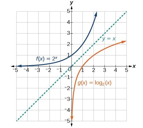
Figure 2. Notice that the graphs of [latex]f\left(x\right)={2}^{x}\\[/latex] and [latex]g\left(x\right)={\mathrm{log}}_{2}\left(x\right)\\[/latex] are reflections about the line y = x.
Observe the following from the graph:
For any real number x and constant b > 0, [latex]b\ne 1\\[/latex], we can see the following characteristics in the graph of [latex]f\left(x\right)={\mathrm{log}}_{b}\left(x\right)\\[/latex]:
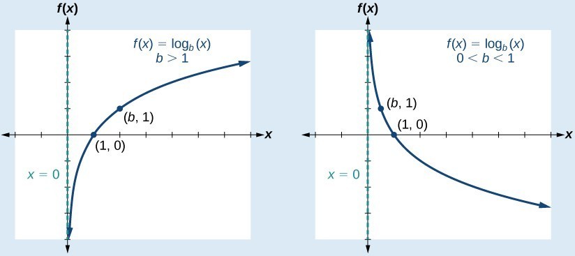
Figure 3
Figure 3 shows how changing the base b in [latex]f\left(x\right)={\mathrm{log}}_{b}\left(x\right)\\[/latex] can affect the graphs. Observe that the graphs compress vertically as the value of the base increases. (Note: recall that the function [latex]\mathrm{ln}\left(x\right)\\[/latex] has base [latex]e\approx \text{2}.\text{718.)}\\[/latex]
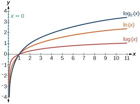
Figure 4. The graphs of three logarithmic functions with different bases, all greater than 1.
Graph [latex]f\left(x\right)={\mathrm{log}}_{5}\left(x\right)\\[/latex]. State the domain, range, and asymptote.
Before graphing, identify the behavior and key points for the graph.
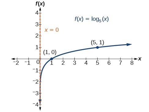
Figure 5. The domain is [latex]\left(0,\infty \right)\\[/latex], the range is [latex]\left(-\infty ,\infty \right)\\[/latex], and the vertical asymptote is x = 0.
Graph [latex]f\left(x\right)={\mathrm{log}}_{\frac{1}{5}}\left(x\right)\\[/latex]. State the domain, range, and asymptote.
As we mentioned in the beginning of the section, transformations of logarithmic graphs behave similarly to those of other parent functions. We can shift, stretch, compress, and reflect the parent function [latex]y={\mathrm{log}}_{b}\left(x\right)\\[/latex] without loss of shape.
When a constant c is added to the input of the parent function [latex]f\left(x\right)=\text{log}_{b}\left(x\right)\\[/latex], the result is a horizontal shift c units in the opposite direction of the sign on c. To visualize horizontal shifts, we can observe the general graph of the parent function [latex]f\left(x\right)={\mathrm{log}}_{b}\left(x\right)\\[/latex] and for c > 0 alongside the shift left, [latex]g\left(x\right)={\mathrm{log}}_{b}\left(x+c\right)\\[/latex], and the shift right, [latex]h\left(x\right)={\mathrm{log}}_{b}\left(x-c\right)\\[/latex].
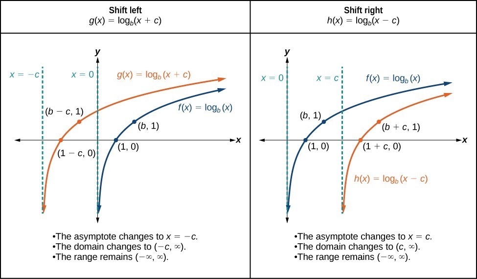
Figure 6
For any constant c, the function [latex]f\left(x\right)={\mathrm{log}}_{b}\left(x+c\right)\\[/latex]
Sketch the horizontal shift [latex]f\left(x\right)={\mathrm{log}}_{3}\left(x - 2\right)\\[/latex] alongside its parent function. Include the key points and asymptotes on the graph. State the domain, range, and asymptote.
Since the function is [latex]f\left(x\right)={\mathrm{log}}_{3}\left(x - 2\right)\\[/latex], we notice [latex]x+\left(-2\right)=x - 2\\[/latex].
Thus c = –2, so c < 0. This means we will shift the function [latex]f\left(x\right)={\mathrm{log}}_{3}\left(x\right)\\[/latex] right 2 units.
The vertical asymptote is [latex]x=-\left(-2\right)\\[/latex] or x = 2.
Consider the three key points from the parent function, [latex]\left(\frac{1}{3},-1\right)\\[/latex], [latex]\left(1,0\right)\\[/latex], and [latex]\left(3,1\right)\\[/latex].
The new coordinates are found by adding 2 to the x coordinates.
Label the points [latex]\left(\frac{7}{3},-1\right)\\[/latex], [latex]\left(3,0\right)\\[/latex], and [latex]\left(5,1\right)\\[/latex].
The domain is [latex]\left(2,\infty \right)\\[/latex], the range is [latex]\left(-\infty ,\infty \right)\\[/latex], and the vertical asymptote is x = 2.
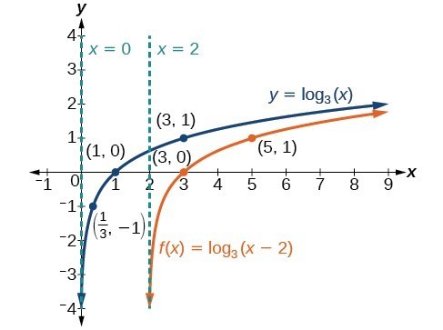
Figure 7
Sketch a graph of [latex]f\left(x\right)={\mathrm{log}}_{3}\left(x+4\right)\\[/latex] alongside its parent function. Include the key points and asymptotes on the graph. State the domain, range, and asymptote.
When a constant d is added to the parent function [latex]f\left(x\right)={\mathrm{log}}_{b}\left(x\right)\\[/latex], the result is a vertical shift d units in the direction of the sign on d. To visualize vertical shifts, we can observe the general graph of the parent function [latex]f\left(x\right)={\mathrm{log}}_{b}\left(x\right)\\[/latex] alongside the shift up, [latex]g\left(x\right)={\mathrm{log}}_{b}\left(x\right)+d\\[/latex] and the shift down, [latex]h\left(x\right)={\mathrm{log}}_{b}\left(x\right)-d\\[/latex].
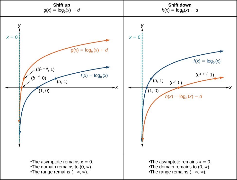
Figure 8
For any constant d, the function [latex]f\left(x\right)={\mathrm{log}}_{b}\left(x\right)+d\\[/latex]
Sketch a graph of [latex]f\left(x\right)={\mathrm{log}}_{3}\left(x\right)-2\\[/latex] alongside its parent function. Include the key points and asymptote on the graph. State the domain, range, and asymptote.
Since the function is [latex]f\left(x\right)={\mathrm{log}}_{3}\left(x\right)-2\\[/latex], we will notice d = –2. Thus d < 0.
This means we will shift the function [latex]f\left(x\right)={\mathrm{log}}_{3}\left(x\right)\\[/latex] down 2 units.
The vertical asymptote is x = 0.
Consider the three key points from the parent function, [latex]\left(\frac{1}{3},-1\right)\\[/latex], [latex]\left(1,0\right)\\[/latex], and [latex]\left(3,1\right)\\[/latex].
The new coordinates are found by subtracting 2 from the y coordinates.
Label the points [latex]\left(\frac{1}{3},-3\right)\\[/latex], [latex]\left(1,-2\right)\\[/latex], and [latex]\left(3,-1\right)\\[/latex].
The domain is [latex]\left(0,\infty \right)\\[/latex], the range is [latex]\left(-\infty ,\infty \right)\\[/latex], and the vertical asymptote is x = 0.
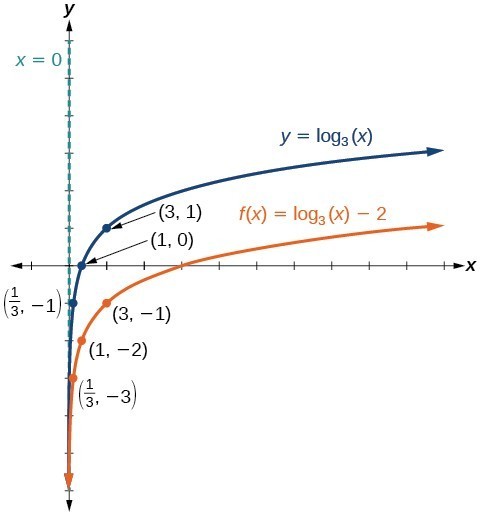
Figure 9. The domain is [latex]\left(0,\infty \right)\\[/latex], the range is [latex]\left(-\infty ,\infty \right)\\[/latex], and the vertical asymptote is x = 0.
Sketch a graph of [latex]f\left(x\right)={\mathrm{log}}_{2}\left(x\right)+2\\[/latex] alongside its parent function. Include the key points and asymptote on the graph. State the domain, range, and asymptote.
When the parent function [latex]f\left(x\right)={\mathrm{log}}_{b}\left(x\right)\\[/latex] is multiplied by a constant a > 0, the result is a vertical stretch or compression of the original graph. To visualize stretches and compressions, we set a > 1 and observe the general graph of the parent function [latex]f\left(x\right)={\mathrm{log}}_{b}\left(x\right)\\[/latex] alongside the vertical stretch, [latex]g\left(x\right)=a{\mathrm{log}}_{b}\left(x\right)\\[/latex] and the vertical compression, [latex]h\left(x\right)=\frac{1}{a}{\mathrm{log}}_{b}\left(x\right)\\[/latex].
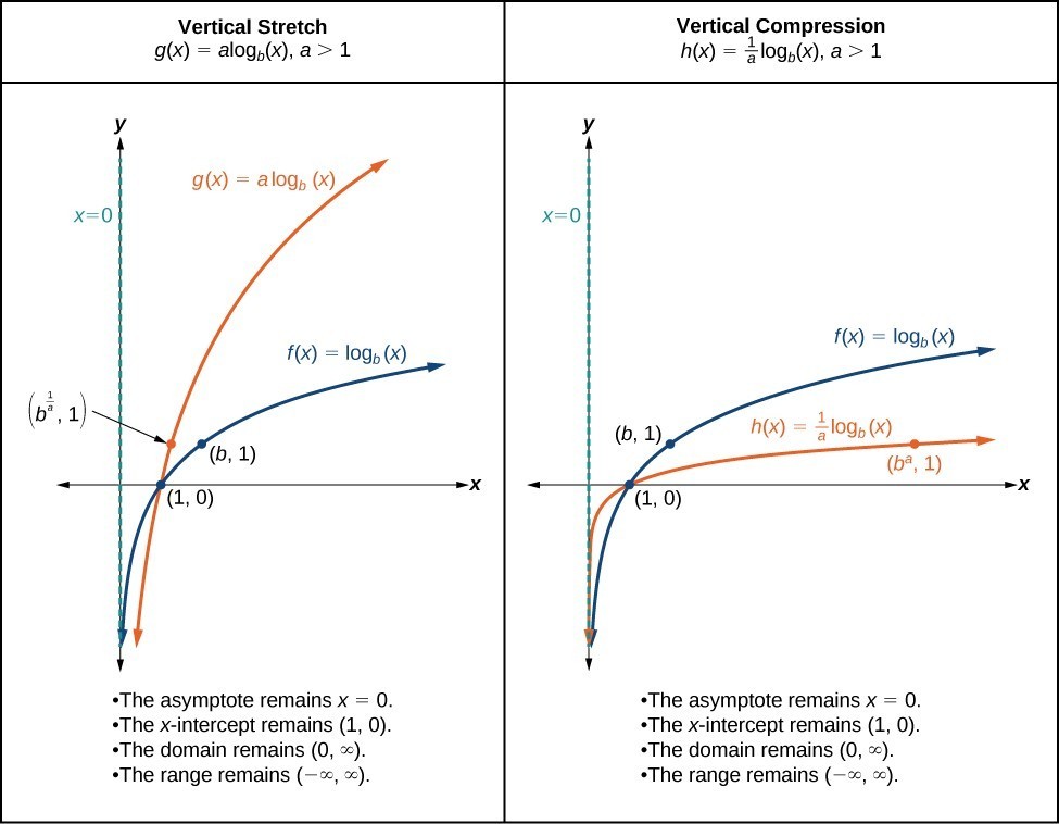
Figure 10
For any constant a > 1, the function [latex]f\left(x\right)=a{\mathrm{log}}_{b}\left(x\right)\\[/latex]
Sketch a graph of [latex]f\left(x\right)=2{\mathrm{log}}_{4}\left(x\right)\\[/latex] alongside its parent function. Include the key points and asymptote on the graph. State the domain, range, and asymptote.
Since the function is [latex]f\left(x\right)=2{\mathrm{log}}_{4}\left(x\right)\\[/latex], we will notice a = 2.
This means we will stretch the function [latex]f\left(x\right)={\mathrm{log}}_{4}\left(x\right)\\[/latex] by a factor of 2.
The vertical asymptote is x = 0.
Consider the three key points from the parent function, [latex]\left(\frac{1}{4},-1\right)\\[/latex], [latex]\left(1,0\right)\\[/latex], and [latex]\left(4,1\right)\\[/latex].
The new coordinates are found by multiplying the y coordinates by 2.
Label the points [latex]\left(\frac{1}{4},-2\right)\\[/latex], [latex]\left(1,0\right)\\[/latex], and [latex]\left(4,\text{2}\right)\\[/latex].
The domain is [latex]\left(0,\infty \right)\\[/latex], the range is [latex]\left(-\infty ,\infty \right)\\[/latex], and the vertical asymptote is x = 0.
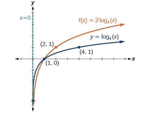
Figure 11. The domain is [latex]\left(0,\infty \right)\\[/latex], the range is [latex]\left(-\infty ,\infty \right)\\[/latex], and the vertical asymptote is x = 0.
Sketch a graph of [latex]f\left(x\right)=\frac{1}{2}{\mathrm{log}}_{4}\left(x\right)\\[/latex] alongside its parent function. Include the key points and asymptote on the graph. State the domain, range, and asymptote.
Sketch a graph of [latex]f\left(x\right)=5\mathrm{log}\left(x+2\right)\\[/latex]. State the domain, range, and asymptote.
Remember: what happens inside parentheses happens first. First, we move the graph left 2 units, then stretch the function vertically by a factor of 5. The vertical asymptote will be shifted to x = –2. The x-intercept will be [latex]\left(-1,0\right)\\[/latex]. The domain will be [latex]\left(-2,\infty \right)\\[/latex]. Two points will help give the shape of the graph: [latex]\left(-1,0\right)\\[/latex] and [latex]\left(8,5\right)\\[/latex]. We chose x = 8 as the x-coordinate of one point to graph because when x = 8, x + 2 = 10, the base of the common logarithm.
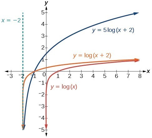
Figure 12. The domain is [latex]\left(-2,\infty \right)\\[/latex], the range is [latex]\left(-\infty ,\infty \right)\\[/latex], and the vertical asymptote is x = –2.
Sketch a graph of the function [latex]f\left(x\right)=3\mathrm{log}\left(x - 2\right)+1\\[/latex]. State the domain, range, and asymptote.
When the parent function [latex]f\left(x\right)={\mathrm{log}}_{b}\left(x\right)\\[/latex] is multiplied by –1, the result is a reflection about the x-axis. When the input is multiplied by –1, the result is a reflection about the y-axis. To visualize reflections, we restrict b > 1, and observe the general graph of the parent function [latex]f\left(x\right)={\mathrm{log}}_{b}\left(x\right)\\[/latex] alongside the reflection about the x-axis, [latex]g\left(x\right)={\mathrm{-log}}_{b}\left(x\right)\\[/latex] and the reflection about the y-axis, [latex]h\left(x\right)={\mathrm{log}}_{b}\left(-x\right)\\[/latex].
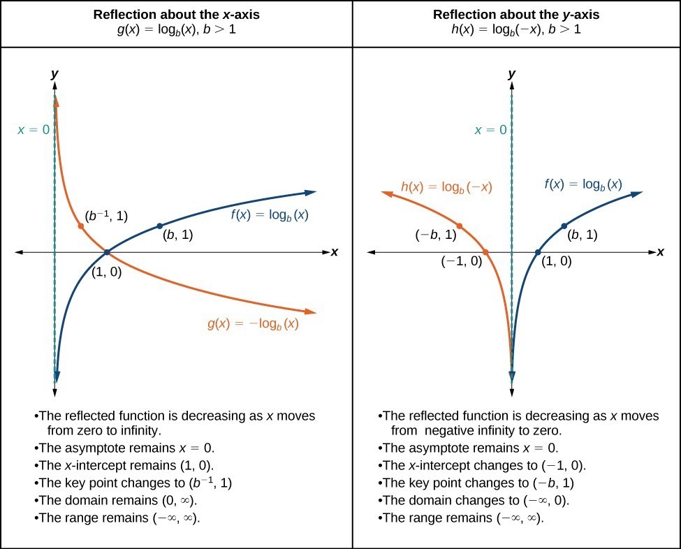
Figure 13
The function [latex]f\left(x\right)={\mathrm{-log}}_{b}\left(x\right)\\[/latex]
The function [latex]f\left(x\right)={\mathrm{log}}_{b}\left(-x\right)\\[/latex]
| [latex]\text{If }f\left(x\right)=-{\mathrm{log}}_{b}\left(x\right)\\[/latex] | [latex]\text{If }f\left(x\right)={\mathrm{log}}_{b}\left(-x\right)\\[/latex] |
|---|---|
| 1. Draw the vertical asymptote, x = 0. | 1. Draw the vertical asymptote, x = 0. |
| 2. Plot the x-intercept, [latex]\left(1,0\right)\\[/latex]. | 2. Plot the x-intercept, [latex]\left(1,0\right)\\[/latex]. |
| 3. Reflect the graph of the parent function [latex]f\left(x\right)={\mathrm{log}}_{b}\left(x\right)\\[/latex] about the x-axis. | 3. Reflect the graph of the parent function [latex]f\left(x\right)={\mathrm{log}}_{b}\left(x\right)\\[/latex] about the y-axis. |
| 4. Draw a smooth curve through the points. | 4. Draw a smooth curve through the points. |
| 5. State the domain, [latex]\left(0,\infty \right)[/latex], the range, [latex]\left(-\infty ,\infty \right)\\[/latex], and the vertical asymptote x = 0. | 5. State the domain, [latex]\left(-\infty ,0\right)\\[/latex], the range, [latex]\left(-\infty ,\infty \right)\\[/latex], and the vertical asymptote x = 0. |
Sketch a graph of [latex]f\left(x\right)=\mathrm{log}\left(-x\right)\\[/latex] alongside its parent function. Include the key points and asymptote on the graph. State the domain, range, and asymptote.
Before graphing [latex]f\left(x\right)=\mathrm{log}\left(-x\right)\\[/latex], identify the behavior and key points for the graph.

Figure 14. The domain is [latex]\left(-\infty ,0\right)\\[/latex], the range is [latex]\left(-\infty ,\infty \right)\\[/latex], and the vertical asymptote is x = 0.
Graph [latex]f\left(x\right)=-\mathrm{log}\left(-x\right)\\[/latex]. State the domain, range, and asymptote.
Solve [latex]4\mathrm{ln}\left(x\right)+1=-2\mathrm{ln}\left(x - 1\right)\\[/latex] graphically. Round to the nearest thousandth.
Press [Y=] and enter [latex]4\mathrm{ln}\left(x\right)+1\\[/latex] next to Y1=. Then enter [latex]-2\mathrm{ln}\left(x - 1\right)\\[/latex] next to Y2=. For a window, use the values 0 to 5 for x and –10 to 10 for y. Press [GRAPH]. The graphs should intersect somewhere a little to right of x = 1.
For a better approximation, press [2ND] then [CALC]. Select [5: intersect] and press [ENTER] three times. The x-coordinate of the point of intersection is displayed as 1.3385297. (Your answer may be different if you use a different window or use a different value for Guess?) So, to the nearest thousandth, [latex]x\approx 1.339\\[/latex].
Solve [latex]5\mathrm{log}\left(x+2\right)=4-\mathrm{log}\left(x\right)\\[/latex] graphically. Round to the nearest thousandth.
Now that we have worked with each type of translation for the logarithmic function, we can summarize each in the table below to arrive at the general equation for translating exponential functions.
| Translations of the Parent Function [latex]y={\mathrm{log}}_{b}\left(x\right)\\[/latex] | |
|---|---|
| Translation | Form |
Shift
| [latex]y={\mathrm{log}}_{b}\left(x+c\right)+d\\[/latex] |
Stretch and Compress
| [latex]y=a{\mathrm{log}}_{b}\left(x\right)\\[/latex] |
| Reflect about the x-axis | [latex]y=-{\mathrm{log}}_{b}\left(x\right)\\[/latex] |
| Reflect about the y-axis | [latex]y={\mathrm{log}}_{b}\left(-x\right)\\[/latex] |
| General equation for all translations | [latex]y=a{\mathrm{log}}_{b}\left(x+c\right)+d\\[/latex] |
All translations of the parent logarithmic function, [latex]y={\mathrm{log}}_{b}\left(x\right)\\[/latex], have the form
where the parent function, [latex]y={\mathrm{log}}_{b}\left(x\right),b>1\\[/latex], is
For [latex]f\left(x\right)=\mathrm{log}\left(-x\right)\\[/latex], the graph of the parent function is reflected about the y-axis.
What is the vertical asymptote of [latex]f\left(x\right)=-2{\mathrm{log}}_{3}\left(x+4\right)+5\\[/latex]?
The vertical asymptote is at x = –4.
The coefficient, the base, and the upward translation do not affect the asymptote. The shift of the curve 4 units to the left shifts the vertical asymptote to x = –4.
What is the vertical asymptote of [latex]f\left(x\right)=3+\mathrm{ln}\left(x - 1\right)\\[/latex]?
Find a possible equation for the common logarithmic function graphed in Figure 15.
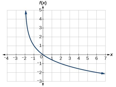
Figure 15
This graph has a vertical asymptote at x = –2 and has been vertically reflected. We do not know yet the vertical shift or the vertical stretch. We know so far that the equation will have form:
It appears the graph passes through the points [latex]\left(-1,1\right)\\[/latex] and [latex]\left(2,-1\right)\\[/latex]. Substituting [latex]\left(-1,1\right)\\[/latex],
Next, substituting in [latex]\left(2,-1\right)\\[/latex],
This gives us the equation [latex]f\left(x\right)=-\frac{2}{\mathrm{log}\left(4\right)}\mathrm{log}\left(x+2\right)+1\\[/latex].
We can verify this answer by comparing the function values in the table below with the points on the graph in Example 11.
| x | −1 | 0 | 1 | 2 | 3 |
| f(x) | 1 | 0 | −0.58496 | −1 | −1.3219 |
| x | 4 | 5 | 6 | 7 | 8 |
| f(x) | −1.5850 | −1.8074 | −2 | −2.1699 | −2.3219 |
Is it possible to tell the domain and range and describe the end behavior of a function just by looking at the graph?
Yes, if we know the function is a general logarithmic function. For example, look at the graph in Try It 11. The graph approaches x = –3 (or thereabouts) more and more closely, so x = –3 is, or is very close to, the vertical asymptote. It approaches from the right, so the domain is all points to the right, [latex]\left\{x|x>-3\right\}\\[/latex]. The range, as with all general logarithmic functions, is all real numbers. And we can see the end behavior because the graph goes down as it goes left and up as it goes right. The end behavior is that as [latex]x\to -{3}^{+},f\left(x\right)\to -\infty \\[/latex] and as [latex]x\to \infty ,f\left(x\right)\to \infty \\[/latex].
| General Form for the Translation of the Parent Logarithmic Function [latex]\text{ }f\left(x\right)={\mathrm{log}}_{b}\left(x\right)\\[/latex] | [latex] f\left(x\right)=a{\mathrm{log}}_{b}\left(x+c\right)+d\\[/latex] |
1. The inverse of every logarithmic function is an exponential function and vice-versa. What does this tell us about the relationship between the coordinates of the points on the graphs of each?
2. What type(s) of translation(s), if any, affect the range of a logarithmic function?
3. What type(s) of translation(s), if any, affect the domain of a logarithmic function?
4. Consider the general logarithmic function [latex]f\left(x\right)={\mathrm{log}}_{b}\left(x\right)\\[/latex]. Why can’t x be zero?
5. Does the graph of a general logarithmic function have a horizontal asymptote? Explain.
For the following exercises, state the domain and range of the function.
6. [latex]f\left(x\right)={\mathrm{log}}_{3}\left(x+4\right)\\[/latex]
7. [latex]h\left(x\right)=\mathrm{ln}\left(\frac{1}{2}-x\right)\\[/latex]
8. [latex]g\left(x\right)={\mathrm{log}}_{5}\left(2x+9\right)-2\\[/latex]
9. [latex]h\left(x\right)=\mathrm{ln}\left(4x+17\right)-5\\[/latex]
10. [latex]f\left(x\right)={\mathrm{log}}_{2}\left(12 - 3x\right)-3\\[/latex]
For the following exercises, state the domain and the vertical asymptote of the function.
11. [latex]f\left(x\right)={\mathrm{log}}_{b}\left(x - 5\right)\\[/latex]
12. [latex]g\left(x\right)=\mathrm{ln}\left(3-x\right)\\[/latex]
13. [latex]f\left(x\right)=\mathrm{log}\left(3x+1\right)\\[/latex]
14. [latex]f\left(x\right)=3\mathrm{log}\left(-x\right)+2\\[/latex]
15. [latex]g\left(x\right)=-\mathrm{ln}\left(3x+9\right)-7\\[/latex]
For the following exercises, state the domain, vertical asymptote, and end behavior of the function.
16. [latex]f\left(x\right)=\mathrm{ln}\left(2-x\right)\\[/latex]
17. [latex]f\left(x\right)=\mathrm{log}\left(x-\frac{3}{7}\right)\\[/latex]
18. [latex]h\left(x\right)=-\mathrm{log}\left(3x - 4\right)+3\\[/latex]
19. [latex]g\left(x\right)=\mathrm{ln}\left(2x+6\right)-5\\[/latex]
20. [latex]f\left(x\right)={\mathrm{log}}_{3}\left(15 - 5x\right)+6\\[/latex]
For the following exercises, state the domain, range, and x- and y-intercepts, if they exist. If they do not exist, write DNE.
21. [latex]h\left(x\right)={\mathrm{log}}_{4}\left(x - 1\right)+1\\[/latex]
22. [latex]f\left(x\right)=\mathrm{log}\left(5x+10\right)+3\\[/latex]
23. [latex]g\left(x\right)=\mathrm{ln}\left(-x\right)-2\\[/latex]
24. [latex]f\left(x\right)={\mathrm{log}}_{2}\left(x+2\right)-5\\[/latex]
25. [latex]h\left(x\right)=3\mathrm{ln}\left(x\right)-9\\[/latex]
For the following exercises, match each function in the graph below with the letter corresponding to its graph.

26. [latex]d\left(x\right)=\mathrm{log}\left(x\right)\\[/latex]
27. [latex]f\left(x\right)=\mathrm{ln}\left(x\right)\\[/latex]
28. [latex]g\left(x\right)={\mathrm{log}}_{2}\left(x\right)\\[/latex]
29. [latex]h\left(x\right)={\mathrm{log}}_{5}\left(x\right)\\[/latex]
30. [latex]j\left(x\right)={\mathrm{log}}_{25}\left(x\right)\\[/latex]
For the following exercises, match each function in the figure below with the letter corresponding to its graph.

31. [latex]f\left(x\right)={\mathrm{log}}_{\frac{1}{3}}\left(x\right)\\[/latex]
32. [latex]g\left(x\right)={\mathrm{log}}_{2}\left(x\right)\\[/latex]
33. [latex]h\left(x\right)={\mathrm{log}}_{\frac{3}{4}}\left(x\right)\\[/latex]
For the following exercises, sketch the graphs of each pair of functions on the same axis.
34. [latex]f\left(x\right)=\mathrm{log}\left(x\right)\\[/latex] and [latex]g\left(x\right)={10}^{x}\\[/latex]
35. [latex]f\left(x\right)=\mathrm{log}\left(x\right)\\[/latex] and [latex]g\left(x\right)={\mathrm{log}}_{\frac{1}{2}}\left(x\right)\\[/latex]
36. [latex]f\left(x\right)={\mathrm{log}}_{4}\left(x\right)\\[/latex] and [latex]g\left(x\right)=\mathrm{ln}\left(x\right)\\[/latex]
37. [latex]f\left(x\right)={e}^{x}\\[/latex] and [latex]g\left(x\right)=\mathrm{ln}\left(x\right)\\[/latex]
For the following exercises, match each function in the graph below with the letter corresponding to its graph.

38. [latex]f\left(x\right)={\mathrm{log}}_{4}\left(-x+2\right)\\[/latex]
39. [latex]g\left(x\right)=-{\mathrm{log}}_{4}\left(x+2\right)\\[/latex]
40. [latex]h\left(x\right)={\mathrm{log}}_{4}\left(x+2\right)\\[/latex]
For the following exercises, sketch the graph of the indicated function.
41. [latex]f\left(x\right)={\mathrm{log}}_{2}\left(x+2\right)\\[/latex]
42. [latex]f\left(x\right)=2\mathrm{log}\left(x\right)\\[/latex]
43. [latex]f\left(x\right)=\mathrm{ln}\left(-x\right)\\[/latex]
44. [latex]g\left(x\right)=\mathrm{log}\left(4x+16\right)+4\\[/latex]
45. [latex]g\left(x\right)=\mathrm{log}\left(6 - 3x\right)+1\\[/latex]
46. [latex]h\left(x\right)=-\frac{1}{2}\mathrm{ln}\left(x+1\right)-3\\[/latex]
For the following exercises, write a logarithmic equation corresponding to the graph shown.
47. Use [latex]y={\mathrm{log}}_{2}\left(x\right)\\[/latex] as the parent function.

48. Use [latex]f\left(x\right)={\mathrm{log}}_{3}\left(x\right)\\[/latex] as the parent function.

49. Use [latex]f\left(x\right)={\mathrm{log}}_{4}\left(x\right)\\[/latex] as the parent function.

50. Use [latex]f\left(x\right)={\mathrm{log}}_{5}\left(x\right)\\[/latex] as the parent function.

For the following exercises, use a graphing calculator to find approximate solutions to each equation.
51. [latex]\mathrm{log}\left(x - 1\right)+2=\mathrm{ln}\left(x - 1\right)+2\\[/latex]
52. [latex]\mathrm{log}\left(2x - 3\right)+2=-\mathrm{log}\left(2x - 3\right)+5\\[/latex]
53. [latex]\mathrm{ln}\left(x - 2\right)=-\mathrm{ln}\left(x+1\right)\\[/latex]
54. [latex]2\mathrm{ln}\left(5x+1\right)=\frac{1}{2}\mathrm{ln}\left(-5x\right)+1\\[/latex]
55. [latex]\frac{1}{3}\mathrm{log}\left(1-x\right)=\mathrm{log}\left(x+1\right)+\frac{1}{3}\\[/latex]
56. Let b be any positive real number such that [latex]b\ne 1\\[/latex]. What must [latex]{\mathrm{log}}_{b}1\\[/latex] be equal to? Verify the result.
57. Explore and discuss the graphs of [latex]f\left(x\right)={\mathrm{log}}_{\frac{1}{2}}\left(x\right)\\[/latex] and [latex]g\left(x\right)=-{\mathrm{log}}_{2}\left(x\right)\\[/latex]. Make a conjecture based on the result.
58. Prove the conjecture made in the previous exercise.
59. What is the domain of the function [latex]f\left(x\right)=\mathrm{ln}\left(\frac{x+2}{x - 4}\right)\\[/latex]? Discuss the result.
60. Use properties of exponents to find the x-intercepts of the function [latex]f\left(x\right)=\mathrm{log}\left({x}^{2}+4x+4\right)\\[/latex] algebraically. Show the steps for solving, and then verify the result by graphing the function.
1. [latex]\left(2,\infty \right)\\[/latex]
2. [latex]\left(5,\infty \right)\\[/latex]
3. The domain is [latex]\left(0,\infty \right)\\[/latex], the range is [latex]\left(-\infty ,\infty \right)\\[/latex], and the vertical asymptote is x = 0.

4. The domain is [latex]\left(-4,\infty \right)\\[/latex], the range [latex]\left(-\infty ,\infty \right)\\[/latex], and the asymptote x = –4.

5. The domain is [latex]\left(0,\infty \right)\\[/latex], the range is [latex]\left(-\infty ,\infty \right)\\[/latex], and the vertical asymptote is x = 0.

6. The domain is [latex]\left(0,\infty \right)\\[/latex], the range is [latex]\left(-\infty ,\infty \right)\\[/latex], and the vertical asymptote is x = 0.

7. The domain is [latex]\left(2,\infty \right)\\[/latex], the range is [latex]\left(-\infty ,\infty \right)\\[/latex], and the vertical asymptote is x = 2.

8. The domain is [latex]\left(-\infty ,0\right)\\[/latex], the range is [latex]\left(-\infty ,\infty \right)\\[/latex], and the vertical asymptote is x = 0.

9. [latex]x\approx 3.049\\[/latex]
10. x = 1
11. [latex]f\left(x\right)=2\mathrm{ln}\left(x+3\right)-1\\[/latex]
1. Since the functions are inverses, their graphs are mirror images about the line y = x. So for every point [latex]\left(a,b\right)\\[/latex] on the graph of a logarithmic function, there is a corresponding point [latex]\left(b,a\right)\\[/latex] on the graph of its inverse exponential function.
3. Shifting the function right or left and reflecting the function about the y-axis will affect its domain.
5. No. A horizontal asymptote would suggest a limit on the range, and the range of any logarithmic function in general form is all real numbers.
7. Domain: [latex]\left(-\infty ,\frac{1}{2}\right)\\[/latex]; Range: [latex]\left(-\infty ,\infty \right)\\[/latex]
9. Domain: [latex]\left(-\frac{17}{4},\infty \right)\\[/latex]; Range: [latex]\left(-\infty ,\infty \right)\\[/latex]
11. Domain: [latex]\left(5,\infty \right)\\[/latex]; Vertical asymptote: x = 5
13. Domain: [latex]\left(-\frac{1}{3},\infty \right)\\[/latex]; Vertical asymptote: [latex]x=-\frac{1}{3}\\[/latex]
15. Domain: [latex]\left(-3,\infty \right)\\[/latex]; Vertical asymptote: x = –3
17. Domain: [latex]\left(\frac{3}{7},\infty \right)\\[/latex]; Vertical asymptote: [latex]x=\frac{3}{7}\\[/latex] ; End behavior: as [latex]x\to {\left(\frac{3}{7}\right)}^{+},f\left(x\right)\to -\infty \\[/latex] and as [latex]x\to \infty ,f\left(x\right)\to \infty \\[/latex]
19. Domain: [latex]\left(-3,\infty \right)\\[/latex] ; Vertical asymptote: x = –3; End behavior: as [latex]x\to -{3}^{+}\\[/latex] , [latex]f\left(x\right)\to -\infty \\[/latex] and as [latex]x\to \infty \\[/latex] , [latex]f\left(x\right)\to \infty \\[/latex]
21. Domain: [latex]\left(1,\infty \right)\\[/latex]; Range: [latex]\left(-\infty ,\infty \right)\\[/latex]; Vertical asymptote: x = 1; x-intercept: [latex]\left(\frac{5}{4},0\right)\\[/latex]; y-intercept: DNE
23. Domain: [latex]\left(-\infty ,0\right)\\[/latex]; Range: [latex]\left(-\infty ,\infty \right)\\[/latex]; Vertical asymptote: x = 0; x-intercept: [latex]\left(-{e}^{2},0\right)\\[/latex]; y-intercept: DNE
25. Domain: [latex]\left(0,\infty \right)\\[/latex]; Range: [latex]\left(-\infty ,\infty \right)\\[/latex]; Vertical asymptote: x = 0; x-intercept: [latex]\left({e}^{3},0\right)[/latex]; y-intercept: DNE
27. B
29. C
31. B
33. C
35.

37.

39. C
41.

43.

45.

47. [latex]f\left(x\right)={\mathrm{log}}_{2}\left(-\left(x - 1\right)\right)\\[/latex]
49. [latex]f\left(x\right)=3{\mathrm{log}}_{4}\left(x+2\right)\\[/latex]
51. x = 2
53. [latex]x\approx \text{2}\text{.303}\\[/latex]
55. [latex]x\approx -0.472\\[/latex]
57. The graphs of [latex]f\left(x\right)={\mathrm{log}}_{\frac{1}{2}}\left(x\right)\\[/latex] and [latex]g\left(x\right)=-{\mathrm{log}}_{2}\left(x\right)\\[/latex] appear to be the same; Conjecture: for any positive base [latex]b\ne 1\\[/latex], [latex]{\mathrm{log}}_{b}\left(x\right)=-{\mathrm{log}}_{\frac{1}{b}}\left(x\right)\\[/latex].
59. Recall that the argument of a logarithmic function must be positive, so we determine where [latex]\frac{x+2}{x - 4}>0\\[/latex] . From the graph of the function [latex]f\left(x\right)=\frac{x+2}{x - 4}\\[/latex], note that the graph lies above the x-axis on the interval [latex]\left(-\infty ,-2\right)\\[/latex] and again to the right of the vertical asymptote, that is [latex]\left(4,\infty \right)\\[/latex]. Therefore, the domain is [latex]\left(-\infty ,-2\right)\cup \left(4,\infty \right)\\[/latex].
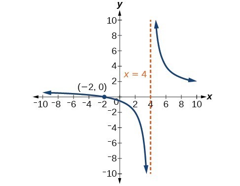
By the end of this lesson, you will be able to:
Figure 1. The pH of hydrochloric acid is tested with litmus paper. (credit: David Berardan)
In chemistry, pH is used as a measure of the acidity or alkalinity of a substance. The pH scale runs from 0 to 14. Substances with a pH less than 7 are considered acidic, and substances with a pH greater than 7 are said to be alkaline. Our bodies, for instance, must maintain a pH close to 7.35 in order for enzymes to work properly. To get a feel for what is acidic and what is alkaline, consider the following pH levels of some common substances:
To determine whether a solution is acidic or alkaline, we find its pH, which is a measure of the number of active positive hydrogen ions in the solution. The pH is defined by the following formula, where a is the concentration of hydrogen ion in the solution
The equivalence of [latex]-\mathrm{log}\left(\left[{H}^{+}\right]\right)\\[/latex] and [latex]\mathrm{log}\left(\frac{1}{\left[{H}^{+}\right]}\right)\\[/latex] is one of the logarithm properties we will examine in this section.
Recall that the logarithmic and exponential functions “undo” each other. This means that logarithms have similar properties to exponents. Some important properties of logarithms are given here. First, the following properties are easy to prove.
For example, [latex]{\mathrm{log}}_{5}1=0[/latex] since [latex]{5}^{0}=1\\[/latex]. And [latex]{\mathrm{log}}_{5}5=1\\[/latex] since [latex]{5}^{1}=5\\[/latex].
Next, we have the inverse property.
For example, to evaluate [latex]\mathrm{log}\left(100\right)\\[/latex], we can rewrite the logarithm as [latex]{\mathrm{log}}_{10}\left({10}^{2}\right)\\[/latex], and then apply the inverse property [latex]{\mathrm{log}}_{b}\left({b}^{x}\right)=x\\[/latex] to get [latex]{\mathrm{log}}_{10}\left({10}^{2}\right)=2\\[/latex].
To evaluate [latex]{e}^{\mathrm{ln}\left(7\right)}\\[/latex], we can rewrite the logarithm as [latex]{e}^{{\mathrm{log}}_{e}7}\\[/latex], and then apply the inverse property [latex]{b}^{{\mathrm{log}}_{b}x}=x\\[/latex] to get [latex]{e}^{{\mathrm{log}}_{e}7}=7\\[/latex].
Finally, we have the one-to-one property.
We can use the one-to-one property to solve the equation [latex]{\mathrm{log}}_{3}\left(3x\right)={\mathrm{log}}_{3}\left(2x+5\right)\\[/latex] for x. Since the bases are the same, we can apply the one-to-one property by setting the arguments equal and solving for x:
But what about the equation [latex]{\mathrm{log}}_{3}\left(3x\right)+{\mathrm{log}}_{3}\left(2x+5\right)=2\\[/latex]? The one-to-one property does not help us in this instance. Before we can solve an equation like this, we need a method for combining terms on the left side of the equation.
Recall that we use the product rule of exponents to combine the product of exponents by adding: [latex]{x}^{a}{x}^{b}={x}^{a+b}\\[/latex]. We have a similar property for logarithms, called the product rule for logarithms, which says that the logarithm of a product is equal to a sum of logarithms. Because logs are exponents, and we multiply like bases, we can add the exponents. We will use the inverse property to derive the product rule below.
Given any real number x and positive real numbers M, N, and b, where [latex]b\ne 1\\[/latex], we will show
Let [latex]m={\mathrm{log}}_{b}M\\[/latex] and [latex]n={\mathrm{log}}_{b}N\\[/latex]. In exponential form, these equations are [latex]{b}^{m}=M\\[/latex] and [latex]{b}^{n}=N\\[/latex]. It follows that
Note that repeated applications of the product rule for logarithms allow us to simplify the logarithm of the product of any number of factors. For example, consider [latex]{\mathrm{log}}_{b}\left(wxyz\right)\\[/latex]. Using the product rule for logarithms, we can rewrite this logarithm of a product as the sum of logarithms of its factors:
The product rule for logarithms can be used to simplify a logarithm of a product by rewriting it as a sum of individual logarithms.
Expand [latex]{\mathrm{log}}_{3}\left(30x\left(3x+4\right)\right)\\[/latex].
We begin by factoring the argument completely, expressing 30 as a product of primes.
Next we write the equivalent equation by summing the logarithms of each factor.
For quotients, we have a similar rule for logarithms. Recall that we use the quotient rule of exponents to combine the quotient of exponents by subtracting: [latex]{x}^{\frac{a}{b}}={x}^{a-b}\\[/latex]. The quotient rule for logarithms says that the logarithm of a quotient is equal to a difference of logarithms. Just as with the product rule, we can use the inverse property to derive the quotient rule.
Given any real number x and positive real numbers M, N, and b, where [latex]b\ne 1\\[/latex], we will show
Let [latex]m={\mathrm{log}}_{b}M\\[/latex] and [latex]n={\mathrm{log}}_{b}N\\[/latex]. In exponential form, these equations are [latex]{b}^{m}=M\\[/latex] and [latex]{b}^{n}=N\\[/latex]. It follows that
For example, to expand [latex]\mathrm{log}\left(\frac{2{x}^{2}+6x}{3x+9}\right)\\[/latex], we must first express the quotient in lowest terms. Factoring and canceling we get,
Next we apply the quotient rule by subtracting the logarithm of the denominator from the logarithm of the numerator. Then we apply the product rule.
The quotient rule for logarithms can be used to simplify a logarithm or a quotient by rewriting it as the difference of individual logarithms.
Expand [latex]{\mathrm{log}}_{2}\left(\frac{15x\left(x - 1\right)}{\left(3x+4\right)\left(2-x\right)}\right)\\[/latex].
First we note that the quotient is factored and in lowest terms, so we apply the quotient rule.
Notice that the resulting terms are logarithms of products. To expand completely, we apply the product rule, noting that the prime factors of the factor 15 are 3 and 5.
There are exceptions to consider in this and later examples. First, because denominators must never be zero, this expression is not defined for [latex]x=-\frac{4}{3}\\[/latex] and x = 2. Also, since the argument of a logarithm must be positive, we note as we observe the expanded logarithm, that x > 0, x > 1, [latex]x>-\frac{4}{3}\\[/latex], and x < 2. Combining these conditions is beyond the scope of this section, and we will not consider them here or in subsequent exercises.
Expand [latex]{\mathrm{log}}_{3}\left(\frac{7{x}^{2}+21x}{7x\left(x - 1\right)\left(x - 2\right)}\right)\\[/latex].
We’ve explored the product rule and the quotient rule, but how can we take the logarithm of a power, such as [latex]{x}^{2}\\[/latex]? One method is as follows:
Notice that we used the product rule for logarithms to find a solution for the example above. By doing so, we have derived the power rule for logarithms, which says that the log of a power is equal to the exponent times the log of the base. Keep in mind that, although the input to a logarithm may not be written as a power, we may be able to change it to a power. For example,
The power rule for logarithms can be used to simplify the logarithm of a power by rewriting it as the product of the exponent times the logarithm of the base.
Expand [latex]{\mathrm{log}}_{2}{x}^{5}\\[/latex].
The argument is already written as a power, so we identify the exponent, 5, and the base, x, and rewrite the equivalent expression by multiplying the exponent times the logarithm of the base.
Expand [latex]{\mathrm{log}}_{3}\left(25\right)\\[/latex] using the power rule for logs.
Expressing the argument as a power, we get [latex]{\mathrm{log}}_{3}\left(25\right)={\mathrm{log}}_{3}\left({5}^{2}\right)\\[/latex].
Next we identify the exponent, 2, and the base, 5, and rewrite the equivalent expression by multiplying the exponent times the logarithm of the base.
Rewrite [latex]4\mathrm{ln}\left(x\right)\\[/latex] using the power rule for logs to a single logarithm with a leading coefficient of 1.
Because the logarithm of a power is the product of the exponent times the logarithm of the base, it follows that the product of a number and a logarithm can be written as a power. For the expression [latex]4\mathrm{ln}\left(x\right)\\[/latex], we identify the factor, 4, as the exponent and the argument, x, as the base, and rewrite the product as a logarithm of a power:
[latex]4\mathrm{ln}\left(x\right)=\mathrm{ln}\left({x}^{4}\right)\\[/latex].
Rewrite [latex]2{\mathrm{log}}_{3}4\\[/latex] using the power rule for logs to a single logarithm with a leading coefficient of 1.
Taken together, the product rule, quotient rule, and power rule are often called “laws of logs.” Sometimes we apply more than one rule in order to simplify an expression. For example:
We can use the power rule to expand logarithmic expressions involving negative and fractional exponents. Here is an alternate proof of the quotient rule for logarithms using the fact that a reciprocal is a negative power:
We can also apply the product rule to express a sum or difference of logarithms as the logarithm of a product.
With practice, we can look at a logarithmic expression and expand it mentally, writing the final answer. Remember, however, that we can only do this with products, quotients, powers, and roots—never with addition or subtraction inside the argument of the logarithm.
Rewrite [latex]\mathrm{ln}\left(\frac{{x}^{4}y}{7}\right)\\[/latex] as a sum or difference of logs.
First, because we have a quotient of two expressions, we can use the quotient rule:
Then seeing the product in the first term, we use the product rule:
Finally, we use the power rule on the first term:
Expand [latex]\mathrm{log}\left(\sqrt{x}\right)\\[/latex].
[latex]\begin{cases}\mathrm{log}\left(\sqrt{x}\right)\hfill & =\mathrm{log}{x}^{\left(\frac{1}{2}\right)}\hfill \\ \hfill & =\frac{1}{2}\mathrm{log}x\hfill \end{cases}\\[/latex]
Can we expand [latex]\mathrm{ln}\left({x}^{2}+{y}^{2}\right)\\[/latex]?
No. There is no way to expand the logarithm of a sum or difference inside the argument of the logarithm.
Expand [latex]{\mathrm{log}}_{6}\left(\frac{64{x}^{3}\left(4x+1\right)}{\left(2x - 1\right)}\right)\\[/latex].
We can expand by applying the Product and Quotient Rules.
Expand [latex]\mathrm{ln}\left(\frac{\sqrt{\left(x - 1\right){\left(2x+1\right)}^{2}}}{\left({x}^{2}-9\right)}\right)\\[/latex].
We can use the rules of logarithms we just learned to condense sums, differences, and products with the same base as a single logarithm. It is important to remember that the logarithms must have the same base to be combined. We will learn later how to change the base of any logarithm before condensing.
Write [latex]{\mathrm{log}}_{3}\left(5\right)+{\mathrm{log}}_{3}\left(8\right)-{\mathrm{log}}_{3}\left(2\right)\\[/latex] as a single logarithm.
Using the product and quotient rules
This reduces our original expression to
Then, using the quotient rule
Condense [latex]\mathrm{log}3-\mathrm{log}4+\mathrm{log}5-\mathrm{log}6\\[/latex].
Condense [latex]{\mathrm{log}}_{2}\left({x}^{2}\right)+\frac{1}{2}{\mathrm{log}}_{2}\left(x - 1\right)-3{\mathrm{log}}_{2}\left({\left(x+3\right)}^{2}\right)\\[/latex].
We apply the power rule first:
Next we apply the product rule to the sum:
Finally, we apply the quotient rule to the difference:
Rewrite [latex]2\mathrm{log}x - 4\mathrm{log}\left(x+5\right)+\frac{1}{x}\mathrm{log}\left(3x+5\right)\\[/latex] as a single logarithm.
We apply the power rule first:
Next we apply the product rule to the sum:
Finally, we apply the quotient rule to the difference:
Rewrite [latex]\mathrm{log}\left(5\right)+0.5\mathrm{log}\left(x\right)-\mathrm{log}\left(7x - 1\right)+3\mathrm{log}\left(x - 1\right)\\[/latex] as a single logarithm.
Condense [latex]4\left(3\mathrm{log}\left(x\right)+\mathrm{log}\left(x+5\right)-\mathrm{log}\left(2x+3\right)\right)\\[/latex].
Recall that, in chemistry, [latex]\text{pH}=-\mathrm{log}\left[{H}^{+}\right]\\[/latex]. If the concentration of hydrogen ions in a liquid is doubled, what is the effect on pH?
Suppose C is the original concentration of hydrogen ions, and P is the original pH of the liquid. Then [latex]P=-\mathrm{log}\left(C\right)\\[/latex]. If the concentration is doubled, the new concentration is 2C. Then the pH of the new liquid is
Using the product rule of logs
Since [latex]P=-\mathrm{log}\left(C\right)\\[/latex], the new pH is
When the concentration of hydrogen ions is doubled, the pH decreases by about 0.301.
How does the pH change when the concentration of positive hydrogen ions is decreased by half?
Most calculators can evaluate only common and natural logs. In order to evaluate logarithms with a base other than 10 or [latex]e[/latex], we use the change-of-base formula to rewrite the logarithm as the quotient of logarithms of any other base; when using a calculator, we would change them to common or natural logs.
To derive the change-of-base formula, we use the one-to-one property and power rule for logarithms.
Given any positive real numbers M, b, and n, where [latex]n\ne 1 \\[/latex] and [latex]b\ne 1\\[/latex], we show
Let [latex]y={\mathrm{log}}_{b}M\\[/latex]. By taking the log base [latex]n[/latex] of both sides of the equation, we arrive at an exponential form, namely [latex]{b}^{y}=M\\[/latex]. It follows that
For example, to evaluate [latex]{\mathrm{log}}_{5}36\\[/latex] using a calculator, we must first rewrite the expression as a quotient of common or natural logs. We will use the common log.
The change-of-base formula can be used to evaluate a logarithm with any base.
For any positive real numbers M, b, and n, where [latex]n\ne 1 \\[/latex] and [latex]b\ne 1\\[/latex],
It follows that the change-of-base formula can be used to rewrite a logarithm with any base as the quotient of common or natural logs.
and
Change [latex]{\mathrm{log}}_{5}3\\[/latex] to a quotient of natural logarithms.
Because we will be expressing [latex]{\mathrm{log}}_{5}3\\[/latex] as a quotient of natural logarithms, the new base, n = e.
We rewrite the log as a quotient using the change-of-base formula. The numerator of the quotient will be the natural log with argument 3. The denominator of the quotient will be the natural log with argument 5.
Change [latex]{\mathrm{log}}_{0.5}8\\[/latex] to a quotient of natural logarithms.
Can we change common logarithms to natural logarithms?
Yes. Remember that [latex]\mathrm{log}9\\[/latex] means [latex]{\text{log}}_{\text{10}}\text{9}\\[/latex]. So, [latex]\mathrm{log}9=\frac{\mathrm{ln}9}{\mathrm{ln}10}\\[/latex].
Evaluate [latex]{\mathrm{log}}_{2}\left(10\right)\\[/latex] using the change-of-base formula with a calculator.
According to the change-of-base formula, we can rewrite the log base 2 as a logarithm of any other base. Since our calculators can evaluate the natural log, we might choose to use the natural logarithm, which is the log base e.
Evaluate [latex]{\mathrm{log}}_{5}\left(100\right)\\[/latex] using the change-of-base formula.
| The Product Rule for Logarithms | [latex]{\mathrm{log}}_{b}\left(MN\right)={\mathrm{log}}_{b}\left(M\right)+{\mathrm{log}}_{b}\left(N\right)\\[/latex] |
| The Quotient Rule for Logarithms | [latex]{\mathrm{log}}_{b}\left(\frac{M}{N}\right)={\mathrm{log}}_{b}M-{\mathrm{log}}_{b}N\\[/latex] |
| The Power Rule for Logarithms | [latex]{\mathrm{log}}_{b}\left({M}^{n}\right)=n{\mathrm{log}}_{b}M\\[/latex] |
| The Change-of-Base Formula | [latex]{\mathrm{log}}_{b}M\text{=}\frac{{\mathrm{log}}_{n}M}{{\mathrm{log}}_{n}b}\text{ }n>0,n\ne 1,b\ne 1\\[/latex] |
1. How does the power rule for logarithms help when solving logarithms with the form [latex]{\mathrm{log}}_{b}\left(\sqrt[n]{x}\right)\\[/latex]?
2. What does the change-of-base formula do? Why is it useful when using a calculator?
For the following exercises, expand each logarithm as much as possible. Rewrite each expression as a sum, difference, or product of logs.
3. [latex]{\mathrm{log}}_{b}\left(7x\cdot 2y\right)\\[/latex]
4. [latex]\mathrm{ln}\left(3ab\cdot 5c\right)\\[/latex]
5. [latex]{\mathrm{log}}_{b}\left(\frac{13}{17}\right)\\[/latex]
6. [latex]{\mathrm{log}}_{4}\left(\frac{\text{ }\frac{x}{z}\text{ }}{w}\right)\\[/latex]
7. [latex]\mathrm{ln}\left(\frac{1}{{4}^{k}}\right)\\[/latex]
8. [latex]{\mathrm{log}}_{2}\left({y}^{x}\right)\\[/latex]
For the following exercises, condense to a single logarithm if possible.
9. [latex]\mathrm{ln}\left(7\right)+\mathrm{ln}\left(x\right)+\mathrm{ln}\left(y\right)\\[/latex]
10. [latex]{\mathrm{log}}_{3}\left(2\right)+{\mathrm{log}}_{3}\left(a\right)+{\mathrm{log}}_{3}\left(11\right)+{\mathrm{log}}_{3}\left(b\right)\\[/latex]
11. [latex]{\mathrm{log}}_{b}\left(28\right)-{\mathrm{log}}_{b}\left(7\right)\\[/latex]
12. [latex]\mathrm{ln}\left(a\right)-\mathrm{ln}\left(d\right)-\mathrm{ln}\left(c\right)\\[/latex]
13. [latex]-{\mathrm{log}}_{b}\left(\frac{1}{7}\right)\\[/latex]
14. [latex]\frac{1}{3}\mathrm{ln}\left(8\right)\\[/latex]
For the following exercises, use the properties of logarithms to expand each logarithm as much as possible. Rewrite each expression as a sum, difference, or product of logs.
15. [latex]\mathrm{log}\left(\frac{{x}^{15}{y}^{13}}{{z}^{19}}\right)\\[/latex]
16. [latex]\mathrm{ln}\left(\frac{{a}^{-2}}{{b}^{-4}{c}^{5}}\right)\\[/latex]
17. [latex]\mathrm{log}\left(\sqrt{{x}^{3}{y}^{-4}}\right)\\[/latex]
18. [latex]\mathrm{ln}\left(y\sqrt{\frac{y}{1-y}}\right)\\[/latex]
19. [latex]\mathrm{log}\left({x}^{2}{y}^{3}\sqrt[3]{{x}^{2}{y}^{5}}\right)\\[/latex]
For the following exercises, condense each expression to a single logarithm using the properties of logarithms.
20. [latex]\mathrm{log}\left(2{x}^{4}\right)+\mathrm{log}\left(3{x}^{5}\right)\\[/latex]
21. [latex]\mathrm{ln}\left(6{x}^{9}\right)-\mathrm{ln}\left(3{x}^{2}\right)\\[/latex]
22. [latex]2\mathrm{log}\left(x\right)+3\mathrm{log}\left(x+1\right)\\[/latex]
23. [latex]\mathrm{log}\left(x\right)-\frac{1}{2}\mathrm{log}\left(y\right)+3\mathrm{log}\left(z\right)\\[/latex]
24. [latex]4{\mathrm{log}}_{7}\left(c\right)+\frac{{\mathrm{log}}_{7}\left(a\right)}{3}+\frac{{\mathrm{log}}_{7}\left(b\right)}{3}\\[/latex]
For the following exercises, rewrite each expression as an equivalent ratio of logs using the indicated base.
25. [latex]{\mathrm{log}}_{7}\left(15\right)\\[/latex] to base e
26. [latex]{\mathrm{log}}_{14}\left(55.875\right)\\[/latex] to base 10
For the following exercises, suppose [latex]{\mathrm{log}}_{5}\left(6\right)=a\\[/latex] and [latex]{\mathrm{log}}_{5}\left(11\right)=b\\[/latex]. Use the change-of-base formula along with properties of logarithms to rewrite each expression in terms of a and b. Show the steps for solving.
27. [latex]{\mathrm{log}}_{11}\left(5\right)\\[/latex]
28. [latex]{\mathrm{log}}_{6}\left(55\right)\\[/latex]
29. [latex]{\mathrm{log}}_{11}\left(\frac{6}{11}\right)\\[/latex]
For the following exercises, use properties of logarithms to evaluate without using a calculator.
30. [latex]{\mathrm{log}}_{3}\left(\frac{1}{9}\right)-3{\mathrm{log}}_{3}\left(3\right)\\[/latex]
31. [latex]6{\mathrm{log}}_{8}\left(2\right)+\frac{{\mathrm{log}}_{8}\left(64\right)}{3{\mathrm{log}}_{8}\left(4\right)}\\[/latex]
32. [latex]2{\mathrm{log}}_{9}\left(3\right)-4{\mathrm{log}}_{9}\left(3\right)+{\mathrm{log}}_{9}\left(\frac{1}{729}\right)\\[/latex]
For the following exercises, use the change-of-base formula to evaluate each expression as a quotient of natural logs. Use a calculator to approximate each to five decimal places.
33. [latex]{\mathrm{log}}_{3}\left(22\right)\\[/latex]
34. [latex]{\mathrm{log}}_{8}\left(65\right)\\[/latex]
35. [latex]{\mathrm{log}}_{6}\left(5.38\right)\\[/latex]
36. [latex]{\mathrm{log}}_{4}\left(\frac{15}{2}\right)\\[/latex]
37. [latex]{\mathrm{log}}_{\frac{1}{2}}\left(4.7\right)\\[/latex]
38. Use the product rule for logarithms to find all x values such that [latex]{\mathrm{log}}_{12}\left(2x+6\right)+{\mathrm{log}}_{12}\left(x+2\right)=2\\[/latex]. Show the steps for solving.
39. Use the quotient rule for logarithms to find all x values such that [latex]{\mathrm{log}}_{6}\left(x+2\right)-{\mathrm{log}}_{6}\left(x - 3\right)=1\\[/latex]. Show the steps for solving.
40. Can the power property of logarithms be derived from the power property of exponents using the equation [latex]{b}^{x}=m?\\[/latex] If not, explain why. If so, show the derivation.
41. Prove that [latex]{\mathrm{log}}_{b}\left(n\right)=\frac{1}{{\mathrm{log}}_{n}\left(b\right)}\\[/latex] for any positive integers b > 1 and n > 1.
42. Does [latex]{\mathrm{log}}_{81}\left(2401\right)={\mathrm{log}}_{3}\left(7\right)\\[/latex]? Verify the claim algebraically.
1. [latex]{\mathrm{log}}_{b}2+{\mathrm{log}}_{b}2+{\mathrm{log}}_{b}2+{\mathrm{log}}_{b}k=3{\mathrm{log}}_{b}2+{\mathrm{log}}_{b}k\\[/latex]
2. [latex]{\mathrm{log}}_{3}\left(x+3\right)-{\mathrm{log}}_{3}\left(x - 1\right)-{\mathrm{log}}_{3}\left(x - 2\right)\\[/latex]
3. [latex]2\mathrm{ln}x\\[/latex]
4. [latex]-2\mathrm{ln}\left(x\right)\\[/latex]
5. [latex]{\mathrm{log}}_{3}16\\[/latex]
6. [latex]2\mathrm{log}x+3\mathrm{log}y - 4\mathrm{log}z\\[/latex]
7. [latex]\frac{2}{3}\mathrm{ln}x\\[/latex]
8. [latex]\frac{1}{2}\mathrm{ln}\left(x - 1\right)+\mathrm{ln}\left(2x+1\right)-\mathrm{ln}\left(x+3\right)-\mathrm{ln}\left(x - 3\right)\\[/latex]
9. [latex]\mathrm{log}\left(\frac{3\cdot 5}{4\cdot 6}\right)\\[/latex]; can also be written [latex]\mathrm{log}\left(\frac{5}{8}\right)\\[/latex] by reducing the fraction to lowest terms.
10. [latex]\mathrm{log}\left(\frac{5{\left(x - 1\right)}^{3}\sqrt{x}}{\left(7x - 1\right)}\right)\\[/latex]
11. [latex]\mathrm{log}\frac{{x}^{12}{\left(x+5\right)}^{4}}{{\left(2x+3\right)}^{4}}\\[/latex]; this answer could also be written [latex]\mathrm{log}{\left(\frac{{x}^{3}\left(x+5\right)}{\left(2x+3\right)}\right)}^{4}\\[/latex].
12. The pH increases by about 0.301.
13. [latex]\frac{\mathrm{ln}8}{\mathrm{ln}0.5}\\[/latex]
14. [latex]\frac{\mathrm{ln}100}{\mathrm{ln}5}\approx \frac{4.6051}{1.6094}=2.861\\[/latex]
1. Any root expression can be rewritten as an expression with a rational exponent so that the power rule can be applied, making the logarithm easier to calculate. Thus, [latex]{\mathrm{log}}_{b}\left({x}^{\frac{1}{n}}\right)=\frac{1}{n}{\mathrm{log}}_{b}\left(x\right)\\[/latex].
3. [latex]{\mathrm{log}}_{b}\left(2\right)+{\mathrm{log}}_{b}\left(7\right)+{\mathrm{log}}_{b}\left(x\right)+{\mathrm{log}}_{b}\left(y\right)\\[/latex]
5. [latex]{\mathrm{log}}_{b}\left(13\right)-{\mathrm{log}}_{b}\left(17\right)\\[/latex]
7. [latex]-k\mathrm{ln}\left(4\right)\\[/latex]
9. [latex]\mathrm{ln}\left(7xy\right)\\[/latex]
11. [latex]{\mathrm{log}}_{b}\left(4\right)\\[/latex]
13. [latex]{\text{log}}_{b}\left(7\right)\\[/latex]
15. [latex]15\mathrm{log}\left(x\right)+13\mathrm{log}\left(y\right)-19\mathrm{log}\left(z\right)\\[/latex]
17. [latex]\frac{3}{2}\mathrm{log}\left(x\right)-2\mathrm{log}\left(y\right)\\[/latex]
19. [latex]\frac{8}{3}\mathrm{log}\left(x\right)+\frac{14}{3}\mathrm{log}\left(y\right)\\[/latex]
21. [latex]\mathrm{ln}\left(2{x}^{7}\right)\\[/latex]
23. [latex]\mathrm{log}\left(\frac{x{z}^{3}}{\sqrt{y}}\right)\\[/latex]
25. [latex]{\mathrm{log}}_{7}\left(15\right)=\frac{\mathrm{ln}\left(15\right)}{\mathrm{ln}\left(7\right)}\\[/latex]
27. [latex]{\mathrm{log}}_{11}\left(5\right)=\frac{{\mathrm{log}}_{5}\left(5\right)}{{\mathrm{log}}_{5}\left(11\right)}=\frac{1}{b}\\[/latex]
29. [latex]{\mathrm{log}}_{11}\left(\frac{6}{11}\right)=\frac{{\mathrm{log}}_{5}\left(\frac{6}{11}\right)}{{\mathrm{log}}_{5}\left(11\right)}=\frac{{\mathrm{log}}_{5}\left(6\right)-{\mathrm{log}}_{5}\left(11\right)}{{\mathrm{log}}_{5}\left(11\right)}=\frac{a-b}{b}=\frac{a}{b}-1\\[/latex]
31. 3
33. 2.81359
35. 0.93913
37. –2.23266
39. x = 4; By the quotient rule: [latex]{\mathrm{log}}_{6}\left(x+2\right)-{\mathrm{log}}_{6}\left(x - 3\right)={\mathrm{log}}_{6}\left(\frac{x+2}{x - 3}\right)=1\\[/latex].
Rewriting as an exponential equation and solving for x:
[latex]\begin{cases}{6}^{1}\hfill & =\frac{x+2}{x - 3}\hfill \\ 0\hfill & =\frac{x+2}{x - 3}-6\hfill \\ 0\hfill & =\frac{x+2}{x - 3}-\frac{6\left(x - 3\right)}{\left(x - 3\right)}\hfill \\ 0\hfill & =\frac{x+2 - 6x+18}{x - 3}\hfill \\ 0\hfill & =\frac{x - 4}{x - 3}\hfill \\ \text{ }x\hfill & =4\hfill \end{cases}\\[/latex]
Checking, we find that [latex]{\mathrm{log}}_{6}\left(4+2\right)-{\mathrm{log}}_{6}\left(4 - 3\right)={\mathrm{log}}_{6}\left(6\right)-{\mathrm{log}}_{6}\left(1\right)\\[/latex] is defined, so x = 4.
41. Let b and n be positive integers greater than 1. Then, by the change-of-base formula, [latex]{\mathrm{log}}_{b}\left(n\right)=\frac{{\mathrm{log}}_{n}\left(n\right)}{{\mathrm{log}}_{n}\left(b\right)}=\frac{1}{{\mathrm{log}}_{n}\left(b\right)}\\[/latex].
By the end of this lesson, you will be able to:

Figure 1. Wild rabbits in Australia. The rabbit population grew so quickly in Australia that the event became known as the “rabbit plague.” (credit: Richard Taylor, Flickr)
In 1859, an Australian landowner named Thomas Austin released 24 rabbits into the wild for hunting. Because Australia had few predators and ample food, the rabbit population exploded. In fewer than ten years, the rabbit population numbered in the millions.
Uncontrolled population growth, as in the wild rabbits in Australia, can be modeled with exponential functions. Equations resulting from those exponential functions can be solved to analyze and make predictions about exponential growth. In this section, we will learn techniques for solving exponential functions.
The first technique involves two functions with like bases. Recall that the one-to-one property of exponential functions tells us that, for any real numbers b, S, and T, where [latex]b>0,\text{ }b\ne 1\\[/latex], [latex]{b}^{S}={b}^{T}\\[/latex] if and only if S = T.
In other words, when an exponential equation has the same base on each side, the exponents must be equal. This also applies when the exponents are algebraic expressions. Therefore, we can solve many exponential equations by using the rules of exponents to rewrite each side as a power with the same base. Then, we use the fact that exponential functions are one-to-one to set the exponents equal to one another, and solve for the unknown.
For example, consider the equation [latex]{3}^{4x - 7}=\frac{{3}^{2x}}{3}\\[/latex]. To solve for x, we use the division property of exponents to rewrite the right side so that both sides have the common base, 3. Then we apply the one-to-one property of exponents by setting the exponents equal to one another and solving for x:
For any algebraic expressions S and T, and any positive real number [latex]b\ne 1\\[/latex],
Solve [latex]{2}^{x - 1}={2}^{2x - 4}\\[/latex].
[latex]\begin{cases} {2}^{x - 1}={2}^{2x - 4}\hfill & \text{The common base is }2.\hfill \\ \text{ }x - 1=2x - 4\hfill & \text{By the one-to-one property the exponents must be equal}.\hfill \\ \text{ }x=3\hfill & \text{Solve for }x.\hfill \end{cases}\\[/latex]
Sometimes the common base for an exponential equation is not explicitly shown. In these cases, we simply rewrite the terms in the equation as powers with a common base, and solve using the one-to-one property.
For example, consider the equation [latex]256={4}^{x - 5}\\[/latex]. We can rewrite both sides of this equation as a power of 2. Then we apply the rules of exponents, along with the one-to-one property, to solve for x:
Solve [latex]{8}^{x+2}={16}^{x+1}\\[/latex].
[latex]\begin{cases}\text{ }{8}^{x+2}={16}^{x+1}\hfill & \hfill \\ {\left({2}^{3}\right)}^{x+2}={\left({2}^{4}\right)}^{x+1}\hfill & \text{Write }8\text{ and }16\text{ as powers of }2.\hfill \\ \text{ }{2}^{3x+6}={2}^{4x+4}\hfill & \text{To take a power of a power, multiply exponents}.\hfill \\ \text{ }3x+6=4x+4\hfill & \text{Use the one-to-one property to set the exponents equal}.\hfill \\ \text{ }x=2\hfill & \text{Solve for }x.\hfill \end{cases}\\[/latex]
Solve [latex]{2}^{5x}=\sqrt{2}\\[/latex].
[latex]\begin{cases}{2}^{5x}={2}^{\frac{1}{2}}\hfill & \text{Write the square root of 2 as a power of }2.\hfill \\ 5x=\frac{1}{2}\hfill & \text{Use the one-to-one property}.\hfill \\ x=\frac{1}{10}\hfill & \text{Solve for }x.\hfill \end{cases}\\[/latex]
Do all exponential equations have a solution? If not, how can we tell if there is a solution during the problem-solving process?
No. Recall that the range of an exponential function is always positive. While solving the equation, we may obtain an expression that is undefined.
Solve [latex]{3}^{x+1}=-2\\[/latex].
This equation has no solution. There is no real value of x that will make the equation a true statement because any power of a positive number is positive.
The figure below shows that the two graphs do not cross so the left side is never equal to the right side. Thus the equation has no solution.
Figure 1
Sometimes the terms of an exponential equation cannot be rewritten with a common base. In these cases, we solve by taking the logarithm of each side. Recall, since [latex]\mathrm{log}\left(a\right)=\mathrm{log}\left(b\right)\\[/latex] is equivalent to a = b, we may apply logarithms with the same base on both sides of an exponential equation.
Solve [latex]{5}^{x+2}={4}^{x}\\[/latex].
[latex]\begin{cases}\text{ }{5}^{x+2}={4}^{x}\hfill & \text{There is no easy way to get the powers to have the same base}.\hfill \\ \text{ }\mathrm{ln}{5}^{x+2}=\mathrm{ln}{4}^{x}\hfill & \text{Take ln of both sides}.\hfill \\ \text{ }\left(x+2\right)\mathrm{ln}5=x\mathrm{ln}4\hfill & \text{Use laws of logs}.\hfill \\ \text{ }x\mathrm{ln}5+2\mathrm{ln}5=x\mathrm{ln}4\hfill & \text{Use the distributive law}.\hfill \\ \text{ }x\mathrm{ln}5-x\mathrm{ln}4=-2\mathrm{ln}5\hfill & \text{Get terms containing }x\text{ on one side, terms without }x\text{ on the other}.\hfill \\ x\left(\mathrm{ln}5-\mathrm{ln}4\right)=-2\mathrm{ln}5\hfill & \text{On the left hand side, factor out an }x.\hfill \\ \text{ }x\mathrm{ln}\left(\frac{5}{4}\right)=\mathrm{ln}\left(\frac{1}{25}\right)\hfill & \text{Use the laws of logs}.\hfill \\ \text{ }x=\frac{\mathrm{ln}\left(\frac{1}{25}\right)}{\mathrm{ln}\left(\frac{5}{4}\right)}\hfill & \text{Divide by the coefficient of }x.\hfill \end{cases}\\[/latex]
Is there any way to solve [latex]{2}^{x}={3}^{x}\\[/latex]?
Yes. The solution is x = 0.
One common type of exponential equations are those with base e. This constant occurs again and again in nature, in mathematics, in science, in engineering, and in finance. When we have an equation with a base e on either side, we can use the natural logarithm to solve it.
Solve [latex]100=20{e}^{2t}\\[/latex].
[latex]\begin{cases}100\hfill & =20{e}^{2t}\hfill & \hfill \\ 5\hfill & ={e}^{2t}\hfill & \text{Divide by the coefficient of the power}\text{.}\hfill \\ \mathrm{ln}5\hfill & =2t\hfill & \text{Take ln of both sides}\text{. Use the fact that }\mathrm{ln}\left(x\right)\text{ and }{e}^{x}\text{ are inverse functions}\text{.}\hfill \\ t\hfill & =\frac{\mathrm{ln}5}{2}\hfill & \text{Divide by the coefficient of }t\text{.}\hfill \end{cases}\\[/latex]
Using laws of logs, we can also write this answer in the form [latex]t=\mathrm{ln}\sqrt{5}\\[/latex]. If we want a decimal approximation of the answer, we use a calculator.
Does every equation of the form [latex]y=A{e}^{kt}\\[/latex] have a solution?
No. There is a solution when [latex]k\ne 0\\[/latex], and when y and A are either both 0 or neither 0, and they have the same sign. An example of an equation with this form that has no solution is [latex]2=-3{e}^{t}\\[/latex].
Solve [latex]4{e}^{2x}+5=12\\[/latex].
[latex]\begin{cases}4{e}^{2x}+5=12\hfill & \hfill \\ 4{e}^{2x}=7\hfill & \text{Combine like terms}.\hfill \\ {e}^{2x}=\frac{7}{4}\hfill & \text{Divide by the coefficient of the power}.\hfill \\ 2x=\mathrm{ln}\left(\frac{7}{4}\right)\hfill & \text{Take ln of both sides}.\hfill \\ x=\frac{1}{2}\mathrm{ln}\left(\frac{7}{4}\right)\hfill & \text{Solve for }x.\hfill \end{cases}\\[/latex]
Sometimes the methods used to solve an equation introduce an extraneous solution, which is a solution that is correct algebraically but does not satisfy the conditions of the original equation. One such situation arises in solving when the logarithm is taken on both sides of the equation. In such cases, remember that the argument of the logarithm must be positive. If the number we are evaluating in a logarithm function is negative, there is no output.
Solve [latex]{e}^{2x}-{e}^{x}=56\\[/latex].
[latex]\begin{cases}{e}^{2x}-{e}^{x}\hfill & =56\hfill & \hfill \\ {e}^{2x}-{e}^{x}-56\hfill & =0\hfill & \text{Get one side of the equation equal to zero}.\hfill \\ \left({e}^{x}+7\right)\left({e}^{x}-8\right)\hfill & =0\hfill & \text{Factor by the FOIL method}.\hfill \\ {e}^{x}+7\hfill & =0\text{ or }{e}^{x}-8=0 & \text{If a product is zero, then one factor must be zero}.\hfill \\ {e}^{x}\hfill & =-7{\text{ or e}}^{x}=8\hfill & \text{Isolate the exponentials}.\hfill \\ {e}^{x}\hfill & =8\hfill & \text{Reject the equation in which the power equals a negative number}.\hfill \\ x\hfill & =\mathrm{ln}8\hfill & \text{Solve the equation in which the power equals a positive number}.\hfill \end{cases}\\[/latex]
When we plan to use factoring to solve a problem, we always get zero on one side of the equation, because zero has the unique property that when a product is zero, one or both of the factors must be zero. We reject the equation [latex]{e}^{x}=-7\\[/latex] because a positive number never equals a negative number. The solution [latex]x=\mathrm{ln}\left(-7\right)\\[/latex] is not a real number, and in the real number system this solution is rejected as an extraneous solution.
Does every logarithmic equation have a solution?
No. Keep in mind that we can only apply the logarithm to a positive number. Always check for extraneous solutions.
We have already seen that every logarithmic equation [latex]{\mathrm{log}}_{b}\left(x\right)=y\\[/latex] is equivalent to the exponential equation [latex]{b}^{y}=x\\[/latex]. We can use this fact, along with the rules of logarithms, to solve logarithmic equations where the argument is an algebraic expression.
For example, consider the equation [latex]{\mathrm{log}}_{2}\left(2\right)+{\mathrm{log}}_{2}\left(3x - 5\right)=3\\[/latex]. To solve this equation, we can use rules of logarithms to rewrite the left side in compact form and then apply the definition of logs to solve for x:
For any algebraic expression S and real numbers b and c, where [latex]b>0,\text{ }b\ne 1\\[/latex],
Solve [latex]2\mathrm{ln}x+3=7\\[/latex].
[latex]\begin{cases}2\mathrm{ln}x+3=7\hfill & \hfill \\ \text{ }2\mathrm{ln}x=4\hfill & \text{Subtract 3}.\hfill \\ \text{ }\mathrm{ln}x=2\hfill & \text{Divide by 2}.\hfill \\ \text{ }x={e}^{2}\hfill & \text{Rewrite in exponential form}.\hfill \end{cases}\\[/latex]
Solve [latex]2\mathrm{ln}\left(6x\right)=7\\[/latex].
[latex]\begin{cases}2\mathrm{ln}\left(6x\right)=7\hfill & \hfill \\ \text{ }\mathrm{ln}\left(6x\right)=\frac{7}{2}\hfill & \text{Divide by 2}.\hfill \\ \text{ }6x={e}^{\left(\frac{7}{2}\right)}\hfill & \text{Use the definition of }\mathrm{ln}.\hfill \\ \text{ }x=\frac{1}{6}{e}^{\left(\frac{7}{2}\right)}\hfill & \text{Divide by 6}.\hfill \end{cases}\\[/latex]
Solve [latex]\mathrm{ln}x=3\\[/latex].
[latex]\begin{cases}\mathrm{ln}x=3\hfill & \hfill \\ x={e}^{3}\hfill & \text{Use the definition of the natural logarithm}\text{.}\hfill \end{cases}\\[/latex]
Figure 2 represents the graph of the equation. On the graph, the x-coordinate of the point at which the two graphs intersect is close to 20. In other words [latex]{e}^{3}\approx 20\\[/latex]. A calculator gives a better approximation: [latex]{e}^{3}\approx 20.0855\\[/latex].
Use a graphing calculator to estimate the approximate solution to the logarithmic equation [latex]{2}^{x}=1000\\[/latex] to 2 decimal places.
As with exponential equations, we can use the one-to-one property to solve logarithmic equations. The one-to-one property of logarithmic functions tells us that, for any real numbers x > 0, S > 0, T > 0 and any positive real number b, where [latex]b\ne 1\\[/latex],
For example,
So, if [latex]x - 1=8\\[/latex], then we can solve for x, and we get x = 9. To check, we can substitute x = 9 into the original equation: [latex]{\mathrm{log}}_{2}\left(9 - 1\right)={\mathrm{log}}_{2}\left(8\right)=3\\[/latex]. In other words, when a logarithmic equation has the same base on each side, the arguments must be equal. This also applies when the arguments are algebraic expressions. Therefore, when given an equation with logs of the same base on each side, we can use rules of logarithms to rewrite each side as a single logarithm. Then we use the fact that logarithmic functions are one-to-one to set the arguments equal to one another and solve for the unknown.
For example, consider the equation [latex]\mathrm{log}\left(3x - 2\right)-\mathrm{log}\left(2\right)=\mathrm{log}\left(x+4\right)\\[/latex]. To solve this equation, we can use the rules of logarithms to rewrite the left side as a single logarithm, and then apply the one-to-one property to solve for x:
To check the result, substitute x = 10 into [latex]\mathrm{log}\left(3x - 2\right)-\mathrm{log}\left(2\right)=\mathrm{log}\left(x+4\right)\\[/latex].
For any algebraic expressions S and T and any positive real number b, where [latex]b\ne 1\\[/latex],
Note, when solving an equation involving logarithms, always check to see if the answer is correct or if it is an extraneous solution.
Solve [latex]\mathrm{ln}\left({x}^{2}\right)=\mathrm{ln}\left(2x+3\right)\\[/latex].
[latex]\begin{cases}\text{ }\mathrm{ln}\left({x}^{2}\right)=\mathrm{ln}\left(2x+3\right)\hfill & \hfill \\ \text{ }{x}^{2}=2x+3\hfill & \text{Use the one-to-one property of the logarithm}.\hfill \\ \text{ }{x}^{2}-2x - 3=0\hfill & \text{Get zero on one side before factoring}.\hfill \\ \left(x - 3\right)\left(x+1\right)=0\hfill & \text{Factor using FOIL}.\hfill \\ \text{ }x - 3=0\text{ or }x+1=0\hfill & \text{If a product is zero, one of the factors must be zero}.\hfill \\ \text{ }x=3\text{ or }x=-1\hfill & \text{Solve for }x.\hfill \end{cases}\\[/latex]
There are two solutions: x = 3 or x = –1. The solution x = –1 is negative, but it checks when substituted into the original equation because the argument of the logarithm functions is still positive.
In previous sections, we learned the properties and rules for both exponential and logarithmic functions. We have seen that any exponential function can be written as a logarithmic function and vice versa. We have used exponents to solve logarithmic equations and logarithms to solve exponential equations. We are now ready to combine our skills to solve equations that model real-world situations, whether the unknown is in an exponent or in the argument of a logarithm.
One such application is in science, in calculating the time it takes for half of the unstable material in a sample of a radioactive substance to decay, called its half-life. The table below lists the half-life for several of the more common radioactive substances.
| Substance | Use | Half-life |
|---|---|---|
| gallium-67 | nuclear medicine | 80 hours |
| cobalt-60 | manufacturing | 5.3 years |
| technetium-99m | nuclear medicine | 6 hours |
| americium-241 | construction | 432 years |
| carbon-14 | archeological dating | 5,715 years |
| uranium-235 | atomic power | 703,800,000 years |
We can see how widely the half-lives for these substances vary. Knowing the half-life of a substance allows us to calculate the amount remaining after a specified time. We can use the formula for radioactive decay:
where
How long will it take for ten percent of a 1000-gram sample of uranium-235 to decay?
[latex]\begin{cases}\text{ }y=\text{1000}e\frac{\mathrm{ln}\left(0.5\right)}{\text{703,800,000}}t\hfill & \hfill \\ \text{ }900=1000{e}^{\frac{\mathrm{ln}\left(0.5\right)}{\text{703,800,000}}t}\hfill & \text{After 10% decays, 900 grams are left}.\hfill \\ \text{ }0.9={e}^{\frac{\mathrm{ln}\left(0.5\right)}{\text{703,800,000}}t}\hfill & \text{Divide by 1000}.\hfill \\ \mathrm{ln}\left(0.9\right)=\mathrm{ln}\left({e}^{\frac{\mathrm{ln}\left(0.5\right)}{\text{703,800,000}}t}\right)\hfill & \text{Take ln of both sides}.\hfill \\ \mathrm{ln}\left(0.9\right)=\frac{\mathrm{ln}\left(0.5\right)}{\text{703,800,000}}t\hfill & \text{ln}\left({e}^{M}\right)=M\hfill \\ \text{ }\text{ }t=\text{703,800,000}\times \frac{\mathrm{ln}\left(0.9\right)}{\mathrm{ln}\left(0.5\right)}\text{years}\begin{cases}{cccc}& & & \end{cases}\hfill & \text{Solve for }t.\hfill \\ \text{ }\text{ }t\approx \text{106,979,777 years}\hfill & \hfill \end{cases}\\[/latex]
Ten percent of 1000 grams is 100 grams. If 100 grams decay, the amount of uranium-235 remaining is 900 grams.
How long will it take before twenty percent of our 1000-gram sample of uranium-235 has decayed?
| One-to-one property for exponential functions | For any algebraic expressions S and T and any positive real number b, where[latex]{b}^{S}={b}^{T}\\[/latex] if and only if S = T. |
| Definition of a logarithm | For any algebraic expression S and positive real numbers b and c, where [latex]b\ne 1\\[/latex],[latex]{\mathrm{log}}_{b}\left(S\right)=c\\[/latex] if and only if [latex]{b}^{c}=S\\[/latex]. |
| One-to-one property for logarithmic functions | For any algebraic expressions S and T and any positive real number b, where [latex]b\ne 1\\[/latex], [latex]{\mathrm{log}}_{b}S={\mathrm{log}}_{b}T\\[/latex] if and only if S = T. |
1. How can an exponential equation be solved?
2. When does an extraneous solution occur? How can an extraneous solution be recognized?
3. When can the one-to-one property of logarithms be used to solve an equation? When can it not be used?
For the following exercises, use like bases to solve the exponential equation.
4. [latex]{4}^{-3v - 2}={4}^{-v}\\[/latex]
5. [latex]64\cdot {4}^{3x}=16\\[/latex]
6. [latex]{3}^{2x+1}\cdot {3}^{x}=243\\[/latex]
7. [latex]{2}^{-3n}\cdot \frac{1}{4}={2}^{n+2}\\[/latex]
8. [latex]625\cdot {5}^{3x+3}=125\\[/latex]
9. [latex]\frac{{36}^{3b}}{{36}^{2b}}={216}^{2-b}\\[/latex]
10. [latex]{\left(\frac{1}{64}\right)}^{3n}\cdot 8={2}^{6}\\[/latex]
For the following exercises, use logarithms to solve.
11. [latex]{9}^{x - 10}=1\\[/latex]
12. [latex]2{e}^{6x}=13\\[/latex]
13. [latex]{e}^{r+10}-10=-42\\[/latex]
14. [latex]2\cdot {10}^{9a}=29\\[/latex]
15. [latex]-8\cdot {10}^{p+7}-7=-24\\[/latex]
16. [latex]7{e}^{3n - 5}+5=-89\\[/latex]
17. [latex]{e}^{-3k}+6=44\\[/latex]
18. [latex]-5{e}^{9x - 8}-8=-62\\[/latex]
19. [latex]-6{e}^{9x+8}+2=-74\\[/latex]
20. [latex]{2}^{x+1}={5}^{2x - 1}\\[/latex]
21. [latex]{e}^{2x}-{e}^{x}-132=0\\[/latex]
22. [latex]7{e}^{8x+8}-5=-95\\[/latex]
23. [latex]10{e}^{8x+3}+2=8\\[/latex]
24. [latex]4{e}^{3x+3}-7=53\\[/latex]
25. [latex]8{e}^{-5x - 2}-4=-90\\[/latex]
26. [latex]{3}^{2x+1}={7}^{x - 2}\\[/latex]
27. [latex]{e}^{2x}-{e}^{x}-6=0\\[/latex]
28. [latex]3{e}^{3 - 3x}+6=-31\\[/latex]
For the following exercises, use the definition of a logarithm to rewrite the equation as an exponential equation.
29. [latex]\mathrm{log}\left(\frac{1}{100}\right)=-2\\[/latex]
30. [latex]{\mathrm{log}}_{324}\left(18\right)=\frac{1}{2}\\[/latex]
For the following exercises, use the definition of a logarithm to solve the equation.
31. [latex]5{\mathrm{log}}_{7}n=10\\[/latex]
32. [latex]-8{\mathrm{log}}_{9}x=16\\[/latex]
33. [latex]4+{\mathrm{log}}_{2}\left(9k\right)=2\\[/latex]
34. [latex]2\mathrm{log}\left(8n+4\right)+6=10\\[/latex]
35. [latex]10 - 4\mathrm{ln}\left(9 - 8x\right)=6\\[/latex]
For the following exercises, use the one-to-one property of logarithms to solve.
36. [latex]\mathrm{ln}\left(10 - 3x\right)=\mathrm{ln}\left(-4x\right)\\[/latex]
37. [latex]{\mathrm{log}}_{13}\left(5n - 2\right)={\mathrm{log}}_{13}\left(8 - 5n\right)\\[/latex]
38. [latex]\mathrm{log}\left(x+3\right)-\mathrm{log}\left(x\right)=\mathrm{log}\left(74\right)\\[/latex]
39. [latex]\mathrm{ln}\left(-3x\right)=\mathrm{ln}\left({x}^{2}-6x\right)\\[/latex]
40. [latex]{\mathrm{log}}_{4}\left(6-m\right)={\mathrm{log}}_{4}3m\\[/latex]
41. [latex]\mathrm{ln}\left(x - 2\right)-\mathrm{ln}\left(x\right)=\mathrm{ln}\left(54\right)\\[/latex]
42. [latex]{\mathrm{log}}_{9}\left(2{n}^{2}-14n\right)={\mathrm{log}}_{9}\left(-45+{n}^{2}\right)\\[/latex]
43. [latex]\mathrm{ln}\left({x}^{2}-10\right)+\mathrm{ln}\left(9\right)=\mathrm{ln}\left(10\right)\\[/latex]
For the following exercises, solve each equation for x.
44. [latex]\mathrm{log}\left(x+12\right)=\mathrm{log}\left(x\right)+\mathrm{log}\left(12\right)\\[/latex]
45. [latex]\mathrm{ln}\left(x\right)+\mathrm{ln}\left(x - 3\right)=\mathrm{ln}\left(7x\right)\\[/latex]
46. [latex]{\mathrm{log}}_{2}\left(7x+6\right)=3\\[/latex]
47. [latex]\mathrm{ln}\left(7\right)+\mathrm{ln}\left(2 - 4{x}^{2}\right)=\mathrm{ln}\left(14\right)\\[/latex]
48. [latex]{\mathrm{log}}_{8}\left(x+6\right)-{\mathrm{log}}_{8}\left(x\right)={\mathrm{log}}_{8}\left(58\right)\\[/latex]
49. [latex]\mathrm{ln}\left(3\right)-\mathrm{ln}\left(3 - 3x\right)=\mathrm{ln}\left(4\right)\\[/latex]
50. [latex]{\mathrm{log}}_{3}\left(3x\right)-{\mathrm{log}}_{3}\left(6\right)={\mathrm{log}}_{3}\left(77\right)\\[/latex]
For the following exercises, solve the equation for x, if there is a solution. Then graph both sides of the equation, and observe the point of intersection (if it exists) to verify the solution.
51. [latex]{\mathrm{log}}_{9}\left(x\right)-5=-4\\[/latex]
52. [latex]{\mathrm{log}}_{3}\left(x\right)+3=2\\[/latex]
53. [latex]\mathrm{ln}\left(3x\right)=2\\[/latex]
54. [latex]\mathrm{ln}\left(x - 5\right)=1\\[/latex]
55. [latex]\mathrm{log}\left(4\right)+\mathrm{log}\left(-5x\right)=2\\[/latex]
56. [latex]-7+{\mathrm{log}}_{3}\left(4-x\right)=-6\\[/latex]
57. [latex]\mathrm{ln}\left(4x - 10\right)-6=-5\\[/latex]
58. [latex]\mathrm{log}\left(4 - 2x\right)=\mathrm{log}\left(-4x\right)\\[/latex]
59. [latex]{\mathrm{log}}_{11}\left(-2{x}^{2}-7x\right)={\mathrm{log}}_{11}\left(x - 2\right)\\[/latex]
60. [latex]\mathrm{ln}\left(2x+9\right)=\mathrm{ln}\left(-5x\right)\\[/latex]
61. [latex]{\mathrm{log}}_{9}\left(3-x\right)={\mathrm{log}}_{9}\left(4x - 8\right)\\[/latex]
62. [latex]\mathrm{log}\left({x}^{2}+13\right)=\mathrm{log}\left(7x+3\right)\\[/latex]
63. [latex]\frac{3}{{\mathrm{log}}_{2}\left(10\right)}-\mathrm{log}\left(x - 9\right)=\mathrm{log}\left(44\right)\\[/latex]
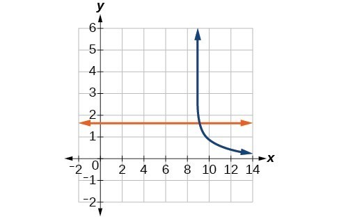
64. [latex]\mathrm{ln}\left(x\right)-\mathrm{ln}\left(x+3\right)=\mathrm{ln}\left(6\right)\\[/latex]
For the following exercises, solve for the indicated value, and graph the situation showing the solution point.
65. An account with an initial deposit of $6,500 earns 7.25% annual interest, compounded continuously. How much will the account be worth after 20 years?

66. The formula for measuring sound intensity in decibels D is defined by the equation [latex]D=10\mathrm{log}\left(\frac{I}{{I}_{0}}\right)\\[/latex], where I is the intensity of the sound in watts per square meter and [latex]{I}_{0}={10}^{-12}\\[/latex] is the lowest level of sound that the average person can hear. How many decibels are emitted from a jet plane with a sound intensity of [latex]8.3\cdot {10}^{2}\\[/latex] watts per square meter?
67. The population of a small town is modeled by the equation [latex]P=1650{e}^{0.5t}\\[/latex] where t is measured in years. In approximately how many years will the town’s population reach 20,000?
For the following exercises, solve each equation by rewriting the exponential expression using the indicated logarithm. Then use a calculator to approximate x to 3 decimal places.
68. [latex]1000{\left(1.03\right)}^{t}=5000\\[/latex] using the common log.
69. [latex]{e}^{5x}=17\\[/latex] using the natural log
70. [latex]3{\left(1.04\right)}^{3t}=8\\[/latex] using the common log
71. [latex]{3}^{4x - 5}=38\\[/latex] using the common log
72. [latex]50{e}^{-0.12t}=10\\[/latex] using the natural log
For the following exercises, use a calculator to solve the equation. Unless indicated otherwise, round all answers to the nearest ten-thousandth.
73. [latex]7{e}^{3x - 5}+7.9=47\\[/latex]
74. [latex]\mathrm{ln}\left(3\right)+\mathrm{ln}\left(4.4x+6.8\right)=2\\[/latex]
75. [latex]\mathrm{log}\left(-0.7x - 9\right)=1+5\mathrm{log}\left(5\right)\\[/latex]
76. Atmospheric pressure P in pounds per square inch is represented by the formula [latex]P=14.7{e}^{-0.21x}\\[/latex], where x is the number of miles above sea level. To the nearest foot, how high is the peak of a mountain with an atmospheric pressure of 8.369 pounds per square inch? (Hint: there are 5280 feet in a mile)
77. The magnitude M of an earthquake is represented by the equation [latex]M=\frac{2}{3}\mathrm{log}\left(\frac{E}{{E}_{0}}\right)\\[/latex] where E is the amount of energy released by the earthquake in joules and [latex]{E}_{0}={10}^{4.4}\\[/latex] is the assigned minimal measure released by an earthquake. To the nearest hundredth, what would the magnitude be of an earthquake releasing [latex]1.4\cdot {10}^{13}\\[/latex] joules of energy?
78. Use the definition of a logarithm along with the one-to-one property of logarithms to prove that [latex]{b}^{{\mathrm{log}}_{b}x}=x\\[/latex].
79. Recall the formula for continually compounding interest, [latex]y=A{e}^{kt}\\[/latex]. Use the definition of a logarithm along with properties of logarithms to solve the formula for time t such that t is equal to a single logarithm.
80. Recall the compound interest formula [latex]A=a{\left(1+\frac{r}{k}\right)}^{kt}\\[/latex]. Use the definition of a logarithm along with properties of logarithms to solve the formula for time t.
81. Newton’s Law of Cooling states that the temperature T of an object at any time t can be described by the equation [latex]T={T}_{s}+\left({T}_{0}-{T}_{s}\right){e}^{-kt}\\[/latex], where [latex]{T}_{s}\\[/latex] is the temperature of the surrounding environment, [latex]{T}_{0}\\[/latex] is the initial temperature of the object, and k is the cooling rate. Use the definition of a logarithm along with properties of logarithms to solve the formula for time t such that t is equal to a single logarithm.
1. x = –2
2. x = –1
3. [latex]x=\frac{1}{2}\\[/latex]
4. The equation has no solution.
5. [latex]x=\frac{\mathrm{ln}3}{\mathrm{ln}}\left(23\right)\\[/latex]
6. [latex]t=2\mathrm{ln}\left(\frac{11}{3}\right)[/latex] or [latex]\mathrm{ln}{\left(\frac{11}{3}\right)}^{2}\\[/latex]
7. [latex]t=\mathrm{ln}\left(\frac{1}{\sqrt{2}}\right)=-\frac{1}{2}\mathrm{ln}\left(2\right)\\[/latex]
8. [latex]x=\mathrm{ln}2\\[/latex]
9. [latex]x={e}^{4}\\[/latex]
10. [latex]x={e}^{5}-1\\[/latex]
11. [latex]x\approx 9.97\\[/latex]
12. x = 1 or x = –1
13. [latex]t=703,800,000\times \frac{\mathrm{ln}\left(0.8\right)}{\mathrm{ln}\left(0.5\right)}\text{ years }\approx \text{ }226,572,993\text{ years}\\[/latex].
1. Determine first if the equation can be rewritten so that each side uses the same base. If so, the exponents can be set equal to each other. If the equation cannot be rewritten so that each side uses the same base, then apply the logarithm to each side and use properties of logarithms to solve.
3. The one-to-one property can be used if both sides of the equation can be rewritten as a single logarithm with the same base. If so, the arguments can be set equal to each other, and the resulting equation can be solved algebraically. The one-to-one property cannot be used when each side of the equation cannot be rewritten as a single logarithm with the same base.
5. [latex]x=-\frac{1}{3}\\[/latex]
7. n = –1
9. [latex]b=\frac{6}{5}\\[/latex]
11. x = 10
13. No solution
15. [latex]p=\mathrm{log}\left(\frac{17}{8}\right)-7\\[/latex]
17. [latex]k=-\frac{\mathrm{ln}\left(38\right)}{3}\\[/latex]
19. [latex]x=\frac{\mathrm{ln}\left(\frac{38}{3}\right)-8}{9}\\[/latex]
21. [latex]x=\mathrm{ln}12\\[/latex]
23. [latex]x=\frac{\mathrm{ln}\left(\frac{3}{5}\right)-3}{8}\\[/latex]
25. no solution
27. [latex]x=\mathrm{ln}\left(3\right)\\[/latex]
29. [latex]{10}^{-2}=\frac{1}{100}\\[/latex]
31. n = 49
33. [latex]k=\frac{1}{36}\\[/latex]
35. [latex]x=\frac{9-e}{8}\\[/latex]
37. n = 1
39. No solution
41. No solution
43. [latex]x=\pm \frac{10}{3}\\[/latex]
45. x = 10
47. x = 0
49. [latex]x=\frac{3}{4}\\[/latex]
51. x = 9

53. [latex]x=\frac{{e}^{2}}{3}\approx 2.5\\[/latex]

55. x = –5

57. [latex]x=\frac{e+10}{4}\approx 3.2\\[/latex]

59. No solution

61. [latex]x=\frac{11}{5}\approx 2.2\\[/latex]

63. [latex]x=\frac{101}{11}\approx 9.2\\[/latex]
65. about $27,710.24
67. about 5 years
69. [latex]\frac{\mathrm{ln}\left(17\right)}{5}\approx 0.567\\[/latex]
71. [latex]x=\frac{\mathrm{log}\left(38\right)+5\mathrm{log}\left(3\right)\text{ }}{4\mathrm{log}\left(3\right)}\approx 2.078\\[/latex]
73. [latex]x\approx 2.2401\\[/latex]
75. [latex]x\approx -44655.7143\\[/latex]
77. about 5.83
79. [latex]t=\mathrm{ln}\left({\left(\frac{y}{A}\right)}^{\frac{1}{k}}\right)\\[/latex]
81. [latex]t=\mathrm{ln}\left({\left(\frac{T-{T}_{s}}{{T}_{0}-{T}_{s}}\right)}^{-\frac{1}{k}}\right)\\[/latex]
By the end of this lesson, you will be able to:

Figure 1. A nuclear research reactor inside the Neely Nuclear Research Center on the Georgia Institute of Technology campus (credit: Georgia Tech Research Institute)
We have already explored some basic applications of exponential and logarithmic functions. In this section, we explore some important applications in more depth, including radioactive isotopes and Newton’s Law of Cooling.
In real-world applications, we need to model the behavior of a function. In mathematical modeling, we choose a familiar general function with properties that suggest that it will model the real-world phenomenon we wish to analyze. In the case of rapid growth, we may choose the exponential growth function:
where [latex]{A}_{0}\\[/latex] is equal to the value at time zero, e is Euler’s constant, and k is a positive constant that determines the rate (percentage) of growth. We may use the exponential growth function in applications involving doubling time, the time it takes for a quantity to double. Such phenomena as wildlife populations, financial investments, biological samples, and natural resources may exhibit growth based on a doubling time. In some applications, however, as we will see when we discuss the logistic equation, the logistic model sometimes fits the data better than the exponential model.
On the other hand, if a quantity is falling rapidly toward zero, without ever reaching zero, then we should probably choose the exponential decay model. Again, we have the form [latex]y={A}_{0}{e}^{kt}\\[/latex] where [latex]{A}_{0}\\[/latex] is the starting value, and e is Euler’s constant. Now k is a negative constant that determines the rate of decay. We may use the exponential decay model when we are calculating half-life, or the time it takes for a substance to exponentially decay to half of its original quantity. We use half-life in applications involving radioactive isotopes.
In our choice of a function to serve as a mathematical model, we often use data points gathered by careful observation and measurement to construct points on a graph and hope we can recognize the shape of the graph. Exponential growth and decay graphs have a distinctive shape, as we can see in Figure 2 and Figure 3. It is important to remember that, although parts of each of the two graphs seem to lie on the x-axis, they are really a tiny distance above the x-axis.

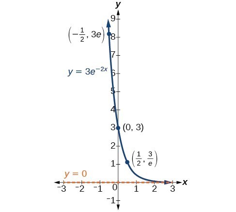
Exponential growth and decay often involve very large or very small numbers. To describe these numbers, we often use orders of magnitude. The order of magnitude is the power of ten, when the number is expressed in scientific notation, with one digit to the left of the decimal. For example, the distance to the nearest star, Proxima Centauri, measured in kilometers, is 40,113,497,200,000 kilometers. Expressed in scientific notation, this is [latex]4.01134972\times {10}^{13}\\[/latex]. So, we could describe this number as having order of magnitude [latex]{10}^{13}\\[/latex].
An exponential function with the form [latex]y={A}_{0}{e}^{kt}\\[/latex] has the following characteristics:
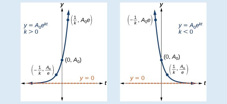
A population of bacteria doubles every hour. If the culture started with 10 bacteria, graph the population as a function of time.
When an amount grows at a fixed percent per unit time, the growth is exponential. To find [latex]{A}_{0}\\[/latex] we use the fact that [latex]{A}_{0}\\[/latex] is the amount at time zero, so [latex]{A}_{0}=10\\[/latex]. To find k, use the fact that after one hour [latex]\left(t=1\right)\\[/latex] the population doubles from 10 to 20. The formula is derived as follows
so [latex]k=\mathrm{ln}\left(2\right)\\[/latex]. Thus the equation we want to graph is [latex]y=10{e}^{\left(\mathrm{ln}2\right)t}=10{\left({e}^{\mathrm{ln}2}\right)}^{t}=10\cdot {2}^{t}\\[/latex]. The graph is shown in Figure 5.
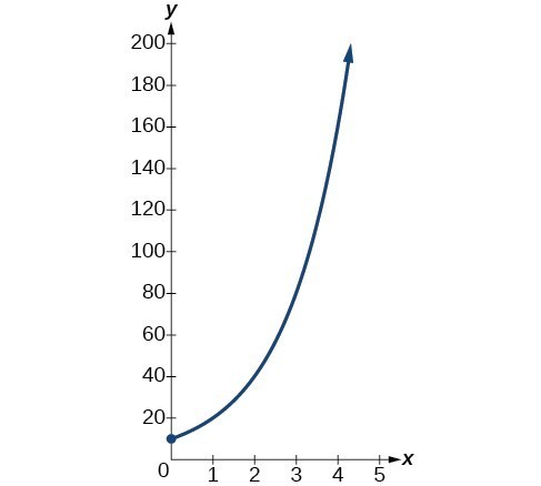
Figure 5. The graph of [latex]y=10{e}^{\left(\mathrm{ln}2\right)t}\\[/latex]
The population of bacteria after ten hours is 10,240. We could describe this amount is being of the order of magnitude [latex]{10}^{4}\\[/latex]. The population of bacteria after twenty hours is 10,485,760 which is of the order of magnitude [latex]{10}^{7}\\[/latex], so we could say that the population has increased by three orders of magnitude in ten hours.
We now turn to exponential decay. One of the common terms associated with exponential decay, as stated above, is half-life, the length of time it takes an exponentially decaying quantity to decrease to half its original amount. Every radioactive isotope has a half-life, and the process describing the exponential decay of an isotope is called radioactive decay.
To find the half-life of a function describing exponential decay, solve the following equation:
We find that the half-life depends only on the constant k and not on the starting quantity [latex]{A}_{0}\\[/latex].
The formula is derived as follows
Since t, the time, is positive, k must, as expected, be negative. This gives us the half-life formula
Note: It is also possible to find the decay rate using [latex]k=-\frac{\mathrm{ln}\left(2\right)}{t}\\[/latex].
The half-life of carbon-14 is 5,730 years. Express the amount of carbon-14 remaining as a function of time, t.
This formula is derived as follows.
The function that describes this continuous decay is [latex]f\left(t\right)={A}_{0}{e}^{\left(\frac{\mathrm{ln}\left(0.5\right)}{5730}\right)t}\\[/latex]. We observe that the coefficient of t, [latex]\frac{\mathrm{ln}\left(0.5\right)}{5730}\approx -1.2097\\[/latex] is negative, as expected in the case of exponential decay.
The half-life of plutonium-244 is 80,000,000 years. Find function gives the amount of carbon-14 remaining as a function of time, measured in years.
The formula for radioactive decay is important in radiocarbon dating, which is used to calculate the approximate date a plant or animal died. Radiocarbon dating was discovered in 1949 by Willard Libby, who won a Nobel Prize for his discovery. It compares the difference between the ratio of two isotopes of carbon in an organic artifact or fossil to the ratio of those two isotopes in the air. It is believed to be accurate to within about 1% error for plants or animals that died within the last 60,000 years.
Carbon-14 is a radioactive isotope of carbon that has a half-life of 5,730 years. It occurs in small quantities in the carbon dioxide in the air we breathe. Most of the carbon on Earth is carbon-12, which has an atomic weight of 12 and is not radioactive. Scientists have determined the ratio of carbon-14 to carbon-12 in the air for the last 60,000 years, using tree rings and other organic samples of known dates—although the ratio has changed slightly over the centuries.
As long as a plant or animal is alive, the ratio of the two isotopes of carbon in its body is close to the ratio in the atmosphere. When it dies, the carbon-14 in its body decays and is not replaced. By comparing the ratio of carbon-14 to carbon-12 in a decaying sample to the known ratio in the atmosphere, the date the plant or animal died can be approximated.
Since the half-life of carbon-14 is 5,730 years, the formula for the amount of carbon-14 remaining after t years is
where
This formula is derived as follows:
To find the age of an object, we solve this equation for t:
Out of necessity, we neglect here the many details that a scientist takes into consideration when doing carbon-14 dating, and we only look at the basic formula. The ratio of carbon-14 to carbon-12 in the atmosphere is approximately 0.0000000001%. Let r be the ratio of carbon-14 to carbon-12 in the organic artifact or fossil to be dated, determined by a method called liquid scintillation. From the equation [latex]A\approx {A}_{0}{e}^{-0.000121t}\\[/latex] we know the ratio of the percentage of carbon-14 in the object we are dating to the percentage of carbon-14 in the atmosphere is [latex]r=\frac{A}{{A}_{0}}\approx {e}^{-0.000121t}\\[/latex]. We solve this equation for t, to get
A bone fragment is found that contains 20% of its original carbon-14. To the nearest year, how old is the bone?
We substitute 20% = 0.20 for k in the equation and solve for t:
The bone fragment is about 13,301 years old.
The instruments that measure the percentage of carbon-14 are extremely sensitive and, as we mention above, a scientist will need to do much more work than we did in order to be satisfied. Even so, carbon dating is only accurate to about 1%, so this age should be given as [latex]\text{13,301 years}\pm \text{1% or 13,301 years}\pm \text{133 years}\\[/latex].
Cesium-137 has a half-life of about 30 years. If we begin with 200 mg of cesium-137, will it take more or less than 230 years until only 1 milligram remains?
For decaying quantities, we determined how long it took for half of a substance to decay. For growing quantities, we might want to find out how long it takes for a quantity to double. As we mentioned above, the time it takes for a quantity to double is called the doubling time.
Given the basic exponential growth equation [latex]A={A}_{0}{e}^{kt}\\[/latex], doubling time can be found by solving for when the original quantity has doubled, that is, by solving [latex]2{A}_{0}={A}_{0}{e}^{kt}\\[/latex].
The formula is derived as follows:
Thus the doubling time is
According to Moore’s Law, the doubling time for the number of transistors that can be put on a computer chip is approximately two years. Give a function that describes this behavior.
The formula is derived as follows:
The function is [latex]A={A}_{0}{e}^{\frac{\mathrm{ln}2}{2}t}\\[/latex].
Recent data suggests that, as of 2013, the rate of growth predicted by Moore’s Law no longer holds. Growth has slowed to a doubling time of approximately three years. Find the new function that takes that longer doubling time into account.
Exponential decay can also be applied to temperature. When a hot object is left in surrounding air that is at a lower temperature, the object’s temperature will decrease exponentially, leveling off as it approaches the surrounding air temperature. On a graph of the temperature function, the leveling off will correspond to a horizontal asymptote at the temperature of the surrounding air. Unless the room temperature is zero, this will correspond to a vertical shift of the generic exponential decay function. This translation leads to Newton’s Law of Cooling, the scientific formula for temperature as a function of time as an object’s temperature is equalized with the ambient temperature
This formula is derived as follows:
The temperature of an object, T, in surrounding air with temperature [latex]{T}_{s}\\[/latex] will behave according to the formula
where
A cheesecake is taken out of the oven with an ideal internal temperature of [latex]165^\circ\text{F}\\[/latex], and is placed into a [latex]35^\circ\text{F}\\[/latex] refrigerator. After 10 minutes, the cheesecake has cooled to [latex]150^\circ\text{F}\\[/latex]. If we must wait until the cheesecake has cooled to [latex]70^\circ\text{F}\\[/latex] before we eat it, how long will we have to wait?
Because the surrounding air temperature in the refrigerator is 35 degrees, the cheesecake’s temperature will decay exponentially toward 35, following the equation
We know the initial temperature was 165, so [latex]T\left(0\right)=165\\[/latex].
We were given another data point, [latex]T\left(10\right)=150\\[/latex], which we can use to solve for k.
This gives us the equation for the cooling of the cheesecake: [latex]T\left(t\right)=130{e}^{-0.0123t}+35\\[/latex].
Now we can solve for the time it will take for the temperature to cool to 70 degrees.
It will take about 107 minutes, or one hour and 47 minutes, for the cheesecake to cool to [latex]70^\circ\text{F}\\[/latex].
A pitcher of water at 40 degrees Fahrenheit is placed into a 70 degree room. One hour later, the temperature has risen to 45 degrees. How long will it take for the temperature to rise to 60 degrees?
Exponential growth cannot continue forever. Exponential models, while they may be useful in the short term, tend to fall apart the longer they continue. Consider an aspiring writer who writes a single line on day one and plans to double the number of lines she writes each day for a month. By the end of the month, she must write over 17 billion lines, or one-half-billion pages. It is impractical, if not impossible, for anyone to write that much in such a short period of time. Eventually, an exponential model must begin to approach some limiting value, and then the growth is forced to slow. For this reason, it is often better to use a model with an upper bound instead of an exponential growth model, though the exponential growth model is still useful over a short term, before approaching the limiting value.
The logistic growth model is approximately exponential at first, but it has a reduced rate of growth as the output approaches the model’s upper bound, called the carrying capacity. For constants a, b, and c, the logistic growth of a population over time x is represented by the model
Figure 6 shows how the growth rate changes over time. The graph increases from left to right, but the growth rate only increases until it reaches its point of maximum growth rate, at which point the rate of increase decreases.
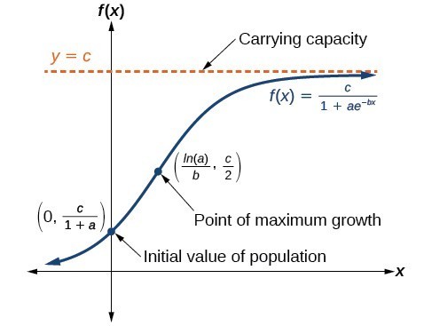
Figure 6
The logistic growth model is
where
An influenza epidemic spreads through a population rapidly, at a rate that depends on two factors: The more people who have the flu, the more rapidly it spreads, and also the more uninfected people there are, the more rapidly it spreads. These two factors make the logistic model a good one to study the spread of communicable diseases. And, clearly, there is a maximum value for the number of people infected: the entire population.
For example, at time t = 0 there is one person in a community of 1,000 people who has the flu. So, in that community, at most 1,000 people can have the flu. Researchers find that for this particular strain of the flu, the logistic growth constant is b = 0.6030. Estimate the number of people in this community who will have had this flu after ten days. Predict how many people in this community will have had this flu after a long period of time has passed.
We substitute the given data into the logistic growth model
Because at most 1,000 people, the entire population of the community, can get the flu, we know the limiting value is c = 1000. To find a, we use the formula that the number of cases at time t = 0 is [latex]\frac{c}{1+a}=1\\[/latex], from which it follows that a = 999. This model predicts that, after ten days, the number of people who have had the flu is [latex]f\left(x\right)=\frac{1000}{1+999{e}^{-0.6030x}}\approx 293.8\\[/latex]. Because the actual number must be a whole number (a person has either had the flu or not) we round to 294. In the long term, the number of people who will contract the flu is the limiting value, c = 1000.
Remember that, because we are dealing with a virus, we cannot predict with certainty the number of people infected. The model only approximates the number of people infected and will not give us exact or actual values.
Figure 7 gives a good picture of how this model fits the data.

Now that we have discussed various mathematical models, we need to learn how to choose the appropriate model for the raw data we have. Many factors influence the choice of a mathematical model, among which are experience, scientific laws, and patterns in the data itself. Not all data can be described by elementary functions. Sometimes, a function is chosen that approximates the data over a given interval. For instance, suppose data were gathered on the number of homes bought in the United States from the years 1960 to 2013. After plotting these data in a scatter plot, we notice that the shape of the data from the years 2000 to 2013 follow a logarithmic curve. We could restrict the interval from 2000 to 2010, apply regression analysis using a logarithmic model, and use it to predict the number of home buyers for the year 2015.
Three kinds of functions that are often useful in mathematical models are linear functions, exponential functions, and logarithmic functions. If the data lies on a straight line, or seems to lie approximately along a straight line, a linear model may be best. If the data is non-linear, we often consider an exponential or logarithmic model, though other models, such as quadratic models, may also be considered.
In choosing between an exponential model and a logarithmic model, we look at the way the data curves. This is called the concavity. If we draw a line between two data points, and all (or most) of the data between those two points lies above that line, we say the curve is concave down. We can think of it as a bowl that bends downward and therefore cannot hold water. If all (or most) of the data between those two points lies below the line, we say the curve is concave up. In this case, we can think of a bowl that bends upward and can therefore hold water. An exponential curve, whether rising or falling, whether representing growth or decay, is always concave up away from its horizontal asymptote. A logarithmic curve is always concave away from its vertical asymptote. In the case of positive data, which is the most common case, an exponential curve is always concave up, and a logarithmic curve always concave down.
A logistic curve changes concavity. It starts out concave up and then changes to concave down beyond a certain point, called a point of inflection.
After using the graph to help us choose a type of function to use as a model, we substitute points, and solve to find the parameters. We reduce round-off error by choosing points as far apart as possible.
Does a linear, exponential, logarithmic, or logistic model best fit the values listed below? Find the model, and use a graph to check your choice.
| x | 1 | 2 | 3 | 4 | 5 | 6 | 7 | 8 | 9 |
| y | 0 | 1.386 | 2.197 | 2.773 | 3.219 | 3.584 | 3.892 | 4.159 | 4.394 |
First, plot the data on a graph as in Figure 8. For the purpose of graphing, round the data to two significant digits.
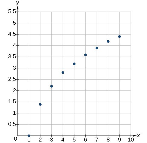
Figure 8
Clearly, the points do not lie on a straight line, so we reject a linear model. If we draw a line between any two of the points, most or all of the points between those two points lie above the line, so the graph is concave down, suggesting a logarithmic model. We can try [latex]y=a\mathrm{ln}\left(bx\right)\\[/latex]. Plugging in the first point, [latex]\left(\text{1,0}\right)\\[/latex], gives [latex]0=a\mathrm{ln}b\\[/latex]. We reject the case that a = 0 (if it were, all outputs would be 0), so we know [latex]\mathrm{ln}\left(b\right)=0\\[/latex]. Thus b = 1 and [latex]y=a\mathrm{ln}\left(\text{x}\right)\\[/latex]. Next we can use the point [latex]\left(\text{9,4}\text{.394}\right)\\[/latex] to solve for a:
Because [latex]a=\frac{4.394}{\mathrm{ln}\left(9\right)}\approx 2\\[/latex], an appropriate model for the data is [latex]y=2\mathrm{ln}\left(x\right)\\[/latex].
To check the accuracy of the model, we graph the function together with the given points.

Figure 9. The graph of [latex]y=2\mathrm{ln}x\\[/latex].
We can conclude that the model is a good fit to the data.
Compare the figure above to the graph of [latex]y=\mathrm{ln}\left({x}^{2}\right)\\[/latex] shown in Figure 10.
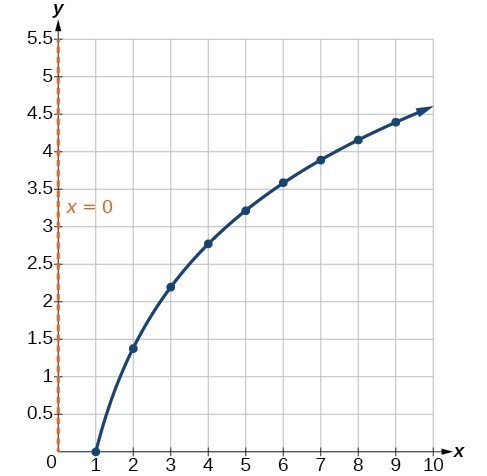
Figure 10. The graph of [latex]y=\mathrm{ln}\left({x}^{2}\right)\\[/latex]
The graphs appear to be identical when x > 0. A quick check confirms this conclusion: [latex]y=\mathrm{ln}\left({x}^{2}\right)=2\mathrm{ln}\left(x\right)\\[/latex] for x > 0.
However, if x < 0, the graph of [latex]y=\mathrm{ln}\left({x}^{2}\right)\\[/latex] includes a “extra” branch, as shown below. This occurs because, while [latex]y=2\mathrm{ln}\left(x\right)\\[/latex] cannot have negative values in the domain (as such values would force the argument to be negative), the function [latex]y=\mathrm{ln}\left({x}^{2}\right)\\[/latex] can have negative domain values.
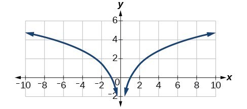
Figure 11
Does a linear, exponential, or logarithmic model best fit the data in the table below? Find the model.
| x | 1 | 2 | 3 | 4 | 5 | 6 | 7 | 8 | 9 |
| y | 3.297 | 5.437 | 8.963 | 14.778 | 24.365 | 40.172 | 66.231 | 109.196 | 180.034 |
While powers and logarithms of any base can be used in modeling, the two most common bases are [latex]10[/latex] and [latex]e[/latex]. In science and mathematics, the base e is often preferred. We can use laws of exponents and laws of logarithms to change any base to base e.
Change the function [latex]y=2.5{\left(3.1\right)}^{x}\\[/latex] so that this same function is written in the form [latex]y={A}_{0}{e}^{kx}\\[/latex].
The formula is derived as follows
Change the function [latex]y=3{\left(0.5\right)}^{x}\\[/latex] to one having e as the base.
| Half-life formula | If [latex]\text{ }A={A}_{0}{e}^{kt}\\[/latex], k < 0, the half-life is [latex]t=-\frac{\mathrm{ln}\left(2\right)}{k}\\[/latex]. |
| Carbon-14 dating | [latex]t=\frac{\mathrm{ln}\left(\frac{A}{{A}_{0}}\right)}{-0.000121}\\[/latex].[latex]{A}_{0}\\[/latex] A is the amount of carbon-14 when the plant or animal died t is the amount of carbon-14 remaining today is the age of the fossil in years |
| Doubling time formula | If [latex]A={A}_{0}{e}^{kt}\\[/latex], k > 0, the doubling time is [latex]t=\frac{\mathrm{ln}2}{k}\\[/latex] |
| Newton’s Law of Cooling | [latex]T\left(t\right)=A{e}^{kt}+{T}_{s}\\[/latex], where [latex]{T}_{s}\\[/latex] is the ambient temperature, [latex]A=T\left(0\right)-{T}_{s}\\[/latex], and k is the continuous rate of cooling. |
1. With what kind of exponential model would half-life be associated? What role does half-life play in these models?
2. What is carbon dating? Why does it work? Give an example in which carbon dating would be useful.
3. With what kind of exponential model would doubling time be associated? What role does doubling time play in these models?
4. Define Newton’s Law of Cooling. Then name at least three real-world situations where Newton’s Law of Cooling would be applied.
5. What is an order of magnitude? Why are orders of magnitude useful? Give an example to explain.
6. The temperature of an object in degrees Fahrenheit after t minutes is represented by the equation [latex]T\left(t\right)=68{e}^{-0.0174t}+72\\[/latex]. To the nearest degree, what is the temperature of the object after one and a half hours?
For the following exercises, use the logistic growth model [latex]f\left(x\right)=\frac{150}{1+8{e}^{-2x}}\\[/latex].
7. Find and interpret [latex]f\left(0\right)\\[/latex]. Round to the nearest tenth.
8. Find and interpret [latex]f\left(4\right)\\[/latex]. Round to the nearest tenth.
9. Find the carrying capacity.
10. Graph the model.
11. Determine whether the data from the table could best be represented as a function that is linear, exponential, or logarithmic. Then write a formula for a model that represents the data.
| x | f (x) |
| –2 | 0.694 |
| –1 | 0.833 |
| 0 | 1 |
| 1 | 1.2 |
| 2 | 1.44 |
| 3 | 1.728 |
| 4 | 2.074 |
| 5 | 2.488 |
12. Rewrite [latex]f\left(x\right)=1.68{\left(0.65\right)}^{x}\\[/latex] as an exponential equation with base e to five significant digits.
For the following exercises, enter the data from each table into a graphing calculator and graph the resulting scatter plots. Determine whether the data from the table could represent a function that is linear, exponential, or logarithmic.
13.
| x | f (x) |
| 1 | 2 |
| 2 | 4.079 |
| 3 | 5.296 |
| 4 | 6.159 |
| 5 | 6.828 |
| 6 | 7.375 |
| 7 | 7.838 |
| 8 | 8.238 |
| 9 | 8.592 |
| 10 | 8.908 |
14.
| x | f(x) |
| 1 | 2.4 |
| 2 | 2.88 |
| 3 | 3.456 |
| 4 | 4.147 |
| 5 | 4.977 |
| 6 | 5.972 |
| 7 | 7.166 |
| 8 | 8.6 |
| 9 | 10.32 |
| 10 | 12.383 |
15.
| x | f(x) |
| 4 | 9.429 |
| 5 | 9.972 |
| 6 | 10.415 |
| 7 | 10.79 |
| 8 | 11.115 |
| 9 | 11.401 |
| 10 | 11.657 |
| 11 | 11.889 |
| 12 | 12.101 |
| 13 | 12.295 |
16.
| x | f(x) |
| 1.25 | 5.75 |
| 2.25 | 8.75 |
| 3.56 | 12.68 |
| 4.2 | 14.6 |
| 5.65 | 18.95 |
| 6.75 | 22.25 |
| 7.25 | 23.75 |
| 8.6 | 27.8 |
| 9.25 | 29.75 |
| 10.5 | 33.5 |
For the following exercises, use a graphing calculator and this scenario: the population of a fish farm in t years is modeled by the equation [latex]P\left(t\right)=\frac{1000}{1+9{e}^{-0.6t}}\\[/latex].
17. Graph the function.
18. What is the initial population of fish?
19. To the nearest tenth, what is the doubling time for the fish population?
20. To the nearest whole number, what will the fish population be after 2 years?
21. To the nearest tenth, how long will it take for the population to reach 900?
22. What is the carrying capacity for the fish population? Justify your answer using the graph of P.
23. A substance has a half-life of 2.045 minutes. If the initial amount of the substance was 132.8 grams, how many half-lives will have passed before the substance decays to 8.3 grams? What is the total time of decay?
24. The formula for an increasing population is given by [latex]P\left(t\right)={P}_{0}{e}^{rt}\\[/latex] where [latex]{P}_{0}\\[/latex] is the initial population and r > 0. Derive a general formula for the time t it takes for the population to increase by a factor of M.
25. Recall the formula for calculating the magnitude of an earthquake, [latex]M=\frac{2}{3}\mathrm{log}\left(\frac{S}{{S}_{0}}\right)\\[/latex]. Show each step for solving this equation algebraically for the seismic moment S.
26. What is the y-intercept of the logistic growth model [latex]y=\frac{c}{1+a{e}^{-rx}}\\[/latex]? Show the steps for calculation. What does this point tell us about the population?
27. Prove that [latex]{b}^{x}={e}^{x\mathrm{ln}\left(b\right)}\\[/latex] for positive [latex]b\ne 1\\[/latex].
For the following exercises, use this scenario: A doctor prescribes 125 milligrams of a therapeutic drug that decays by about 30% each hour.
28. To the nearest hour, what is the half-life of the drug?
29. Write an exponential model representing the amount of the drug remaining in the patient’s system after t hours. Then use the formula to find the amount of the drug that would remain in the patient’s system after 3 hours. Round to the nearest milligram.
30. Using the model found in the previous exercise, find [latex]f\left(10\right)\\[/latex] and interpret the result. Round to the nearest hundredth.
For the following exercises, use this scenario: A tumor is injected with 0.5 grams of Iodine-125, which has a decay rate of 1.15% per day.
31. To the nearest day, how long will it take for half of the Iodine-125 to decay?
32. Write an exponential model representing the amount of Iodine-125 remaining in the tumor after t days. Then use the formula to find the amount of Iodine-125 that would remain in the tumor after 60 days. Round to the nearest tenth of a gram.
33. A scientist begins with 250 grams of a radioactive substance. After 250 minutes, the sample has decayed to 32 grams. Rounding to five significant digits, write an exponential equation representing this situation. To the nearest minute, what is the half-life of this substance?
34. The half-life of Radium-226 is 1590 years. What is the annual decay rate? Express the decimal result to four significant digits and the percentage to two significant digits.
35. The half-life of Erbium-165 is 10.4 hours. What is the hourly decay rate? Express the decimal result to four significant digits and the percentage to two significant digits.
36. A wooden artifact from an archeological dig contains 60 percent of the carbon-14 that is present in living trees. To the nearest year, about how many years old is the artifact? (The half-life of carbon-14 is 5730 years.)
37. A research student is working with a culture of bacteria that doubles in size every twenty minutes. The initial population count was 1350 bacteria. Rounding to five significant digits, write an exponential equation representing this situation. To the nearest whole number, what is the population size after 3 hours?
For the following exercises, use this scenario: A biologist recorded a count of 360 bacteria present in a culture after 5 minutes and 1000 bacteria present after 20 minutes.
38. To the nearest whole number, what was the initial population in the culture?
39. Rounding to six significant digits, write an exponential equation representing this situation. To the nearest minute, how long did it take the population to double?
For the following exercises, use this scenario: A pot of boiling soup with an internal temperature of 100º Fahrenheit was taken off the stove to cool in a 69ºF room. After fifteen minutes, the internal temperature of the soup was 95ºF.
40. Use Newton’s Law of Cooling to write a formula that models this situation.
41. To the nearest minute, how long will it take the soup to cool to 80ºF?
42. To the nearest degree, what will the temperature be after 2 and a half hours?
For the following exercises, use this scenario: A turkey is taken out of the oven with an internal temperature of 165ºF and is allowed to cool in a 75ºF room. After half an hour, the internal temperature of the turkey is 145ºF.
43. Write a formula that models this situation.
44. To the nearest degree, what will the temperature be after 50 minutes?
45. To the nearest minute, how long will it take the turkey to cool to 110ºF?
For the following exercises, find the value of the number shown on each logarithmic scale. Round all answers to the nearest thousandth.
46.
47.
48. Plot each set of approximate values of intensity of sounds on a logarithmic scale: Whisper: [latex]{10}^{-10} \frac{W}{{m}^{2}}\\[/latex], Vacuum: [latex]{10}^{-4}\frac{W}{{m}^{2}}\\[/latex], Jet: [latex]{10}^{2} \frac{W}{{m}^{2}}\\[/latex]
49. Recall the formula for calculating the magnitude of an earthquake, [latex]M=\frac{2}{3}\mathrm{log}\left(\frac{S}{{S}_{0}}\right)\\[/latex]. One earthquake has magnitude 3.9 on the MMS scale. If a second earthquake has 750 times as much energy as the first, find the magnitude of the second quake. Round to the nearest hundredth.
For the following exercises, use this scenario: The equation [latex]N\left(t\right)=\frac{500}{1+49{e}^{-0.7t}}\\[/latex] models the number of people in a town who have heard a rumor after t days.
50. How many people started the rumor?
51. To the nearest whole number, how many people will have heard the rumor after 3 days?
52. As t increases without bound, what value does N(t) approach? Interpret your answer.
For the following exercise, choose the correct answer choice.
53. A doctor and injects a patient with 13 milligrams of radioactive dye that decays exponentially. After 12 minutes, there are 4.75 milligrams of dye remaining in the patient’s system. Which is an appropriate model for this situation?
A. [latex]f\left(t\right)=13{\left(0.0805\right)}^{t}\\[/latex]
B. [latex]f\left(t\right)=13{e}^{0.9195t}\\[/latex]
C. [latex]f\left(t\right)=13{e}^{\left(-0.0839t\right)}\\[/latex]
D. [latex]f\left(t\right)=\frac{4.75}{1+13{e}^{-0.83925t}}\\[/latex]
1. [latex]f\left(t\right)={A}_{0}{e}^{-0.0000000087t}\\[/latex]
2. less than 230 years, 229.3157 to be exact
3. [latex]f\left(t\right)={A}_{0}{e}^{\frac{\mathrm{ln}2}{3}t}\\[/latex]
4. 6.026 hours
5. 895 cases on day 15
6. Exponential. [latex]y=2{e}^{0.5x}\\[/latex].
7. [latex]y=3{e}^{\left(\mathrm{ln}0.5\right)x}\\[/latex]
1. Half-life is a measure of decay and is thus associated with exponential decay models. The half-life of a substance or quantity is the amount of time it takes for half of the initial amount of that substance or quantity to decay.
3. Doubling time is a measure of growth and is thus associated with exponential growth models. The doubling time of a substance or quantity is the amount of time it takes for the initial amount of that substance or quantity to double in size.
5. An order of magnitude is the nearest power of ten by which a quantity exponentially grows. It is also an approximate position on a logarithmic scale; Sample response: Orders of magnitude are useful when making comparisons between numbers that differ by a great amount. For example, the mass of Saturn is 95 times greater than the mass of Earth. This is the same as saying that the mass of Saturn is about [latex]{10}^{\text{2}}\\[/latex] times, or 2 orders of magnitude greater, than the mass of Earth.
7. [latex]f\left(0\right)\approx 16.7\\[/latex]; The amount initially present is about 16.7 units.
9. 150
11. exponential; [latex]f\left(x\right)={1.2}^{x}\\[/latex]
13. logarithmic
15. logarithmic
17.
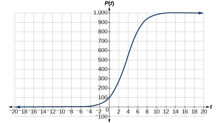
19. about 1.4 years
21. about 7.3 years
23. 4 half-lives; 8.18 minutes
25. [latex]\begin{cases}\text{ }M=\frac{2}{3}\mathrm{log}\left(\frac{S}{{S}_{0}}\right)\hfill \\ \mathrm{log}\left(\frac{S}{{S}_{0}}\right)=\frac{3}{2}M\hfill \\ \text{ }\frac{S}{{S}_{0}}={10}^{\frac{3M}{2}}\hfill \\ \text{ }S={S}_{0}{10}^{\frac{3M}{2}}\hfill \end{cases}//[/latex]
27. Let [latex]y={b}^{x}\\[/latex] for some non-negative real number b such that [latex]b\ne 1\\[/latex]. Then,
[latex]\begin{cases}\mathrm{ln}\left(y\right)=\mathrm{ln}\left({b}^{x}\right)\hfill \\ \mathrm{ln}\left(y\right)=x\mathrm{ln}\left(b\right)\hfill \\ {e}^{\mathrm{ln}\left(y\right)}={e}^{x\mathrm{ln}\left(b\right)}\hfill \\ y={e}^{x\mathrm{ln}\left(b\right)}\hfill \end{cases}\\[/latex]
29. [latex]A=125{e}^{\left(-0.3567t\right)};A\approx 43\\[/latex] mg
31. about 60 days
33. [latex]f\left(t\right)=250{e}^{\left(-0.00914t\right)}\\[/latex]; half-life: about [latex]\text{76}\\[/latex] minutes
35. [latex]r\approx -0.0667\\[/latex], So the hourly decay rate is about 6.67%
37. [latex]f\left(t\right)=1350{e}^{\left(0.03466t\right)}\\[/latex]; after 3 hours: [latex]P\left(180\right)\approx 691,200\\[/latex]
39. [latex]f\left(t\right)=256{e}^{\left(0.068110t\right)}\\[/latex]; doubling time: about 10 minutes
41. about 88 minutes
43. [latex]T\left(t\right)=90{e}^{\left(-0.008377t\right)}+75\\[/latex], where t is in minutes.
45. about 113 minutes
47. [latex]\mathrm{log}\left(x\right)=1.5;x\approx 31.623\\[/latex]
49. MMS magnitude: 5.82
51. [latex]N\left(3\right)\approx 71\\[/latex]
53. C
By the end of this section, you will be able to:
Figure 1. (credit: Thomas Sørenes)
A skateboard manufacturer introduces a new line of boards. The manufacturer tracks its costs, which is the amount it spends to produce the boards, and its revenue, which is the amount it earns through sales of its boards. How can the company determine if it is making a profit with its new line? How many skateboards must be produced and sold before a profit is possible? In this section, we will consider linear equations with two variables to answer these and similar questions.
In order to investigate situations such as that of the skateboard manufacturer, we need to recognize that we are dealing with more than one variable and likely more than one equation. A system of linear equations consists of two or more linear equations made up of two or more variables such that all equations in the system are considered simultaneously. To find the unique solution to a system of linear equations, we must find a numerical value for each variable in the system that will satisfy all equations in the system at the same time. Some linear systems may not have a solution and others may have an infinite number of solutions. In order for a linear system to have a unique solution, there must be at least as many equations as there are variables. Even so, this does not guarantee a unique solution.
In this section, we will look at systems of linear equations in two variables, which consist of two equations that contain two different variables. For example, consider the following system of linear equations in two variables.
The solution to a system of linear equations in two variables is any ordered pair that satisfies each equation independently. In this example, the ordered pair (4, 7) is the solution to the system of linear equations. We can verify the solution by substituting the values into each equation to see if the ordered pair satisfies both equations. Shortly we will investigate methods of finding such a solution if it exists.
In addition to considering the number of equations and variables, we can categorize systems of linear equations by the number of solutions. A consistent system of equations has at least one solution. A consistent system is considered to be an independent system if it has a single solution, such as the example we just explored. The two lines have different slopes and intersect at one point in the plane. A consistent system is considered to be a dependent system if the equations have the same slope and the same y-intercepts. In other words, the lines coincide so the equations represent the same line. Every point on the line represents a coordinate pair that satisfies the system. Thus, there are an infinite number of solutions.
Another type of system of linear equations is an inconsistent system, which is one in which the equations represent two parallel lines. The lines have the same slope and different y-intercepts. There are no points common to both lines; hence, there is no solution to the system.
There are three types of systems of linear equations in two variables, and three types of solutions.
Figure 2 compares graphical representations of each type of system.
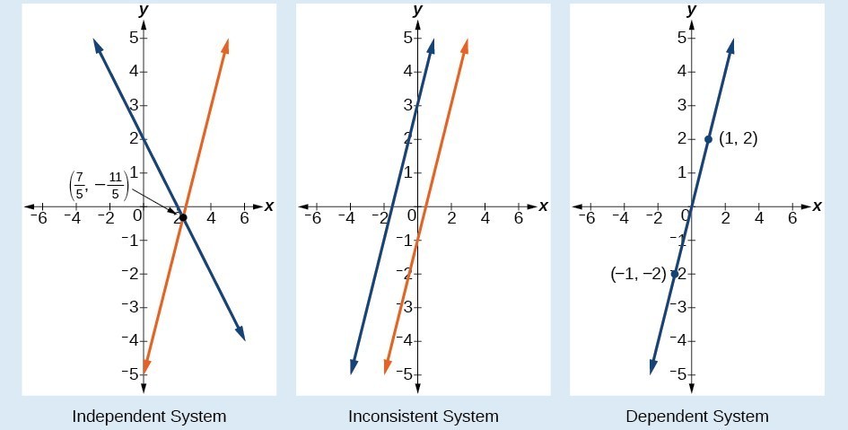
Figure 2
Determine whether the ordered pair [latex]\left(5,1\right)[/latex] is a solution to the given system of equations.
Substitute the ordered pair [latex]\left(5,1\right)[/latex] into both equations.
The ordered pair [latex]\left(5,1\right)[/latex] satisfies both equations, so it is the solution to the system.
We can see the solution clearly by plotting the graph of each equation. Since the solution is an ordered pair that satisfies both equations, it is a point on both of the lines and thus the point of intersection of the two lines.
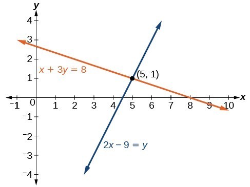
Figure 3
Determine whether the ordered pair [latex]\left(8,5\right)[/latex] is a solution to the following system.
There are multiple methods of solving systems of linear equations. For a system of linear equations in two variables, we can determine both the type of system and the solution by graphing the system of equations on the same set of axes.
Solve the following system of equations by graphing. Identify the type of system.
Solve the first equation for [latex]y[/latex].
Solve the second equation for [latex]y[/latex].
Graph both equations on the same set of axes as in Figure 4.
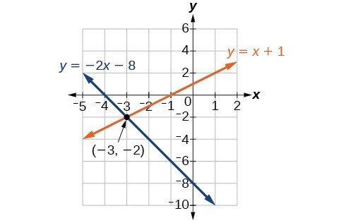
Figure 4
The lines appear to intersect at the point [latex]\left(-3,-2\right)[/latex]. We can check to make sure that this is the solution to the system by substituting the ordered pair into both equations.
The solution to the system is the ordered pair [latex]\left(-3,-2\right)[/latex], so the system is independent.
Solve the following system of equations by graphing.
Yes, in both cases we can still graph the system to determine the type of system and solution. If the two lines are parallel, the system has no solution and is inconsistent. If the two lines are identical, the system has infinite solutions and is a dependent system.
Solving a linear system in two variables by graphing works well when the solution consists of integer values, but if our solution contains decimals or fractions, it is not the most precise method. We will consider two more methods of solving a system of linear equations that are more precise than graphing. One such method is solving a system of equations by the substitution method, in which we solve one of the equations for one variable and then substitute the result into the second equation to solve for the second variable. Recall that we can solve for only one variable at a time, which is the reason the substitution method is both valuable and practical.
Solve the following system of equations by substitution.
First, we will solve the first equation for [latex]y[/latex].
Now we can substitute the expression [latex]x - 5[/latex] for [latex]y[/latex] in the second equation.
Now, we substitute [latex]x=8[/latex] into the first equation and solve for [latex]y[/latex].
Our solution is [latex]\left(8,3\right)[/latex].
Check the solution by substituting [latex]\left(8,3\right)[/latex] into both equations.
Solve the following system of equations by substitution.
Yes, but the method works best if one of the equations contains a coefficient of 1 or –1 so that we do not have to deal with fractions.
A third method of solving systems of linear equations is the addition method. In this method, we add two terms with the same variable, but opposite coefficients, so that the sum is zero. Of course, not all systems are set up with the two terms of one variable having opposite coefficients. Often we must adjust one or both of the equations by multiplication so that one variable will be eliminated by addition.
Solve the given system of equations by addition.
Both equations are already set equal to a constant. Notice that the coefficient of [latex]x[/latex] in the second equation, –1, is the opposite of the coefficient of [latex]x[/latex] in the first equation, 1. We can add the two equations to eliminate [latex]x[/latex] without needing to multiply by a constant.
Now that we have eliminated [latex]x[/latex], we can solve the resulting equation for [latex]y[/latex].
Then, we substitute this value for [latex]y[/latex] into one of the original equations and solve for [latex]x[/latex].
The solution to this system is [latex]\left(-\frac{7}{3},\frac{2}{3}\right)[/latex].
Check the solution in the first equation.
We gain an important perspective on systems of equations by looking at the graphical representation. See Figure 5 to find that the equations intersect at the solution. We do not need to ask whether there may be a second solution because observing the graph confirms that the system has exactly one solution.
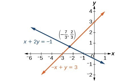
Figure 5
Solve the given system of equations by the addition method.
Adding these equations as presented will not eliminate a variable. However, we see that the first equation has [latex]3x[/latex] in it and the second equation has [latex]x[/latex]. So if we multiply the second equation by [latex]-3,\text{}[/latex] the x-terms will add to zero.
Now, let’s add them.
[latex]\begin{array}\ \hfill 3x+5y=−11 \\ \hfill −3x+6y=−33 \\ \text{_____________} \\ \hfill 11y=−44 \\ \hfill y=−4 \end{array}[/latex]
For the last step, we substitute [latex]y=-4[/latex] into one of the original equations and solve for [latex]x[/latex].
Our solution is the ordered pair [latex]\left(3,-4\right)[/latex]. Check the solution in the original second equation.
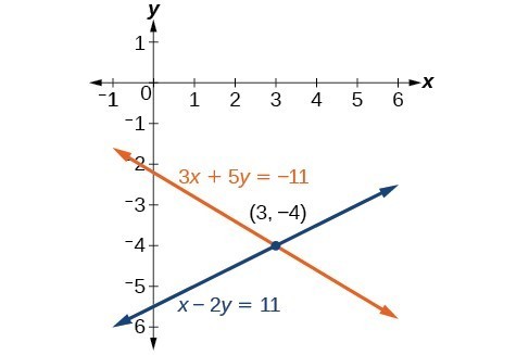
Figure 6
Solve the system of equations by addition.
Solve the given system of equations in two variables by addition.
One equation has [latex]2x[/latex] and the other has [latex]5x[/latex]. The least common multiple is [latex]10x[/latex] so we will have to multiply both equations by a constant in order to eliminate one variable. Let’s eliminate [latex]x[/latex] by multiplying the first equation by [latex]-5[/latex] and the second equation by [latex]2[/latex].
Then, we add the two equations together.
[latex]\begin{array}\ −10x−15y=80 \\ 10x−20y=60 \\ \text{______________} \\ \text{ }−35y=140 \\ y=−4 \end{array}[/latex]
Substitute [latex]y=-4[/latex] into the original first equation.
The solution is [latex]\left(-2,-4\right)[/latex]. Check it in the other equation.
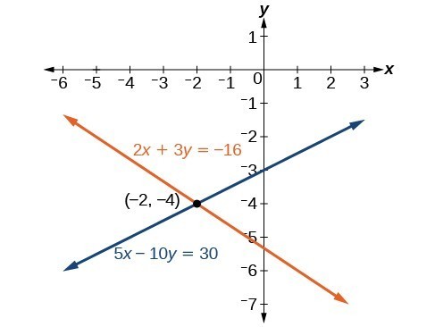
Figure 7
Solve the given system of equations in two variables by addition.
First clear each equation of fractions by multiplying both sides of the equation by the least common denominator.
Now multiply the second equation by [latex]-1[/latex] so that we can eliminate the x-variable.
Add the two equations to eliminate the x-variable and solve the resulting equation.
[latex]\begin{array}\ \hfill 2x+y=18 \\ \hfill−2x+y=−4 \\ \text{_____________} \\ \hfill 2y=14 \\ \hfill y=7 \end{array}[/latex]
Substitute [latex]y=7[/latex] into the first equation.
The solution is [latex]\left(\frac{11}{2},7\right)[/latex]. Check it in the other equation.
Solve the system of equations by addition.
Now that we have several methods for solving systems of equations, we can use the methods to identify inconsistent systems. Recall that an inconsistent system consists of parallel lines that have the same slope but different [latex]y[/latex] -intercepts. They will never intersect. When searching for a solution to an inconsistent system, we will come up with a false statement, such as [latex]12=0[/latex].
Solve the following system of equations.
We can approach this problem in two ways. Because one equation is already solved for [latex]x[/latex], the most obvious step is to use substitution.
Clearly, this statement is a contradiction because [latex]9\ne 13[/latex]. Therefore, the system has no solution.
The second approach would be to first manipulate the equations so that they are both in slope-intercept form. We manipulate the first equation as follows.
We then convert the second equation expressed to slope-intercept form.
Comparing the equations, we see that they have the same slope but different y-intercepts. Therefore, the lines are parallel and do not intersect.
Writing the equations in slope-intercept form confirms that the system is inconsistent because all lines will intersect eventually unless they are parallel. Parallel lines will never intersect; thus, the two lines have no points in common. The graphs of the equations in this example are shown in Figure 8.
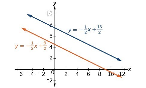
Figure 8
Solve the following system of equations in two variables.
Recall that a dependent system of equations in two variables is a system in which the two equations represent the same line. Dependent systems have an infinite number of solutions because all of the points on one line are also on the other line. After using substitution or addition, the resulting equation will be an identity, such as [latex]0=0[/latex].
Find a solution to the system of equations using the addition method.
With the addition method, we want to eliminate one of the variables by adding the equations. In this case, let’s focus on eliminating [latex]x[/latex]. If we multiply both sides of the first equation by [latex]-3[/latex], then we will be able to eliminate the [latex]x[/latex] -variable.
Now add the equations.
[latex]\begin{array} \hfill−3x−9y=−6 \\ \hfill+3x+9y=6 \\ \hfill \text{_____________} \\ \hfill 0=0 \end{array}[/latex]
We can see that there will be an infinite number of solutions that satisfy both equations.
If we rewrote both equations in the slope-intercept form, we might know what the solution would look like before adding. Let’s look at what happens when we convert the system to slope-intercept form.
See Figure 9. Notice the results are the same. The general solution to the system is [latex]\left(x, -\frac{1}{3}x+\frac{2}{3}\right)[/latex].
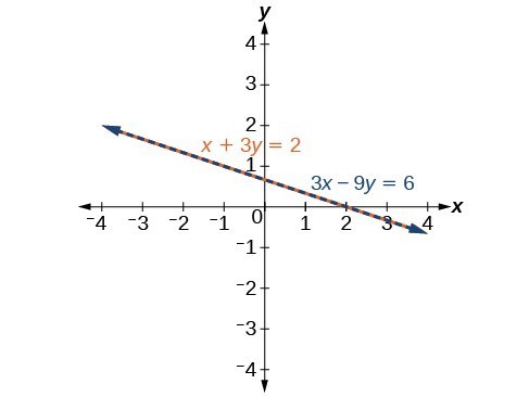
Figure 9
Solve the following system of equations in two variables.
Using what we have learned about systems of equations, we can return to the skateboard manufacturing problem at the beginning of the section. The skateboard manufacturer’s revenue function is the function used to calculate the amount of money that comes into the business. It can be represented by the equation [latex]R=xp[/latex], where [latex]x=[/latex] quantity and [latex]p=[/latex] price. The revenue function is shown in orange in Figure 10.
The cost function is the function used to calculate the costs of doing business. It includes fixed costs, such as rent and salaries, and variable costs, such as utilities. The cost function is shown in blue in Figure 10. The [latex]x[/latex] -axis represents quantity in hundreds of units. The y-axis represents either cost or revenue in hundreds of dollars.
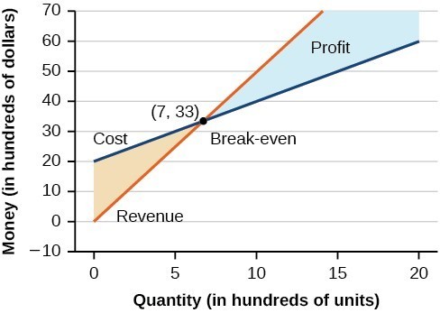
The point at which the two lines intersect is called the break-even point. We can see from the graph that if 700 units are produced, the cost is $3,300 and the revenue is also $3,300. In other words, the company breaks even if they produce and sell 700 units. They neither make money nor lose money.
The shaded region to the right of the break-even point represents quantities for which the company makes a profit. The shaded region to the left represents quantities for which the company suffers a loss. The profit function is the revenue function minus the cost function, written as [latex]P\left(x\right)=R\left(x\right)-C\left(x\right)[/latex]. Clearly, knowing the quantity for which the cost equals the revenue is of great importance to businesses.
Given the cost function [latex]C\left(x\right)=0.85x+35,000[/latex] and the revenue function [latex]R\left(x\right)=1.55x[/latex], find the break-even point and the profit function.
Write the system of equations using [latex]y[/latex] to replace function notation.
Substitute the expression [latex]0.85x+35,000[/latex] from the first equation into the second equation and solve for [latex]x[/latex].
Then, we substitute [latex]x=50,000[/latex] into either the cost function or the revenue function.
The break-even point is [latex]\left(50,000,77,500\right)[/latex].
The profit function is found using the formula [latex]P\left(x\right)=R\left(x\right)-C\left(x\right)[/latex].
The profit function is [latex]P\left(x\right)=0.7x - 35,000[/latex].
The cost to produce 50,000 units is $77,500, and the revenue from the sales of 50,000 units is also $77,500. To make a profit, the business must produce and sell more than 50,000 units.
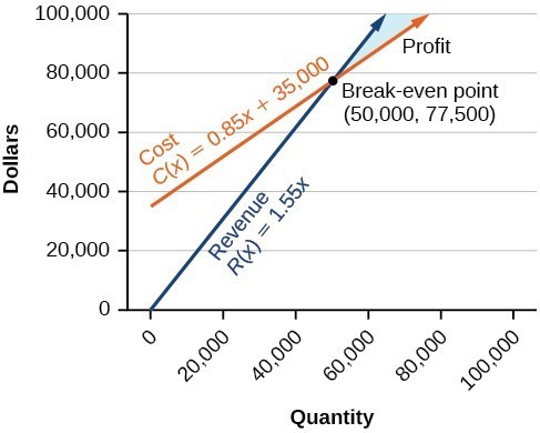
Figure 11
We see from the graph in Figure 12 that the profit function has a negative value until [latex]x=50,000[/latex], when the graph crosses the x-axis. Then, the graph emerges into positive y-values and continues on this path as the profit function is a straight line. This illustrates that the break-even point for businesses occurs when the profit function is 0. The area to the left of the break-even point represents operating at a loss.
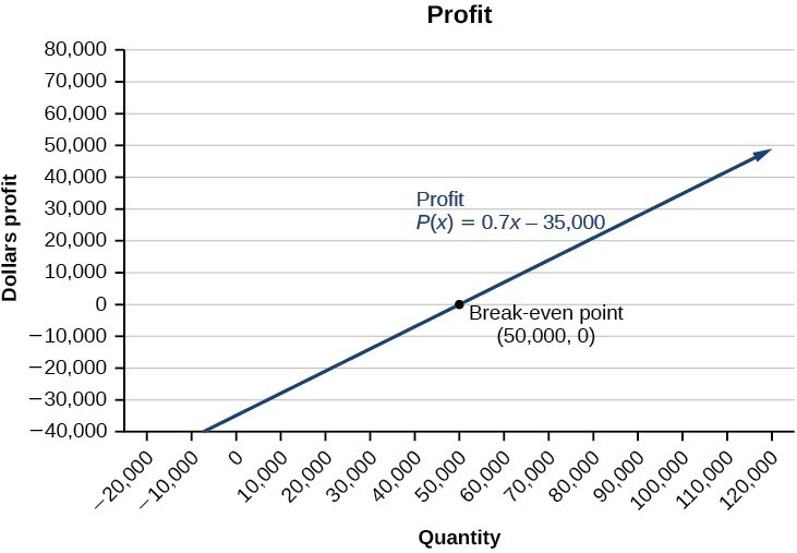
Figure 12
The cost of a ticket to the circus is $25.00 for children and $50.00 for adults. On a certain day, attendance at the circus is 2,000 and the total gate revenue is $70,000. How many children and how many adults bought tickets?
Let c = the number of children and a = the number of adults in attendance.
The total number of people is [latex]2,000[/latex]. We can use this to write an equation for the number of people at the circus that day.
The revenue from all children can be found by multiplying $25.00 by the number of children, [latex]25c[/latex]. The revenue from all adults can be found by multiplying $50.00 by the number of adults, [latex]50a[/latex]. The total revenue is $70,000. We can use this to write an equation for the revenue.
We now have a system of linear equations in two variables.
In the first equation, the coefficient of both variables is 1. We can quickly solve the first equation for either [latex]c[/latex] or [latex]a[/latex]. We will solve for [latex]a[/latex].
Substitute the expression [latex]2,000-c[/latex] in the second equation for [latex]a[/latex] and solve for [latex]c[/latex].
Substitute [latex]c=1,200[/latex] into the first equation to solve for [latex]a[/latex].
We find that [latex]1,200[/latex] children and [latex]800[/latex] adults bought tickets to the circus that day.
Meal tickets at the circus cost $4.00 for children and $12.00 for adults. If 1,650 meal tickets were bought for a total of $14,200, how many children and how many adults bought meal tickets?
1. Can a system of linear equations have exactly two solutions? Explain why or why not.
2. If you are performing a break-even analysis for a business and their cost and revenue equations are dependent, explain what this means for the company’s profit margins.
3. If you are solving a break-even analysis and get a negative break-even point, explain what this signifies for the company?
4. If you are solving a break-even analysis and there is no break-even point, explain what this means for the company. How should they ensure there is a break-even point?
5. Given a system of equations, explain at least two different methods of solving that system.
For the following exercises, determine whether the given ordered pair is a solution to the system of equations.
6. [latex]\begin{array}{c}5x-y=4\\ x+6y=2\end{array}[/latex] and [latex]\left(4,0\right)[/latex]
7. [latex]\begin{array}{l}-3x - 5y=13\hfill \\ -x+4y=10\hfill \end{array}[/latex] and [latex]\left(-6,1\right)[/latex]
8. [latex]\begin{array}{c}3x+7y=1\\ 2x+4y=0\end{array}[/latex] and [latex]\left(2,3\right)[/latex]
9. [latex]\begin{array}{l}-2x+5y=7\hfill \\ \text{ }2x+9y=7\hfill \end{array}[/latex] and [latex]\left(-1,1\right)[/latex]
10. [latex]\begin{array}{c}x+8y=43\\ 3x - 2y=-1\end{array}[/latex] and [latex]\left(3,5\right)[/latex]
For the following exercises, solve each system by substitution.
11. [latex]\begin{array}{l}\text{ }x+3y=5\hfill \\ 2x+3y=4\hfill \end{array}[/latex]
12. [latex]\begin{array}{l}\text{ }3x - 2y=18\hfill \\ 5x+10y=-10\hfill \end{array}[/latex]
13. [latex]\begin{array}{l}4x+2y=-10\\ 3x+9y=0\end{array}[/latex]
14. [latex]\begin{array}{l}2x+4y=-3.8\\ 9x - 5y=1.3\end{array}[/latex]
15. [latex]\begin{array}{l}\hfill \\ \begin{array}{l}\\ \begin{array}{l}-2x+3y=1.2\hfill \\ -3x - 6y=1.8\hfill \end{array}\end{array}\hfill \end{array}[/latex]
16. [latex]\begin{array}{l}\text{ }x - 0.2y=1\hfill \\ -10x+2y=5\hfill \end{array}[/latex]
17. [latex]\begin{array}{l}\text{ }3x+5y=9\hfill \\ 30x+50y=-90\hfill \end{array}[/latex]
18. [latex]\begin{array}{l}\hfill \\ \begin{array}{l}\text{ }-3x+y=2\hfill \\ 12x - 4y=-8\hfill \end{array}\hfill \end{array}[/latex]
19. [latex]\begin{array}{l}\frac{1}{2}x+\frac{1}{3}y=16\\ \frac{1}{6}x+\frac{1}{4}y=9\end{array}[/latex]
20. [latex]\begin{array}{l}\\ \begin{array}{l}-\frac{1}{4}x+\frac{3}{2}y=11\hfill \\ -\frac{1}{8}x+\frac{1}{3}y=3\hfill \end{array}\end{array}[/latex]
For the following exercises, solve each system by addition.
21. [latex]\begin{array}{l}\hfill \\ \begin{array}{l}-2x+5y=-42\hfill \\ \text{ }7x+2y=30\hfill \end{array}\hfill \end{array}[/latex]
22. [latex]\begin{array}{l}6x - 5y=-34\\ 2x+6y=4\end{array}[/latex]
23. [latex]\begin{array}{l}\text{ }5x-y=-2.6\hfill \\ -4x - 6y=1.4\hfill \end{array}[/latex]
24. [latex]\begin{array}{l}7x - 2y=3\\ 4x+5y=3.25\end{array}[/latex]
25. [latex]\begin{array}{l}\hfill \\ \begin{array}{l}\text{ }\mathrm{-x}+2y=-1\hfill \\ 5x - 10y=6\hfill \end{array}\hfill \end{array}[/latex]
26. [latex]\begin{array}{l}\text{ }7x+6y=2\hfill \\ -28x - 24y=-8\hfill \end{array}[/latex]
27. [latex]\begin{array}{l}\frac{5}{6}x+\frac{1}{4}y=0\\ \frac{1}{8}x-\frac{1}{2}y=-\frac{43}{120}\end{array}[/latex]
28. [latex]\begin{array}{l}\text{ }\frac{1}{3}x+\frac{1}{9}y=\frac{2}{9}\hfill \\ -\frac{1}{2}x+\frac{4}{5}y=-\frac{1}{3}\hfill \end{array}[/latex]
29. [latex]\begin{array}{l}\hfill \\ \begin{array}{l}-0.2x+0.4y=0.6\hfill \\ \text{ }x - 2y=-3\hfill \end{array}\hfill \end{array}[/latex]
30. [latex]\begin{array}{l}\begin{array}{l}\\ -0.1x+0.2y=0.6\end{array}\hfill \\ \text{ }5x - 10y=1\hfill \end{array}[/latex]
For the following exercises, solve each system by any method.
31. [latex]\begin{array}{l}5x+9y=16\hfill \\ \text{ }x+2y=4\hfill \end{array}[/latex]
32. [latex]\begin{array}{l}6x - 8y=-0.6\\ 3x+2y=0.9\end{array}[/latex]
33. [latex]\begin{array}{l}5x - 2y=2.25\\ 7x - 4y=3\end{array}[/latex]
34. [latex]\begin{array}{l}\begin{array}{l}\hfill \\ \text{ }x-\frac{5}{12}y=-\frac{55}{12}\hfill \end{array}\hfill \\ -6x+\frac{5}{2}y=\frac{55}{2}\hfill \end{array}[/latex]
35. [latex]\begin{array}{l}\\ \begin{array}{l}7x - 4y=\frac{7}{6}\hfill \\ 2x+4y=\frac{1}{3}\hfill \end{array}\end{array}[/latex]
36. [latex]\begin{array}{l}3x+6y=11\\ 2x+4y=9\end{array}[/latex]
37. [latex]\begin{array}{l}\text{ }\frac{7}{3}x-\frac{1}{6}y=2\hfill \\ -\frac{21}{6}x+\frac{3}{12}y=-3\hfill \end{array}[/latex]
38. [latex]\begin{array}{l}\frac{1}{2}x+\frac{1}{3}y=\frac{1}{3}\\ \frac{3}{2}x+\frac{1}{4}y=-\frac{1}{8}\end{array}[/latex]
39. [latex]\begin{array}{l}2.2x+1.3y=-0.1\\ 4.2x+4.2y=2.1\end{array}[/latex]
40. [latex]\begin{array}{l}\text{ }0.1x+0.2y=2\hfill \\ 0.35x - 0.3y=0\hfill \end{array}[/latex]
For the following exercises, graph the system of equations and state whether the system is consistent, inconsistent, or dependent and whether the system has one solution, no solution, or infinite solutions.
41. [latex]\begin{array}{l}3x-y=0.6\\ x - 2y=1.3\end{array}[/latex]
42. [latex]\begin{array}{l}\begin{array}{l}\\ -x+2y=4\end{array}\hfill \\ \text{ }2x - 4y=1\hfill \end{array}[/latex]
43. [latex]\begin{array}{l}\text{ }x+2y=7\hfill \\ 2x+6y=12\hfill \end{array}[/latex]
44. [latex]\begin{array}{l}3x - 5y=7\hfill \\ \text{ }x - 2y=3\hfill \end{array}[/latex]
45. [latex]\begin{array}{l}\text{ }3x - 2y=5\hfill \\ -9x+6y=-15\hfill \end{array}[/latex]
For the following exercises, use the intersect function on a graphing device to solve each system. Round all answers to the nearest hundredth.
46. [latex]\begin{array}{l}\text{ }0.1x+0.2y=0.3\hfill \\ -0.3x+0.5y=1\hfill \end{array}[/latex]
47. [latex]\begin{array}{l}\hfill \\ \begin{array}{l}-0.01x+0.12y=0.62\hfill \\ 0.15x+0.20y=0.52\hfill \end{array}\hfill \end{array}[/latex]
48. [latex]\begin{array}{l}0.5x+0.3y=4\hfill \\ 0.25x - 0.9y=0.46\hfill \end{array}[/latex]
49. [latex]\begin{array}{l}0.15x+0.27y=0.39\hfill \\ -0.34x+0.56y=1.8\hfill \end{array}[/latex]
50. [latex]\begin{array}{l}\begin{array}{l}\\ -0.71x+0.92y=0.13\end{array}\hfill \\ 0.83x+0.05y=2.1\hfill \end{array}[/latex]
For the following exercises, solve each system in terms of [latex]A,B,C,D,E,\text{}[/latex] and [latex]F[/latex] where [latex]A-F[/latex] are nonzero numbers. Note that [latex]A\ne B[/latex] and [latex]AE\ne BD[/latex].
51. [latex]\begin{array}{l}x+y=A\\ x-y=B\end{array}[/latex]
52. [latex]\begin{array}{l}x+Ay=1\\ x+By=1\end{array}[/latex]
53. [latex]\begin{array}{l}Ax+y=0\\ Bx+y=1\end{array}[/latex]
54. [latex]\begin{array}{l}Ax+By=C\\ x+y=1\end{array}[/latex]
55. [latex]\begin{array}{l}Ax+By=C\\ Dx+Ey=F\end{array}[/latex]
For the following exercises, solve for the desired quantity.
56. A stuffed animal business has a total cost of production [latex]C=12x+30[/latex] and a revenue function [latex]R=20x[/latex]. Find the break-even point.
57. A fast-food restaurant has a cost of production [latex]C\left(x\right)=11x+120[/latex] and a revenue function [latex]R\left(x\right)=5x[/latex]. When does the company start to turn a profit?
58. A cell phone factory has a cost of production [latex]C\left(x\right)=150x+10,000[/latex] and a revenue function [latex]R\left(x\right)=200x[/latex]. What is the break-even point?
59. A musician charges [latex]C\left(x\right)=64x+20,000,\text{}[/latex] where [latex]x[/latex] is the total number of attendees at the concert. The venue charges $80 per ticket. After how many people buy tickets does the venue break even, and what is the value of the total tickets sold at that point?
60. A guitar factory has a cost of production [latex]C\left(x\right)=75x+50,000[/latex]. If the company needs to break even after 150 units sold, at what price should they sell each guitar? Round up to the nearest dollar, and write the revenue function.
For the following exercises, use a system of linear equations with two variables and two equations to solve.
61. Find two numbers whose sum is 28 and difference is 13.
62. A number is 9 more than another number. Twice the sum of the two numbers is 10. Find the two numbers.
63. The startup cost for a restaurant is $120,000, and each meal costs $10 for the restaurant to make. If each meal is then sold for $15, after how many meals does the restaurant break even?
64. A moving company charges a flat rate of $150, and an additional $5 for each box. If a taxi service would charge $20 for each box, how many boxes would you need for it to be cheaper to use the moving company, and what would be the total cost?
65. A total of 1,595 first- and second-year college students gathered at a pep rally. The number of freshmen exceeded the number of sophomores by 15. How many freshmen and sophomores were in attendance?
66. 276 students enrolled in a freshman-level chemistry class. By the end of the semester, 5 times the number of students passed as failed. Find the number of students who passed, and the number of students who failed.
67. There were 130 faculty at a conference. If there were 18 more women than men attending, how many of each gender attended the conference?
68. A jeep and BMW enter a highway running east-west at the same exit heading in opposite directions. The jeep entered the highway 30 minutes before the BMW did, and traveled 7 mph slower than the BMW. After 2 hours from the time the BMW entered the highway, the cars were 306.5 miles apart. Find the speed of each car, assuming they were driven on cruise control.
69. If a scientist mixed 10% saline solution with 60% saline solution to get 25 gallons of 40% saline solution, how many gallons of 10% and 60% solutions were mixed?
70. An investor earned triple the profits of what she earned last year. If she made $500,000.48 total for both years, how much did she earn in profits each year?
71. An investor who dabbles in real estate invested 1.1 million dollars into two land investments. On the first investment, Swan Peak, her return was a 110% increase on the money she invested. On the second investment, Riverside Community, she earned 50% over what she invested. If she earned $1 million in profits, how much did she invest in each of the land deals?
72. If an investor invests a total of $25,000 into two bonds, one that pays 3% simple interest, and the other that pays [latex]2\frac{7}{8}\text{%}[/latex] interest, and the investor earns $737.50 annual interest, how much was invested in each account?
73. If an investor invests $23,000 into two bonds, one that pays 4% in simple interest, and the other paying 2% simple interest, and the investor earns $710.00 annual interest, how much was invested in each account?
74. CDs cost $5.96 more than DVDs at All Bets Are Off Electronics. How much would 6 CDs and 2 DVDs cost if 5 CDs and 2 DVDs cost $127.73?
75. A store clerk sold 60 pairs of sneakers. The high-tops sold for $98.99 and the low-tops sold for $129.99. If the receipts for the two types of sales totaled $6,404.40, how many of each type of sneaker were sold?
76. A concert manager counted 350 ticket receipts the day after a concert. The price for a student ticket was $12.50, and the price for an adult ticket was $16.00. The register confirms that $5,075 was taken in. How many student tickets and adult tickets were sold?
77. Admission into an amusement park for 4 children and 2 adults is $116.90. For 6 children and 3 adults, the admission is $175.35. Assuming a different price for children and adults, what is the price of the child’s ticket and the price of the adult ticket?
1. Not a solution.
2. The solution to the system is the ordered pair [latex]\left(-5,3\right)[/latex].
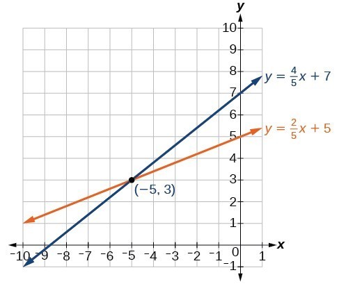
3. [latex]\left(-2,-5\right)[/latex]
4. [latex]\left(-6,-2\right)[/latex]
5. [latex]\left(10,-4\right)[/latex]
6. No solution. It is an inconsistent system.
7. The system is dependent so there are infinite solutions of the form [latex]\left(x,2x+5\right)[/latex].
8. 700 children, 950 adults
1. No, you can either have zero, one, or infinitely many. Examine graphs.
3. This means there is no realistic break-even point. By the time the company produces one unit they are already making profit.
5. You can solve by substitution (isolating [latex]x[/latex] or [latex]y[/latex] ), graphically, or by addition.
7. Yes
9. Yes
11. [latex]\left(-1,2\right)[/latex]
13. [latex]\left(-3,1\right)[/latex]
15. [latex]\left(-\frac{3}{5},0\right)[/latex]
17. No solutions exist.
19. [latex]\left(\frac{72}{5},\frac{132}{5}\right)[/latex]
21. [latex]\left(6,-6\right)[/latex]
23. [latex]\left(-\frac{1}{2},\frac{1}{10}\right)[/latex]
25. No solutions exist.
27. [latex]\left(-\frac{1}{5},\frac{2}{3}\right)[/latex]
29. [latex]\left(x,\frac{x+3}{2}\right)[/latex]
31. [latex]\left(-4,4\right)[/latex]
33. [latex]\left(\frac{1}{2},\frac{1}{8}\right)[/latex]
35. [latex]\left(\frac{1}{6},0\right)[/latex]
37. [latex]\left(x,2\left(7x - 6\right)\right)[/latex]
39. [latex]\left(-\frac{5}{6},\frac{4}{3}\right)[/latex]
41. Consistent with one solution
43. Consistent with one solution
45. Dependent with infinitely many solutions
47. [latex]\left(-3.08,4.91\right)[/latex]
49. [latex]\left(-1.52,2.29\right)[/latex]
51. [latex]\left(\frac{A+B}{2},\frac{A-B}{2}\right)[/latex]
53. [latex]\left(\frac{-1}{A-B},\frac{A}{A-B}\right)[/latex]
55. [latex]\left(\frac{CE-BF}{BD-AE},\frac{AF-CD}{BD-AE}\right)[/latex]
57. They never turn a profit.
59. [latex]\left(1,250,100,000\right)[/latex]
61. The numbers are 7.5 and 20.5.
63. 24,000
65. 790 sophomores, 805 freshman
67. 56 men, 74 women
69. 10 gallons of 10% solution, 15 gallons of 60% solution
71. Swan Peak: $750,000, Riverside: $350,000
73. $12,500 in the first account, $10,500 in the second account.
75. High-tops: 45, Low-tops: 15
77. Infinitely many solutions. We need more information.
By the end of this section, you will be able to:
Figure 1. (credit: “Elembis,” Wikimedia Commons)
John received an inheritance of $12,000 that he divided into three parts and invested in three ways: in a money-market fund paying 3% annual interest; in municipal bonds paying 4% annual interest; and in mutual funds paying 7% annual interest. John invested $4,000 more in municipal funds than in municipal bonds. He earned $670 in interest the first year. How much did John invest in each type of fund?
Understanding the correct approach to setting up problems such as this one makes finding a solution a matter of following a pattern. We will solve this and similar problems involving three equations and three variables in this section. Doing so uses similar techniques as those used to solve systems of two equations in two variables. However, finding solutions to systems of three equations requires a bit more organization and a touch of visual gymnastics.
In order to solve systems of equations in three variables, known as three-by-three systems, the primary tool we will be using is called Gaussian elimination, named after the prolific German mathematician Karl Friedrich Gauss. While there is no definitive order in which operations are to be performed, there are specific guidelines as to what type of moves can be made. We may number the equations to keep track of the steps we apply. The goal is to eliminate one variable at a time to achieve upper triangular form, the ideal form for a three-by-three system because it allows for straightforward back-substitution to find a solution [latex]\left(x,y,z\right),\text{}[/latex] which we call an ordered triple. A system in upper triangular form looks like the following:
The third equation can be solved for [latex]z,\text{}[/latex] and then we back-substitute to find [latex]y[/latex] and [latex]x[/latex]. To write the system in upper triangular form, we can perform the following operations:
The solution set to a three-by-three system is an ordered triple [latex]\left\{\left(x,y,z\right)\right\}[/latex]. Graphically, the ordered triple defines the point that is the intersection of three planes in space. You can visualize such an intersection by imagining any corner in a rectangular room. A corner is defined by three planes: two adjoining walls and the floor (or ceiling). Any point where two walls and the floor meet represents the intersection of three planes.
Figure 2 and Figure 3 illustrate possible solution scenarios for three-by-three systems.
Figure 2. (a)Three planes intersect at a single point, representing a three-by-three system with a single solution. (b) Three planes intersect in a line, representing a three-by-three system with infinite solutions.
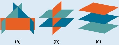
Figure 3
Determine whether the ordered triple [latex]\left(3,-2,1\right)[/latex] is a solution to the system.
We will check each equation by substituting in the values of the ordered triple for [latex]x,y[/latex], and [latex]z[/latex].
[latex]\begin{array}{ccccc}\begin{array}{r}\hfill x+y+z=2\\ \hfill \left(3\right)+\left(-2\right)+\left(1\right)=2\\ \hfill \text{True}\end{array}& & \begin{array}{r}\hfill \text{}6x - 4y+5z=31\\ \hfill 6\left(3\right)-4\left(-2\right)+5\left(1\right)=31\\ \hfill 18+8+5=31\\ \hfill \text{True}\end{array}& & \begin{array}{r}\hfill \text{}5x+2y+2z=13\\ \hfill 5\left(3\right)+2\left(-2\right)+2\left(1\right)=13\\ \hfill \text{}15 - 4+2=13\\ \hfill \text{True}\end{array}\end{array}[/latex]
The ordered triple [latex]\left(3,-2,1\right)[/latex] is indeed a solution to the system.
Find a solution to the following system:
There will always be several choices as to where to begin, but the most obvious first step here is to eliminate [latex]x[/latex] by adding equations (1) and (2).
The second step is multiplying equation (1) by [latex]-2[/latex] and adding the result to equation (3). These two steps will eliminate the variable [latex]x[/latex].
[latex]\begin{array} \hfill−2x+4y−6z=−18 \hfill& \left(1\right)\text{ multiplied by }−2 \\ 2x−5y+5z=17 \hfill& \left(3\right) \\ \text{_____________________________} \\ \hfill−y−z=−1\left(5\right)\hfill& \end{array}[/latex]
In equations (4) and (5), we have created a new two-by-two system. We can solve for [latex]z[/latex] by adding the two equations.
Choosing one equation from each new system, we obtain the upper triangular form:
Next, we back-substitute [latex]z=2[/latex] into equation (4) and solve for [latex]y[/latex].
Finally, we can back-substitute [latex]z=2[/latex] and [latex]y=-1[/latex] into equation (1). This will yield the solution for [latex]x[/latex].
The solution is the ordered triple [latex]\left(1,-1,2\right)[/latex].

Figure 4
In the problem posed at the beginning of the section, John invested his inheritance of $12,000 in three different funds: part in a money-market fund paying 3% interest annually; part in municipal bonds paying 4% annually; and the rest in mutual funds paying 7% annually. John invested $4,000 more in mutual funds than he invested in municipal bonds. The total interest earned in one year was $670. How much did he invest in each type of fund?
To solve this problem, we use all of the information given and set up three equations. First, we assign a variable to each of the three investment amounts:
The first equation indicates that the sum of the three principal amounts is $12,000.
We form the second equation according to the information that John invested $4,000 more in mutual funds than he invested in municipal bonds.
The third equation shows that the total amount of interest earned from each fund equals $670.
Then, we write the three equations as a system.
To make the calculations simpler, we can multiply the third equation by 100. Thus,
Step 1. Interchange equation (2) and equation (3) so that the two equations with three variables will line up.
Step 2. Multiply equation (1) by [latex]-3[/latex] and add to equation (2). Write the result as row 2.
Step 3. Add equation (2) to equation (3) and write the result as equation (3).
Step 4. Solve for [latex]z[/latex] in equation (3). Back-substitute that value in equation (2) and solve for [latex]y[/latex]. Then, back-substitute the values for [latex]z[/latex] and [latex]y[/latex] into equation (1) and solve for [latex]x[/latex].
John invested $2,000 in a money-market fund, $3,000 in municipal bonds, and $7,000 in mutual funds.
Solve the system of equations in three variables.
Just as with systems of equations in two variables, we may come across an inconsistent system of equations in three variables, which means that it does not have a solution that satisfies all three equations. The equations could represent three parallel planes, two parallel planes and one intersecting plane, or three planes that intersect the other two but not at the same location. The process of elimination will result in a false statement, such as [latex]3=7[/latex] or some other contradiction.
Solve the following system.
Looking at the coefficients of [latex]x[/latex], we can see that we can eliminate [latex]x[/latex] by adding equation (1) to equation (2).
Next, we multiply equation (1) by [latex]-5[/latex] and add it to equation (3).
[latex]\begin{array}−5x+15y−5z=−20 \hfill& \left(1\right)\text{ multiplied by }−5 \\ 5x−13y+13z=8 \hfill& \left(3\right) \\ \text{___________________} \\ 2y+8z=−12\hfill&\left(5\right) \end{array}[/latex]
Then, we multiply equation (4) by 2 and add it to equation (5).
The final equation [latex]0=2[/latex] is a contradiction, so we conclude that the system of equations in inconsistent and, therefore, has no solution.
In this system, each plane intersects the other two, but not at the same location. Therefore, the system is inconsistent.
Solve the system of three equations in three variables.
We know from working with systems of equations in two variables that a dependent system of equations has an infinite number of solutions. The same is true for dependent systems of equations in three variables. An infinite number of solutions can result from several situations. The three planes could be the same, so that a solution to one equation will be the solution to the other two equations. All three equations could be different but they intersect on a line, which has infinite solutions. Or two of the equations could be the same and intersect the third on a line.
Find the solution to the given system of three equations in three variables.
First, we can multiply equation (1) by [latex]-2[/latex] and add it to equation (2).
[latex]\begin{array} −4x−2y+6z=0 \hfill& \text{equation }\left(1\right)\text{multiplied by }−2 \\ 4x+2y−6z=0\hfill&\left(2\right) \end{array}[/latex]
We do not need to proceed any further. The result we get is an identity, [latex]0=0[/latex], which tells us that this system has an infinite number of solutions. There are other ways to begin to solve this system, such as multiplying equation (3) by [latex]-2[/latex], and adding it to equation (1). We then perform the same steps as above and find the same result, [latex]0=0[/latex].
When a system is dependent, we can find general expressions for the solutions. Adding equations (1) and (3), we have
[latex]\begin{array}2x+y−3z=0 \\ x−y+z=0 \\ \text{______________} \\ 3x−2z=0 \end{array}[/latex]
We then solve the resulting equation for [latex]z[/latex].
We back-substitute the expression for [latex]z[/latex] into one of the equations and solve for [latex]y[/latex].
So the general solution is [latex]\left(x,\frac{5}{2}x,\frac{3}{2}x\right)[/latex]. In this solution, [latex]x[/latex] can be any real number. The values of [latex]y[/latex] and [latex]z[/latex] are dependent on the value selected for [latex]x[/latex].
As shown in Figure 5, two of the planes are the same and they intersect the third plane on a line. The solution set is infinite, as all points along the intersection line will satisfy all three equations.
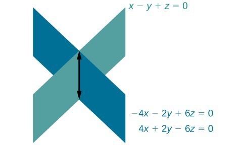
Figure 5
No, you can write the generic solution in terms of any of the variables, but it is common to write it in terms of x and if needed [latex]x[/latex] and [latex]y[/latex].
Solve the following system.
1. Can a linear system of three equations have exactly two solutions? Explain why or why not
2. If a given ordered triple solves the system of equations, is that solution unique? If so, explain why. If not, give an example where it is not unique.
3. If a given ordered triple does not solve the system of equations, is there no solution? If so, explain why. If not, give an example.
4. Using the method of addition, is there only one way to solve the system?
5. Can you explain whether there can be only one method to solve a linear system of equations? If yes, give an example of such a system of equations. If not, explain why not.
For the following exercises, determine whether the ordered triple given is the solution to the system of equations.
6. [latex]\begin{array}{l}2x - 6y+6z=-12\hfill \\ \text{ }x+4y+5z=-1\hfill \\ \mathrm{-x}+2y+3z=-1\hfill \end{array}[/latex] and [latex]\left(0,1,-1\right)[/latex]
7. [latex]\begin{array}{l}\text{ }6x-y+3z=6\hfill \\ 3x+5y+2z=0\hfill \\ \text{ }x+y=0\hfill \end{array}[/latex] and [latex]\left(3,-3,-5\right)[/latex]
8. [latex]\begin{array}{l}6x - 7y+z=2\hfill \\ \mathrm{-x}-y+3z=4\hfill \\ \text{ }2x+y-z=1\hfill \end{array}[/latex] and [latex]\left(4,2,-6\right)[/latex]
9. [latex]\begin{array}{l}\text{ }x-y=0\hfill \\ \text{ }x-z=5\hfill \\ x-y+z=-1\hfill \end{array}[/latex] and [latex]\left(4,4,-1\right)[/latex]
10. [latex]\begin{array}{l} \mathrm{-x}-y+2z=3\hfill \\ \text{ }5x+8y - 3z=4\hfill \\ \mathrm{-x}+3y - 5z=-5\hfill \end{array}[/latex] and [latex]\left(4,1,-7\right)[/latex]
For the following exercises, solve each system by substitution.
11. [latex]\begin{array}{l}3x - 4y+2z=-15\hfill \\ \text{ }2x+4y+z=16\hfill \\ \text{ }2x+3y+5z=20\hfill \end{array}[/latex]
12. [latex]\begin{array}{l}5x - 2y+3z=20\hfill \\ 2x - 4y - 3z=-9\hfill \\ \text{ }x+6y - 8z=21\hfill \end{array}[/latex]
13. [latex]\begin{array}{l}\text{ }5x+2y+4z=9\hfill \\ -3x+2y+z=10\hfill \\ \text{ }4x - 3y+5z=-3\hfill \end{array}[/latex]
14. [latex]\begin{array}{l}4x - 3y+5z=31\hfill \\ -x+2y+4z=20\hfill \\ \text{ }x+5y - 2z=-29\hfill \end{array}[/latex]
15. [latex]\begin{array}{l}\text{ }5x - 2y+3z=4\hfill \\ -4x+6y - 7z=-1\hfill \\ \text{ }3x+2y-z=4\hfill \end{array}[/latex]
16. [latex]\begin{array}{l} 4x+6y+9z=0\hfill \\ -5x+2y - 6z=3\hfill \\ 7x - 4y+3z=-3\hfill \end{array}[/latex]
For the following exercises, solve each system by Gaussian elimination.
17. [latex]\begin{array}{l}\text{ }2x-y+3z=17\hfill \\ -5x+4y - 2z=-46\hfill \\ \text{ }2y+5z=-7\hfill \end{array}[/latex]
18. [latex]\begin{array}{l}5x - 6y+3z=50\hfill \\ \text{ }-x+4y=10\hfill \\ \text{ }2x-z=10\hfill \end{array}[/latex]
19. [latex]\begin{array}{l}\text{ }2x+3y - 6z=1\hfill \\ -4x - 6y+12z=-2\hfill \\ \text{ }x+2y+5z=10\hfill \end{array}[/latex]
20. [latex]\begin{array}{l}\text{ }4x+6y - 2z=8\hfill \\ \text{ }6x+9y - 3z=12\hfill \\ -2x - 3y+z=-4\hfill \end{array}[/latex]
21. [latex]\begin{array}{l}2x+3y - 4z=5\hfill \\ -3x+2y+z=11\hfill \\ -x+5y+3z=4\hfill \end{array}[/latex]
22. [latex]\begin{array}{l}10x+2y - 14z=8\hfill \\ \text{ }\mathrm{-x}-2y - 4z=-1\hfill \\ -12x - 6y+6z=-12\hfill \end{array}[/latex]
23. [latex]\begin{array}{l}\text{ }x+y+z=14\hfill \\ \text{ }2y+3z=-14\hfill \\ -16y - 24z=-112\hfill \end{array}[/latex]
24. [latex]\begin{array}{l}\text{ }5x - 3y+4z=-1\hfill \\ -4x+2y - 3z=0\hfill \\ \text{ }\mathrm{-x}+5y+7z=-11\hfill \end{array}[/latex]
25. [latex]\begin{array}{l}\text{ }x+y+z=0\hfill \\ \text{ }2x-y+3z=0\hfill \\ \text{ }x-z=0\hfill \end{array}[/latex]
26. [latex]\begin{array}{l}3x+2y - 5z=6\\ 5x - 4y+3z=-12\\ 4x+5y - 2z=15\end{array}[/latex]
27. [latex]\begin{array}{l}\text{ }x+y+z=0\hfill \\ 2x-y+3z=0\hfill \\ \text{ }x-z=1\hfill \end{array}[/latex]
28. [latex]\begin{array}{l}\begin{array}{l}\\ 3x-\frac{1}{2}y-z=-\frac{1}{2}\end{array}\hfill \\ \text{ }4x+z=3\hfill \\ \text{ }-x+\frac{3}{2}y=\frac{5}{2}\hfill \end{array}[/latex]
29. [latex]\begin{array}{l}\text{ }6x - 5y+6z=38\hfill \\ \frac{1}{5}x-\frac{1}{2}y+\frac{3}{5}z=1\hfill \\ \text{ }-4x-\frac{3}{2}y-z=-74\hfill \end{array}[/latex]
30. [latex]\begin{array}{l}\frac{1}{2}x-\frac{1}{5}y+\frac{2}{5}z=-\frac{13}{10}\hfill \\ \frac{1}{4}x-\frac{2}{5}y-\frac{1}{5}z=-\frac{7}{20}\hfill \\ -\frac{1}{2}x-\frac{3}{4}y-\frac{1}{2}z=-\frac{5}{4}\hfill \end{array}[/latex]
31. [latex]\begin{array}{l}\begin{array}{l}\\ -\frac{1}{3}x-\frac{1}{2}y-\frac{1}{4}z=\frac{3}{4}\end{array}\hfill \\ -\frac{1}{2}x-\frac{1}{4}y-\frac{1}{2}z=2\hfill \\ -\frac{1}{4}x-\frac{3}{4}y-\frac{1}{2}z=-\frac{1}{2}\hfill \end{array}[/latex]
32. [latex]\begin{array}{l}\frac{1}{2}x-\frac{1}{4}y+\frac{3}{4}z=0\\ \frac{1}{4}x-\frac{1}{10}y+\frac{2}{5}z=-2\\ \frac{1}{8}x+\frac{1}{5}y-\frac{1}{8}z=2\end{array}[/latex]
33. [latex]\begin{array}{l}\text{ }\frac{4}{5}x-\frac{7}{8}y+\frac{1}{2}z=1\hfill \\ -\frac{4}{5}x-\frac{3}{4}y+\frac{1}{3}z=-8\hfill \\ -\frac{2}{5}x-\frac{7}{8}y+\frac{1}{2}z=-5\hfill \end{array}[/latex]
34. [latex]\begin{array}{l}\begin{array}{l}\\ -\frac{1}{3}x-\frac{1}{8}y+\frac{1}{6}z=-\frac{4}{3}\end{array}\hfill \\ -\frac{2}{3}x-\frac{7}{8}y+\frac{1}{3}z=-\frac{23}{3}\hfill \\ -\frac{1}{3}x-\frac{5}{8}y+\frac{5}{6}z=0\hfill \end{array}[/latex]
35. [latex]\begin{array}{l}\begin{array}{l}\\ -\frac{1}{4}x-\frac{5}{4}y+\frac{5}{2}z=-5\end{array}\hfill \\ -\frac{1}{2}x-\frac{5}{3}y+\frac{5}{4}z=\frac{55}{12}\hfill \\ -\frac{1}{3}x-\frac{1}{3}y+\frac{1}{3}z=\frac{5}{3}\hfill \end{array}[/latex]
36. [latex]\begin{array}{l}\frac{1}{40}x+\frac{1}{60}y+\frac{1}{80}z=\frac{1}{100}\hfill \\ -\frac{1}{2}x-\frac{1}{3}y-\frac{1}{4}z=-\frac{1}{5}\hfill \\ \frac{3}{8}x+\frac{3}{12}y+\frac{3}{16}z=\frac{3}{20}\hfill \end{array}[/latex]
37. [latex]\begin{array}{l}0.1x - 0.2y+0.3z=2\\ 0.5x - 0.1y+0.4z=8\\ 0.7x - 0.2y+0.3z=8\end{array}[/latex]
38. [latex]\begin{array}{l}0.2x+0.1y - 0.3z=0.2\\ 0.8x+0.4y - 1.2z=0.1\\ 1.6x+0.8y - 2.4z=0.2\end{array}[/latex]
39. [latex]\begin{array}{l}1.1x+0.7y - 3.1z=-1.79\\ 2.1x+0.5y - 1.6z=-0.13\\ 0.5x+0.4y - 0.5z=-0.07\end{array}[/latex]
40. [latex]\begin{array}{l}0.5x - 0.5y+0.5z=10\\ 0.2x - 0.2y+0.2z=4\\ 0.1x - 0.1y+0.1z=2\end{array}[/latex]
41. [latex]\begin{array}{l}0.1x+0.2y+0.3z=0.37\\ 0.1x - 0.2y - 0.3z=-0.27\\ 0.5x - 0.1y - 0.3z=-0.03\end{array}[/latex]
42. [latex]\begin{array}{l}0.5x - 0.5y - 0.3z=0.13\\ 0.4x - 0.1y - 0.3z=0.11\\ 0.2x - 0.8y - 0.9z=-0.32\end{array}[/latex]
43. [latex]\begin{array}{l}0.5x+0.2y - 0.3z=1\\ 0.4x - 0.6y+0.7z=0.8\\ 0.3x - 0.1y - 0.9z=0.6\end{array}[/latex]
44. [latex]\begin{array}{l}0.3x+0.3y+0.5z=0.6\\ 0.4x+0.4y+0.4z=1.8\\ 0.4x+0.2y+0.1z=1.6\end{array}[/latex]
45. [latex]\begin{array}{l}0.8x+0.8y+0.8z=2.4\\ 0.3x - 0.5y+0.2z=0\\ 0.1x+0.2y+0.3z=0.6\end{array}[/latex]
For the following exercises, solve the system for [latex]x,y[/latex], and [latex]z[/latex].
46. [latex]\begin{array}{l}\text{ }x+y+z=3\hfill \\ \frac{x - 1}{2}+\frac{y - 3}{2}+\frac{z+1}{2}=0\hfill \\ \frac{x - 2}{3}+\frac{y+4}{3}+\frac{z - 3}{3}=\frac{2}{3}\hfill \end{array}[/latex]
47. [latex]\begin{array}{l}5x - 3y-\frac{z+1}{2}=\frac{1}{2}\hfill \\ 6x+\frac{y - 9}{2}+2z=-3\hfill \\ \text{ }\frac{x+8}{2}-4y+z=4\hfill \end{array}[/latex]
48. [latex]\begin{array}{l}\frac{x+4}{7}-\frac{y - 1}{6}+\frac{z+2}{3}=1\\ \frac{x - 2}{4}+\frac{y+1}{8}-\frac{z+8}{12}=0\\ \frac{x+6}{3}-\frac{y+2}{3}+\frac{z+4}{2}=3\end{array}[/latex]
49. [latex]\begin{array}{l}\frac{x - 3}{6}+\frac{y+2}{2}-\frac{z - 3}{3}=2\\ \frac{x+2}{4}+\frac{y - 5}{2}+\frac{z+4}{2}=1\\ \frac{x+6}{2}-\frac{y - 3}{2}+z+1=9\end{array}[/latex]
50. [latex]\begin{array}{l}\text{ }\frac{x - 1}{3}+\frac{y+3}{4}+\frac{z+2}{6}=1\hfill \\ \text{ }4x+3y - 2z=11\hfill \\ 0.02x+0.015y - 0.01z=0.065\hfill \end{array}[/latex]
51. Three even numbers sum up to 108. The smaller is half the larger and the middle number is [latex]\frac{3}{4}[/latex]
the larger. What are the three numbers?
52. Three numbers sum up to 147. The smallest number is half the middle number, which is half the largest number. What are the three numbers?
53. At a family reunion, there were only blood relatives, consisting of children, parents, and grandparents, in attendance. There were 400 people total. There were twice as many parents as grandparents, and 50 more children than parents. How many children, parents, and grandparents were in attendance?
54. An animal shelter has a total of 350 animals comprised of cats, dogs, and rabbits. If the number of rabbits is 5 less than one-half the number of cats, and there are 20 more cats than dogs, how many of each animal are at the shelter?
55. Your roommate, Sarah, offered to buy groceries for you and your other roommate. The total bill was $82. She forgot to save the individual receipts but remembered that your groceries were $0.05 cheaper than half of her groceries, and that your other roommate’s groceries were $2.10 more than your groceries. How much was each of your share of the groceries?
56. Your roommate, John, offered to buy household supplies for you and your other roommate. You live near the border of three states, each of which has a different sales tax. The total amount of money spent was $100.75. Your supplies were bought with 5% tax, John’s with 8% tax, and your third roommate’s with 9% sales tax. The total amount of money spent without taxes is $93.50. If your supplies before tax were $1 more than half of what your third roommate’s supplies were before tax, how much did each of you spend? Give your answer both with and without taxes.
57. Three coworkers work for the same employer. Their jobs are warehouse manager, office manager, and truck driver. The sum of the annual salaries of the warehouse manager and office manager is $82,000. The office manager makes $4,000 more than the truck driver annually. The annual salaries of the warehouse manager and the truck driver total $78,000. What is the annual salary of each of the co-workers?
58. At a carnival, $2,914.25 in receipts were taken at the end of the day. The cost of a child’s ticket was $20.50, an adult ticket was $29.75, and a senior citizen ticket was $15.25. There were twice as many senior citizens as adults in attendance, and 20 more children than senior citizens. How many children, adult, and senior citizen tickets were sold?
59. A local band sells out for their concert. They sell all 1,175 tickets for a total purse of $28,112.50. The tickets were priced at $20 for student tickets, $22.50 for children, and $29 for adult tickets. If the band sold twice as many adult as children tickets, how many of each type was sold?
60. In a bag, a child has 325 coins worth $19.50. There were three types of coins: pennies, nickels, and dimes. If the bag contained the same number of nickels as dimes, how many of each type of coin was in the bag?
61. Last year, at Haven’s Pond Car Dealership, for a particular model of BMW, Jeep, and Toyota, one could purchase all three cars for a total of $140,000. This year, due to inflation, the same cars would cost $151,830. The cost of the BMW increased by 8%, the Jeep by 5%, and the Toyota by 12%. If the price of last year’s Jeep was $7,000 less than the price of last year’s BMW, what was the price of each of the three cars last year?
62. A recent college graduate took advantage of his business education and invested in three investments immediately after graduating. He invested $80,500 into three accounts, one that paid 4% simple interest, one that paid [latex]3\frac{1}{8}\text{%}[/latex] simple interest, and one that paid [latex]2\frac{1}{2}\text{%}[/latex] simple interest. He earned $2,670 interest at the end of one year. If the amount of the money invested in the second account was four times the amount invested in the third account, how much was invested in each account?
63. You inherit one million dollars. You invest it all in three accounts for one year. The first account pays 3% compounded annually, the second account pays 4% compounded annually, and the third account pays 2% compounded annually. After one year, you earn $34,000 in interest. If you invest four times the money into the account that pays 3% compared to 2%, how much did you invest in each account?
64. You inherit one hundred thousand dollars. You invest it all in three accounts for one year. The first account pays 4% compounded annually, the second account pays 3% compounded annually, and the third account pays 2% compounded annually. After one year, you earn $3,650 in interest. If you invest five times the money in the account that pays 4% compared to 3%, how much did you invest in each account?
65. The top three countries in oil consumption in a certain year are as follows: the United States, Japan, and China. In millions of barrels per day, the three top countries consumed 39.8% of the world’s consumed oil. The United States consumed 0.7% more than four times China’s consumption. The United States consumed 5% more than triple Japan’s consumption. What percent of the world oil consumption did the United States, Japan, and China consume? (“Oil reserves, production and consumption in 2001,” accessed April 6, 2014, http://scaruffi.com/politics/oil.html)
66. The top three countries in oil production in the same year are Saudi Arabia, the United States, and Russia. In millions of barrels per day, the top three countries produced 31.4% of the world’s produced oil. Saudi Arabia and the United States combined for 22.1% of the world’s production, and Saudi Arabia produced 2% more oil than Russia. What percent of the world oil production did Saudi Arabia, the United States, and Russia produce? (“Oil reserves, production and consumption in 2001,” accessed April 6, 2014, http://scaruffi.com/politics/oil.html)
67. The top three sources of oil imports for the United States in the same year were Saudi Arabia, Mexico, and Canada. The three top countries accounted for 47% of oil imports. The United States imported 1.8% more from Saudi Arabia than they did from Mexico, and 1.7% more from Saudi Arabia than they did from Canada. What percent of the United States oil imports were from these three countries? (“Oil reserves, production and consumption in 2001,” accessed April 6, 2014, http://scaruffi.com/politics/oil.html)
68. The top three oil producers in the United States in a certain year are the Gulf of Mexico, Texas, and Alaska. The three regions were responsible for 64% of the United States oil production. The Gulf of Mexico and Texas combined for 47% of oil production. Texas produced 3% more than Alaska. What percent of United States oil production came from these regions? (“USA: The coming global oil crisis,” accessed April 6, 2014, http://www.oilcrisis.com/us/)
69. At one time, in the United States, 398 species of animals were on the endangered species list. The top groups were mammals, birds, and fish, which comprised 55% of the endangered species. Birds accounted for 0.7% more than fish, and fish accounted for 1.5% more than mammals. What percent of the endangered species came from mammals, birds, and fish?
70. Meat consumption in the United States can be broken into three categories: red meat, poultry, and fish. If fish makes up 4% less than one-quarter of poultry consumption, and red meat consumption is 18.2% higher than poultry consumption, what are the percentages of meat consumption? (“The United States Meat Industry at a Glance,” accessed April 6, 2014, http://www.meatami.com/ht/d/sp/i/47465/pid/47465)
1. [latex]\left(1,-1,1\right)[/latex]
2. No solution.
3. Infinite number of solutions of the form [latex]\left(x,4x - 11,-5x+18\right)[/latex].
1. No, there can be only one, zero, or infinitely many solutions.
3. Not necessarily. There could be zero, one, or infinitely many solutions. For example, [latex]\left(0,0,0\right)[/latex] is not a solution to the system below, but that does not mean that it has no solution.
[latex]\begin{array}{l}\text{ }2x+3y - 6z=1\hfill \\ -4x - 6y+12z=-2\hfill \\ \text{ }x+2y+5z=10\hfill \end{array}[/latex]
5. Every system of equations can be solved graphically, by substitution, and by addition. However, systems of three equations become very complex to solve graphically so other methods are usually preferable.
7. No
9. Yes
11. [latex]\left(-1,4,2\right)[/latex]
13. [latex]\left(-\frac{85}{107},\frac{312}{107},\frac{191}{107}\right)[/latex]
15. [latex]\left(1,\frac{1}{2},0\right)[/latex]
17. [latex]\left(4,-6,1\right)[/latex]
19. [latex]\left(x,\frac{1}{27}\left(65 - 16x\right),\frac{x+28}{27}\right)[/latex]
21. [latex]\left(-\frac{45}{13},\frac{17}{13},-2\right)[/latex]
23. No solutions exist
25. [latex]\left(0,0,0\right)[/latex]
27. [latex]\left(\frac{4}{7},-\frac{1}{7},-\frac{3}{7}\right)[/latex]
29. [latex]\left(7,20,16\right)[/latex]
31. [latex]\left(-6,2,1\right)[/latex]
33. [latex]\left(5,12,15\right)[/latex]
35. [latex]\left(-5,-5,-5\right)[/latex]
37. [latex]\left(10,10,10\right)[/latex]
39. [latex]\left(\frac{1}{2},\frac{1}{5},\frac{4}{5}\right)[/latex]
41. [latex]\left(\frac{1}{2},\frac{2}{5},\frac{4}{5}\right)[/latex]
43. [latex]\left(2,0,0\right)[/latex]
45. [latex]\left(1,1,1\right)[/latex]
47. [latex]\left(\frac{128}{557},\frac{23}{557},\frac{28}{557}\right)[/latex]
49. [latex]\left(6,-1,0\right)[/latex]
51. 24, 36, 48
53. 70 grandparents, 140 parents, 190 children
55. Your share was $19.95, Sarah’s share was $40, and your other roommate’s share was $22.05.
57. There are infinitely many solutions; we need more information
59. 500 students, 225 children, and 450 adults
61. The BMW was $49,636, the Jeep was $42,636, and the Toyota was $47,727.
63. $400,000 in the account that pays 3% interest, $500,000 in the account that pays 4% interest, and $100,000 in the account that pays 2% interest.
65. The United States consumed 26.3%, Japan 7.1%, and China 6.4% of the world’s oil.
67. Saudi Arabia imported 16.8%, Canada imported 15.1%, and Mexico 15.0%
69. Birds were 19.3%, fish were 18.6%, and mammals were 17.1% of endangered species
By the end of this section, you will be able to:
Halley’s Comet orbits the sun about once every 75 years. Its path can be considered to be a very elongated ellipse. Other comets follow similar paths in space. These orbital paths can be studied using systems of equations. These systems, however, are different from the ones we considered in the previous section because the equations are not linear.
Figure 1. Halley’s Comet (credit: “NASA Blueshift”/Flickr)
In this section, we will consider the intersection of a parabola and a line, a circle and a line, and a circle and an ellipse. The methods for solving systems of nonlinear equations are similar to those for linear equations.
A system of nonlinear equations is a system of two or more equations in two or more variables containing at least one equation that is not linear. Recall that a linear equation can take the form [latex]Ax+By+C=0[/latex]. Any equation that cannot be written in this form in nonlinear. The substitution method we used for linear systems is the same method we will use for nonlinear systems. We solve one equation for one variable and then substitute the result into the second equation to solve for another variable, and so on. There is, however, a variation in the possible outcomes.
There are three possible types of solutions for a system of nonlinear equations involving a parabola and a line.
Figure 2 illustrates possible solution sets for a system of equations involving a parabola and a line.
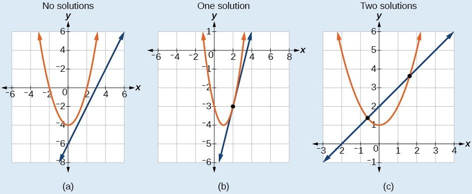
Figure 2
Solve the system of equations.
Solve the first equation for [latex]x[/latex] and then substitute the resulting expression into the second equation.
Expand the equation and set it equal to zero.
Solving for [latex]y[/latex] gives [latex]y=2[/latex] and [latex]y=1[/latex]. Next, substitute each value for [latex]y[/latex] into the first equation to solve for [latex]x[/latex]. Always substitute the value into the linear equation to check for extraneous solutions.
The solutions are [latex]\left(1,2\right)[/latex] and [latex]\left(0,1\right),\text{}[/latex] which can be verified by substituting these [latex]\left(x,y\right)[/latex] values into both of the original equations.
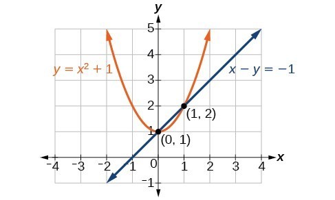
Figure 3
Yes, but because [latex]x[/latex] is squared in the second equation this could give us extraneous solutions for [latex]x[/latex].
For [latex]y=1[/latex]
This gives us the same value as in the solution.
For [latex]y=2[/latex]
Notice that [latex]-1[/latex] is an extraneous solution.
Solve the given system of equations by substitution.
Just as with a parabola and a line, there are three possible outcomes when solving a system of equations representing a circle and a line.
Figure 4 illustrates possible solution sets for a system of equations involving a circle and a line.
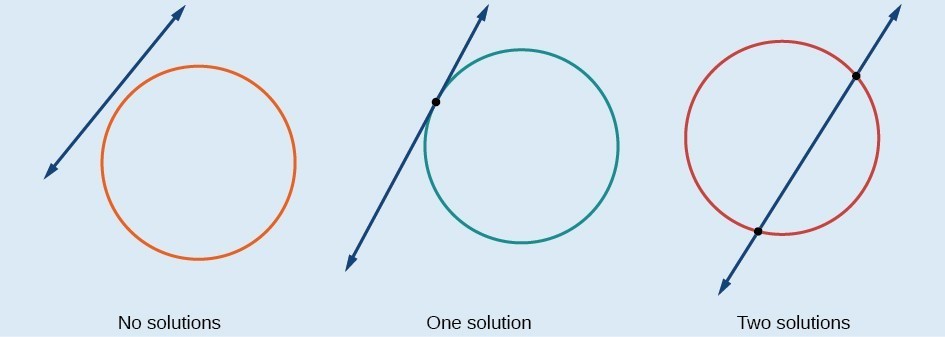
Figure 4
Find the intersection of the given circle and the given line by substitution.
One of the equations has already been solved for [latex]y[/latex]. We will substitute [latex]y=3x - 5[/latex] into the equation for the circle.
Now, we factor and solve for [latex]x[/latex].
Substitute the two x-values into the original linear equation to solve for [latex]y[/latex].
The line intersects the circle at [latex]\left(2,1\right)[/latex] and [latex]\left(1,-2\right)[/latex], which can be verified by substituting these [latex]\left(x,y\right)[/latex] values into both of the original equations.
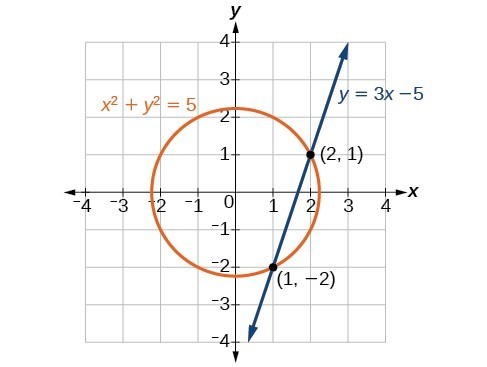
Figure 5
Solve the system of nonlinear equations.
We have seen that substitution is often the preferred method when a system of equations includes a linear equation and a nonlinear equation. However, when both equations in the system have like variables of the second degree, solving them using elimination by addition is often easier than substitution. Generally, elimination is a far simpler method when the system involves only two equations in two variables (a two-by-two system), rather than a three-by-three system, as there are fewer steps. As an example, we will investigate the possible types of solutions when solving a system of equations representing a circle and an ellipse.
Figure 6 illustrates possible solution sets for a system of equations involving a circle and an ellipse.
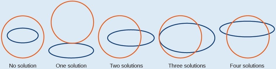
Figure 6
Solve the system of nonlinear equations.
Let’s begin by multiplying equation (1) by [latex]-3,\text{}[/latex] and adding it to equation (2).
After we add the two equations together, we solve for [latex]y[/latex].
Substitute [latex]y=\pm 1[/latex] into one of the equations and solve for [latex]x[/latex].
There are four solutions: [latex]\left(5,1\right),\left(-5,1\right),\left(5,-1\right),\text{and}\left(-5,-1\right)[/latex].
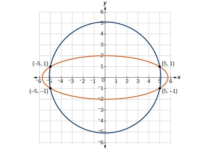
Figure 7
Find the solution set for the given system of nonlinear equations.
All of the equations in the systems that we have encountered so far have involved equalities, but we may also encounter systems that involve inequalities. We have already learned to graph linear inequalities by graphing the corresponding equation, and then shading the region represented by the inequality symbol. Now, we will follow similar steps to graph a nonlinear inequality so that we can learn to solve systems of nonlinear inequalities. A nonlinear inequality is an inequality containing a nonlinear expression. Graphing a nonlinear inequality is much like graphing a linear inequality.
Recall that when the inequality is greater than, [latex]y>a[/latex], or less than, [latex]y<a,\text{}[/latex] the graph is drawn with a dashed line. When the inequality is greater than or equal to, [latex]y\ge a,\text{}[/latex] or less than or equal to, [latex]y\le a,\text{}[/latex] the graph is drawn with a solid line. The graphs will create regions in the plane, and we will test each region for a solution. If one point in the region works, the whole region works. That is the region we shade.
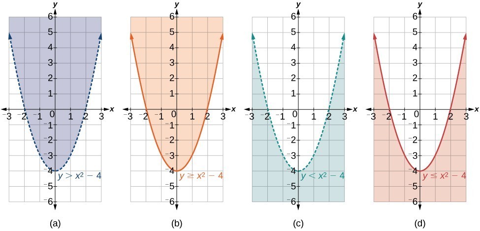
Figure 8. (a) an example of [latex]y>a[/latex]; (b) an example of [latex]y\ge a[/latex]; (c) an example of [latex]y<a[/latex]; (d) an example of [latex]y\le a[/latex]
Graph the inequality [latex]y>{x}^{2}+1[/latex].
First, graph the corresponding equation [latex]y={x}^{2}+1[/latex]. Since [latex]y>{x}^{2}+1[/latex] has a greater than symbol, we draw the graph with a dashed line. Then we choose points to test both inside and outside the parabola. Let’s test the points [latex]\left(0,2\right)[/latex] and [latex]\left(2,0\right)[/latex]. One point is clearly inside the parabola and the other point is clearly outside.
The graph is shown in Figure 9. We can see that the solution set consists of all points inside the parabola, but not on the graph itself.
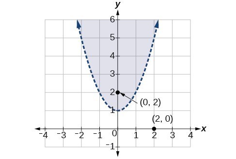
Figure 9
Now that we have learned to graph nonlinear inequalities, we can learn how to graph systems of nonlinear inequalities. A system of nonlinear inequalities is a system of two or more inequalities in two or more variables containing at least one inequality that is not linear. Graphing a system of nonlinear inequalities is similar to graphing a system of linear inequalities. The difference is that our graph may result in more shaded regions that represent a solution than we find in a system of linear inequalities. The solution to a nonlinear system of inequalities is the region of the graph where the shaded regions of the graph of each inequality overlap, or where the regions intersect, called the feasible region.
Graph the given system of inequalities.
These two equations are clearly parabolas. We can find the points of intersection by the elimination process: Add both equations and the variable [latex]y[/latex] will be eliminated. Then we solve for [latex]x[/latex].
[latex]\begin{array}\hfill x^{2}−y=0 \\ 2x^{2}+y=12 \\ \text{___________} \\ 3x^{2}=12 \\ x^{2}=4 \\ x=\pm 2\end{array}[/latex]
Substitute the x-values into one of the equations and solve for [latex]y[/latex].
The two points of intersection are [latex]\left(2,4\right)[/latex] and [latex]\left(-2,4\right)[/latex]. Notice that the equations can be rewritten as follows.
Graph each inequality. The feasible region is the region between the two equations bounded by [latex]2{x}^{2}+y\le 12[/latex] on the top and [latex]{x}^{2}-y\le 0[/latex] on the bottom.
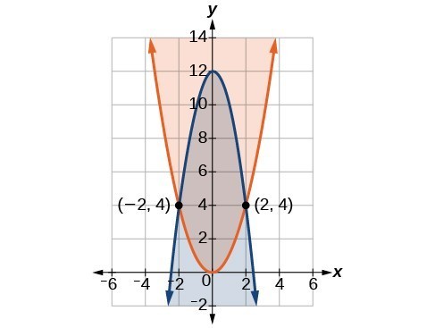
Figure 10
Graph the given system of inequalities.
1. Explain whether a system of two nonlinear equations can have exactly two solutions. What about exactly three? If not, explain why not. If so, give an example of such a system, in graph form, and explain why your choice gives two or three answers.
2. When graphing an inequality, explain why we only need to test one point to determine whether an entire region is the solution?
3. When you graph a system of inequalities, will there always be a feasible region? If so, explain why. If not, give an example of a graph of inequalities that does not have a feasible region. Why does it not have a feasible region?
4. If you graph a revenue and cost function, explain how to determine in what regions there is profit.
5. If you perform your break-even analysis and there is more than one solution, explain how you would determine which x-values are profit and which are not.
For the following exercises, solve the system of nonlinear equations using substitution.
6. [latex]\begin{array}{l}\text{ }x+y=4\hfill \\ {x}^{2}+{y}^{2}=9\hfill \end{array}[/latex]
7. [latex]\begin{array}{l}\text{ }y=x - 3\hfill \\ {x}^{2}+{y}^{2}=9\hfill \end{array}[/latex]
8. [latex]\begin{array}{l}\text{ }y=x\hfill \\ {x}^{2}+{y}^{2}=9\hfill \end{array}[/latex]
9. [latex]\begin{array}{l}\text{ }y=-x\hfill \\ {x}^{2}+{y}^{2}=9\hfill \end{array}[/latex]
10. [latex]\begin{array}{l}\text{ }x=2\hfill \\ {x}^{2}-{y}^{2}=9\hfill \end{array}[/latex]
For the following exercises, solve the system of nonlinear equations using elimination.
11. [latex]\begin{array}{l}\hfill \\ 4{x}^{2}-9{y}^{2}=36\hfill \\ 4{x}^{2}+9{y}^{2}=36\hfill \end{array}[/latex]
12. [latex]\begin{array}{l}{x}^{2}+{y}^{2}=25\\ {x}^{2}-{y}^{2}=1\end{array}[/latex]
13. [latex]\begin{array}{l}\hfill \\ 2{x}^{2}+4{y}^{2}=4\hfill \\ 2{x}^{2}-4{y}^{2}=25x - 10\hfill \end{array}[/latex]
14. [latex]\begin{array}{l}{y}^{2}-{x}^{2}=9\\ 3{x}^{2}+2{y}^{2}=8\end{array}[/latex]
15. [latex]\begin{array}{l}{x}^{2}+{y}^{2}+\frac{1}{16}=2500\\ y=2{x}^{2}\end{array}[/latex]
For the following exercises, use any method to solve the system of nonlinear equations.
16. [latex]\begin{array}{l}\begin{array}{l}\\ -2{x}^{2}+y=-5\end{array}\hfill \\ \text{ }6x-y=9\hfill \end{array}[/latex]
17. [latex]\begin{array}{l}\begin{array}{l}\\ -{x}^{2}+y=2\end{array}\hfill \\ \text{ }-x+y=2\hfill \end{array}[/latex]
18. [latex]\begin{array}{l}{x}^{2}+{y}^{2}=1\hfill \\ \text{ }y=20{x}^{2}-1\hfill \end{array}[/latex]
19. [latex]\begin{array}{l}{x}^{2}+{y}^{2}=1\hfill \\ \text{ }y=-{x}^{2}\hfill \end{array}[/latex]
20. [latex]\begin{array}{l}2{x}^{3}-{x}^{2}=y\hfill \\ \text{ }y=\frac{1}{2}-x\hfill \end{array}[/latex]
21. [latex]\begin{array}{l}9{x}^{2}+25{y}^{2}=225\hfill \\ {\left(x - 6\right)}^{2}+{y}^{2}=1\hfill \end{array}[/latex]
22. [latex]\begin{array}{l}{x}^{4}-{x}^{2}=y\hfill \\ \text{ }{x}^{2}+y=0\hfill \end{array}[/latex]
23. [latex]\begin{array}{l}2{x}^{3}-{x}^{2}=y\hfill \\ \text{ }{x}^{2}+y=0\hfill \end{array}[/latex]
For the following exercises, use any method to solve the nonlinear system.
24. [latex]\begin{array}{l}{x}^{2}+{y}^{2}=9\hfill \\ \text{ }y=3-{x}^{2}\hfill \end{array}[/latex]
25. [latex]\begin{array}{l}{x}^{2}-{y}^{2}=9\hfill \\ \text{ }x=3\hfill \end{array}[/latex]
26. [latex]\begin{array}{l}{x}^{2}-{y}^{2}=9\hfill \\ \text{ }y=3\hfill \end{array}[/latex]
27. [latex]\begin{array}{l}{x}^{2}-{y}^{2}=9\hfill \\ \text{ }x-y=0\hfill \end{array}[/latex]
28. [latex]\begin{array}{l}\hfill \\ -{x}^{2}+y=2\hfill \\ -4x+y=-1\hfill \end{array}[/latex]
29. [latex]\begin{array}{l}-{x}^{2}+y=2\hfill \\ \text{ }2y=-x\hfill \end{array}[/latex]
30. [latex]\begin{array}{l}{x}^{2}+{y}^{2}=25\\ {x}^{2}-{y}^{2}=36\end{array}[/latex]
31. [latex]\begin{array}{l}{x}^{2}+{y}^{2}=1\hfill \\ \text{ }{y}^{2}={x}^{2}\hfill \end{array}[/latex]
32. [latex]\begin{array}{l}16{x}^{2}-9{y}^{2}+144=0\hfill \\ \text{ }{y}^{2}+{x}^{2}=16\hfill \end{array}[/latex]
33. [latex]\begin{array}{l}\text{ }3{x}^{2}-{y}^{2}=12\hfill \\ {\left(x - 1\right)}^{2}+{y}^{2}=1\hfill \end{array}[/latex]
34. [latex]\begin{array}{l}\text{ }3{x}^{2}-{y}^{2}=12\hfill \\ {\left(x - 1\right)}^{2}+{y}^{2}=4\hfill \end{array}[/latex]
35. [latex]\begin{array}{l}3{x}^{2}-{y}^{2}=12\hfill \\ \text{ }{x}^{2}+{y}^{2}=16\hfill \end{array}[/latex]
36. [latex]\begin{array}{l}{x}^{2}-{y}^{2}-6x - 4y - 11=0\hfill \\ \text{ }-{x}^{2}+{y}^{2}=5\hfill \end{array}[/latex]
37. [latex]\begin{array}{l}{x}^{2}+{y}^{2}-6y=7\hfill \\ \text{ }{x}^{2}+y=1\hfill \end{array}[/latex]
38. [latex]\begin{array}{l}{x}^{2}+{y}^{2}=6\hfill \\ \text{ }xy=1\hfill \end{array}[/latex]
For the following exercises, graph the inequality.
39. [latex]{x}^{2}+y<9[/latex]
40. [latex]{x}^{2}+{y}^{2}<4[/latex]
For the following exercises, graph the system of inequalities. Label all points of intersection.
41. [latex]\begin{array}{l}{x}^{2}+y<1\\ y>2x\end{array}[/latex]
42. [latex]\begin{array}{l}{x}^{2}+y<-5\\ y>5x+10\end{array}[/latex]
43. [latex]\begin{array}{l}{x}^{2}+{y}^{2}<25\\ 3{x}^{2}-{y}^{2}>12\end{array}[/latex]
44. [latex]\begin{array}{l}{x}^{2}-{y}^{2}>-4\\ {x}^{2}+{y}^{2}<12\end{array}[/latex]
45. [latex]\begin{array}{l}{x}^{2}+3{y}^{2}>16\\ 3{x}^{2}-{y}^{2}<1\end{array}[/latex]
For the following exercises, graph the inequality.
46. [latex]\begin{array}{l}\hfill \\ y\ge {e}^{x}\hfill \\ y\le \mathrm{ln}\left(x\right)+5\hfill \end{array}[/latex]
47. [latex]\begin{array}{l}y\le -\mathrm{log}\left(x\right)\\ y\le {e}^{x}\end{array}[/latex]
For the following exercises, find the solutions to the nonlinear equations with two variables.
48. [latex]\begin{array}{l}\frac{4}{{x}^{2}}+\frac{1}{{y}^{2}}=24\\ \frac{5}{{x}^{2}}-\frac{2}{{y}^{2}}+4=0\end{array}[/latex]
49. [latex]\begin{array}{c}\frac{6}{{x}^{2}}-\frac{1}{{y}^{2}}=8\\ \frac{1}{{x}^{2}}-\frac{6}{{y}^{2}}=\frac{1}{8}\end{array}[/latex]
50. [latex]\begin{array}{l}{x}^{2}-xy+{y}^{2}-2=0\hfill \\ \text{ }x+3y=4\hfill \end{array}[/latex]
51. [latex]\begin{array}{l}{x}^{2}-xy - 2{y}^{2}-6=0\hfill \\ \text{ }{x}^{2}+{y}^{2}=1\hfill \end{array}[/latex]
52. [latex]\begin{array}{l}{x}^{2}+4xy - 2{y}^{2}-6=0\hfill \\ \text{ }x=y+2\hfill \end{array}[/latex]
For the following exercises, solve the system of inequalities. Use a calculator to graph the system to confirm the answer.
53. [latex]\begin{array}{l}xy<1\\ y>\sqrt{x}\end{array}[/latex]
54. [latex]\begin{array}{l}{x}^{2}+y<3\\ y>2x\end{array}[/latex]
For the following exercises, construct a system of nonlinear equations to describe the given behavior, then solve for the requested solutions.
55. Two numbers add up to 300. One number is twice the square of the other number. What are the numbers?
56. The squares of two numbers add to 360. The second number is half the value of the first number squared. What are the numbers?
57. A laptop company has discovered their cost and revenue functions for each day: [latex]C\left(x\right)=3{x}^{2}-10x+200[/latex] and [latex]R\left(x\right)=-2{x}^{2}+100x+50[/latex]. If they want to make a profit, what is the range of laptops per day that they should produce? Round to the nearest number which would generate profit.
58. A cell phone company has the following cost and revenue functions: [latex]C\left(x\right)=8{x}^{2}-600x+21,500[/latex] and [latex]R\left(x\right)=-3{x}^{2}+480x[/latex]. What is the range of cell phones they should produce each day so there is profit? Round to the nearest number that generates profit.
1. [latex]\left(-\frac{1}{2},\frac{1}{2}\right)[/latex] and [latex]\left(2,8\right)[/latex]
2. [latex]\left(-1,3\right)[/latex]
3. [latex]\left\{\left(1,3\right),\left(1,-3\right),\left(-1,3\right),\left(-1,-3\right)\right\}[/latex]
4. Shade the area bounded by the two curves, above the quadratic and below the line.
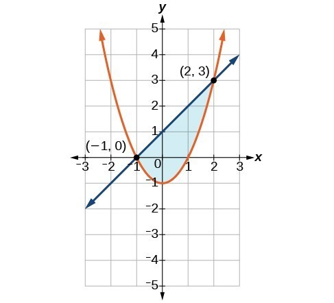
1. A nonlinear system could be representative of two circles that overlap and intersect in two locations, hence two solutions. A nonlinear system could be representative of a parabola and a circle, where the vertex of the parabola meets the circle and the branches also intersect the circle, hence three solutions.
3. No. There does not need to be a feasible region. Consider a system that is bounded by two parallel lines. One inequality represents the region above the upper line; the other represents the region below the lower line. In this case, no points in the plane are located in both regions; hence there is no feasible region.
5. Choose any number between each solution and plug into [latex]C\left(x\right)[/latex] and [latex]R\left(x\right)[/latex]. If [latex]C\left(x\right)<R\left(x\right),\text{}[/latex] then there is profit.
7. [latex]\left(0,-3\right),\left(3,0\right)[/latex]
9. [latex]\left(-\frac{3\sqrt{2}}{2},\frac{3\sqrt{2}}{2}\right),\left(\frac{3\sqrt{2}}{2},-\frac{3\sqrt{2}}{2}\right)[/latex]
11. [latex]\left(-3,0\right),\left(3,0\right)[/latex]
13. [latex]\left(\frac{1}{4},-\frac{\sqrt{62}}{8}\right),\left(\frac{1}{4},\frac{\sqrt{62}}{8}\right)[/latex]
15. [latex]\left(-\frac{\sqrt{398}}{4},\frac{199}{4}\right),\left(\frac{\sqrt{398}}{4},\frac{199}{4}\right)[/latex]
17. [latex]\left(0,2\right),\left(1,3\right)[/latex]
19. [latex]\left(-\sqrt{\frac{1}{2}\left(\sqrt{5}-1\right)},\frac{1}{2}\left(1-\sqrt{5}\right)\right),\left(\sqrt{\frac{1}{2}\left(\sqrt{5}-1\right)},\frac{1}{2}\left(1-\sqrt{5}\right)\right)[/latex]
21. [latex]\left(5,0\right)[/latex]
23. [latex]\left(0,0\right)[/latex]
25. [latex]\left(3,0\right)[/latex]
27. No Solutions Exist
29. No Solutions Exist
31. [latex]\left(-\frac{\sqrt{2}}{2},-\frac{\sqrt{2}}{2}\right),\left(-\frac{\sqrt{2}}{2},\frac{\sqrt{2}}{2}\right),\left(\frac{\sqrt{2}}{2},-\frac{\sqrt{2}}{2}\right),\left(\frac{\sqrt{2}}{2},\frac{\sqrt{2}}{2}\right)[/latex]
33. [latex]\left(2,0\right)[/latex]
35. [latex]\left(-\sqrt{7},-3\right),\left(-\sqrt{7},3\right),\left(\sqrt{7},-3\right),\left(\sqrt{7},3\right)[/latex]
37. [latex]\left(-\sqrt{\frac{1}{2}\left(\sqrt{73}-5\right)},\frac{1}{2}\left(7-\sqrt{73}\right)\right),\left(\sqrt{\frac{1}{2}\left(\sqrt{73}-5\right)},\frac{1}{2}\left(7-\sqrt{73}\right)\right)[/latex]
39.
41.
43.
45.
47.
49. [latex]\left(-2\sqrt{\frac{70}{383}},-2\sqrt{\frac{35}{29}}\right),\left(-2\sqrt{\frac{70}{383}},2\sqrt{\frac{35}{29}}\right),\left(2\sqrt{\frac{70}{383}},-2\sqrt{\frac{35}{29}}\right),\left(2\sqrt{\frac{70}{383}},2\sqrt{\frac{35}{29}}\right)[/latex]
51. No Solution Exists
53. [latex]x=0,y>0[/latex] and [latex]0<x<1,\sqrt{x}<y<\frac{1}{x}[/latex]
55. 12, 288
57. 2–20 computers
By the end of this section, you will be able to:

Figure 1. (credit: “SD Dirk,” Flickr)
Two club soccer teams, the Wildcats and the Mud Cats, are hoping to obtain new equipment for an upcoming season. [link] shows the needs of both teams.
| Wildcats | Mud Cats | |
|---|---|---|
| Goals | 6 | 10 |
| Balls | 30 | 24 |
| Jerseys | 14 | 20 |
A goal costs $300; a ball costs $10; and a jersey costs $30. How can we find the total cost for the equipment needed for each team? In this section, we discover a method in which the data in the soccer equipment table can be displayed and used for calculating other information. Then, we will be able to calculate the cost of the equipment.
To solve a problem like the one described for the soccer teams, we can use a matrix, which is a rectangular array of numbers. A row in a matrix is a set of numbers that are aligned horizontally. A column in a matrix is a set of numbers that are aligned vertically. Each number is an entry, sometimes called an element, of the matrix. Matrices (plural) are enclosed in [ ] or ( ), and are usually named with capital letters. For example, three matrices named [latex]A,B,\text{}[/latex] and [latex]C[/latex] are shown below.
A matrix is often referred to by its size or dimensions: [latex]\text{ }m\text{ }\times \text{ }n\text{ }[/latex] indicating [latex]m[/latex] rows and [latex]n[/latex] columns. Matrix entries are defined first by row and then by column. For example, to locate the entry in matrix [latex]A[/latex] identified as [latex]{a}_{ij},\text{}[/latex] we look for the entry in row [latex]i,\text{}[/latex] column [latex]j[/latex]. In matrix [latex]A\text{, \hspace{0.17em}}[/latex] shown below, the entry in row 2, column 3 is [latex]{a}_{23}[/latex].
A square matrix is a matrix with dimensions [latex]\text{ }n\text{ }\times \text{ }n,\text{}[/latex] meaning that it has the same number of rows as columns. The [latex]3\times 3[/latex] matrix above is an example of a square matrix.
A row matrix is a matrix consisting of one row with dimensions [latex]1\text{ }\times \text{ }n[/latex].
A column matrix is a matrix consisting of one column with dimensions [latex]m\text{ }\times \text{ }1[/latex].
A matrix may be used to represent a system of equations. In these cases, the numbers represent the coefficients of the variables in the system. Matrices often make solving systems of equations easier because they are not encumbered with variables. We will investigate this idea further in the next section, but first we will look at basic matrix operations.
A matrix is a rectangular array of numbers that is usually named by a capital letter: [latex]A,B,C,\text{}[/latex] and so on. Each entry in a matrix is referred to as [latex]{a}_{ij}[/latex], such that [latex]i[/latex] represents the row and [latex]j[/latex] represents the column. Matrices are often referred to by their dimensions: [latex]m\times n[/latex] indicating [latex]m[/latex] rows and [latex]n[/latex] columns.
Given matrix [latex]A:[/latex]
We use matrices to list data or to represent systems. Because the entries are numbers, we can perform operations on matrices. We add or subtract matrices by adding or subtracting corresponding entries.
In order to do this, the entries must correspond. Therefore, addition and subtraction of matrices is only possible when the matrices have the same dimensions. We can add or subtract a [latex]\text{ }3\text{ }\times \text{ }3\text{ }[/latex] matrix and another [latex]\text{ }3\text{ }\times \text{ }3\text{ }[/latex] matrix, but we cannot add or subtract a [latex]\text{ }2\text{ }\times \text{ }3\text{ }[/latex] matrix and a [latex]\text{ }3\text{ }\times \text{ }3\text{ }[/latex] matrix because some entries in one matrix will not have a corresponding entry in the other matrix.
Given matrices [latex]A[/latex] and [latex]B[/latex] of like dimensions, addition and subtraction of [latex]A[/latex] and [latex]B[/latex] will produce matrix [latex]C[/latex] or matrix [latex]D[/latex] of the same dimension.
Matrix addition is commutative.
It is also associative.
Find the sum of [latex]A[/latex] and [latex]B,\text{}[/latex] given
Add corresponding entries.
Find the sum of [latex]A[/latex] and [latex]B[/latex].
Add corresponding entries. Add the entry in row 1, column 1, [latex]{a}_{11},\text{}[/latex] of matrix [latex]A[/latex] to the entry in row 1, column 1, [latex]{b}_{11}[/latex], of [latex]B[/latex]. Continue the pattern until all entries have been added.
Find the difference of [latex]A[/latex] and [latex]B[/latex].
We subtract the corresponding entries of each matrix.
Given [latex]A[/latex] and [latex]B:[/latex]
Add matrix [latex]A[/latex] and matrix [latex]B[/latex].
Besides adding and subtracting whole matrices, there are many situations in which we need to multiply a matrix by a constant called a scalar. Recall that a scalar is a real number quantity that has magnitude, but not direction. For example, time, temperature, and distance are scalar quantities. The process of scalar multiplication involves multiplying each entry in a matrix by a scalar. A scalar multiple is any entry of a matrix that results from scalar multiplication.
Consider a real-world scenario in which a university needs to add to its inventory of computers, computer tables, and chairs in two of the campus labs due to increased enrollment. They estimate that 15% more equipment is needed in both labs. The school’s current inventory is displayed in the table below.
| Lab A | Lab B | |
|---|---|---|
| Computers | 15 | 27 |
| Computer Tables | 16 | 34 |
| Chairs | 16 | 34 |
Converting the data to a matrix, we have
To calculate how much computer equipment will be needed, we multiply all entries in matrix [latex]C[/latex] by 0.15.
We must round up to the next integer, so the amount of new equipment needed is
Adding the two matrices as shown below, we see the new inventory amounts.
This means
Thus, Lab A will have 18 computers, 19 computer tables, and 19 chairs; Lab B will have 32 computers, 40 computer tables, and 40 chairs.
Scalar multiplication involves finding the product of a constant by each entry in the matrix. Given
the scalar multiple [latex]cA[/latex] is
Scalar multiplication is distributive. For the matrices [latex]A,B[/latex], and [latex]C[/latex] with scalars [latex]a[/latex] and [latex]b[/latex],
Multiply matrix [latex]A[/latex] by the scalar 3.
Multiply each entry in [latex]A[/latex] by the scalar 3.
Given matrix [latex]B,\text{}[/latex] find [latex]-2B[/latex] where
Find the sum [latex]3A+2B[/latex].
First, find [latex]3A,\text{}[/latex] then [latex]2B[/latex].
Now, add [latex]3A+2B[/latex].
In addition to multiplying a matrix by a scalar, we can multiply two matrices. Finding the product of two matrices is only possible when the inner dimensions are the same, meaning that the number of columns of the first matrix is equal to the number of rows of the second matrix. If [latex]A[/latex] is an [latex]\text{ }m\text{ }\times \text{ }r\text{ }[/latex] matrix and [latex]B[/latex] is an [latex]\text{ }r\text{ }\times \text{ }n\text{ }[/latex] matrix, then the product matrix [latex]AB[/latex] is an [latex]\text{ }m\text{ }\times \text{ }n\text{ }[/latex] matrix. For example, the product [latex]AB[/latex] is possible because the number of columns in [latex]A[/latex] is the same as the number of rows in [latex]B[/latex]. If the inner dimensions do not match, the product is not defined.
Figure 1
We multiply entries of [latex]A[/latex] with entries of [latex]B[/latex] according to a specific pattern as outlined below. The process of matrix multiplication becomes clearer when working a problem with real numbers.
To obtain the entries in row [latex]i[/latex] of [latex]AB,\text{}[/latex] we multiply the entries in row [latex]i[/latex] of [latex]A[/latex] by column [latex]j[/latex] in [latex]B[/latex] and add. For example, given matrices [latex]A[/latex] and [latex]B,\text{}[/latex] where the dimensions of [latex]A[/latex] are [latex]2\text{ }\times \text{ }3[/latex] and the dimensions of [latex]B[/latex] are [latex]3\text{ }\times \text{ }3,\text{}[/latex] the product of [latex]AB[/latex] will be a [latex]2\text{ }\times \text{ }3[/latex] matrix.
Multiply and add as follows to obtain the first entry of the product matrix [latex]AB[/latex].
We proceed the same way to obtain the second row of [latex]AB[/latex]. In other words, row 2 of [latex]A[/latex] times column 1 of [latex]B[/latex]; row 2 of [latex]A[/latex] times column 2 of [latex]B[/latex]; row 2 of [latex]A[/latex] times column 3 of [latex]B[/latex]. When complete, the product matrix will be
For the matrices [latex]A,B,\text{}[/latex] and [latex]C[/latex] the following properties hold.
Note that matrix multiplication is not commutative.
Multiply matrix [latex]A[/latex] and matrix [latex]B[/latex].
First, we check the dimensions of the matrices. Matrix [latex]A[/latex] has dimensions [latex]2\times 2[/latex] and matrix [latex]B[/latex] has dimensions [latex]2\times 2[/latex]. The inner dimensions are the same so we can perform the multiplication. The product will have the dimensions [latex]2\times 2[/latex].
We perform the operations outlined previously.
Figure 2
Given [latex]A[/latex] and [latex]B:[/latex]
Notice that the products [latex]AB[/latex] and [latex]BA[/latex] are not equal.
This illustrates the fact that matrix multiplication is not commutative.
Yes, consider a matrix A with dimension [latex]3\times 4[/latex] and matrix B with dimension [latex]4\times 2[/latex]. For the product AB the inner dimensions are 4 and the product is defined, but for the product BA the inner dimensions are 2 and 3 so the product is undefined.
Let’s return to the problem presented at the opening of this section. We have the table below, representing the equipment needs of two soccer teams.
| Wildcats | Mud Cats | |
|---|---|---|
| Goals | 6 | 10 |
| Balls | 30 | 24 |
| Jerseys | 14 | 20 |
We are also given the prices of the equipment, as shown in the table below.
| Goal | $300 |
| Ball | $10 |
| Jersey | $30 |
We will convert the data to matrices. Thus, the equipment need matrix is written as
The cost matrix is written as
We perform matrix multiplication to obtain costs for the equipment.
The total cost for equipment for the Wildcats is $2,520, and the total cost for equipment for the Mud Cats is $3,840.
Find [latex]AB-C[/latex] given
On the matrix page of the calculator, we enter matrix [latex]A[/latex] above as the matrix variable [latex]\left[A\right][/latex], matrix [latex]B[/latex] above as the matrix variable [latex]\left[B\right][/latex], and matrix [latex]C[/latex] above as the matrix variable [latex]\left[C\right][/latex].
On the home screen of the calculator, we type in the problem and call up each matrix variable as needed.
The calculator gives us the following matrix.
1. Can we add any two matrices together? If so, explain why; if not, explain why not and give an example of two matrices that cannot be added together.
2. Can we multiply any column matrix by any row matrix? Explain why or why not.
3. Can both the products [latex]AB[/latex] and [latex]BA[/latex] be defined? If so, explain how; if not, explain why.
4. Can any two matrices of the same size be multiplied? If so, explain why, and if not, explain why not and give an example of two matrices of the same size that cannot be multiplied together.
5. Does matrix multiplication commute? That is, does [latex]AB=BA?[/latex] If so, prove why it does. If not, explain why it does not.
For the following exercises, use the matrices below and perform the matrix addition or subtraction. Indicate if the operation is undefined.
[latex]A=\left[\begin{array}{cc}1& 3\\ 0& 7\end{array}\right],B=\left[\begin{array}{cc}2& 14\\ 22& 6\end{array}\right],C=\left[\begin{array}{cc}1& 5\\ 8& 92\\ 12& 6\end{array}\right],D=\left[\begin{array}{cc}10& 14\\ 7& 2\\ 5& 61\end{array}\right],E=\left[\begin{array}{cc}6& 12\\ 14& 5\end{array}\right],F=\left[\begin{array}{cc}0& 9\\ 78& 17\\ 15& 4\end{array}\right][/latex]
6. [latex]A+B[/latex]
7. [latex]C+D[/latex]
8. [latex]A+C[/latex]
9. [latex]B-E[/latex]
10. [latex]C+F[/latex]
11. [latex]D-B[/latex]
For the following exercises, use the matrices below to perform scalar multiplication.
[latex]A=\left[\begin{array}{rr}\hfill 4& \hfill 6\\ \hfill 13& \hfill 12\end{array}\right],B=\left[\begin{array}{rr}\hfill 3& \hfill 9\\ \hfill 21& \hfill 12\\ \hfill 0& \hfill 64\end{array}\right],C=\left[\begin{array}{rrrr}\hfill 16& \hfill 3& \hfill 7& \hfill 18\\ \hfill 90& \hfill 5& \hfill 3& \hfill 29\end{array}\right],D=\left[\begin{array}{rrr}\hfill 18& \hfill 12& \hfill 13\\ \hfill 8& \hfill 14& \hfill 6\\ \hfill 7& \hfill 4& \hfill 21\end{array}\right][/latex]
12. [latex]5A[/latex]
13. [latex]3B[/latex]
14. [latex]-2B[/latex]
15. [latex]-4C[/latex]
16. [latex]\frac{1}{2}C[/latex]
17. [latex]100D[/latex]
For the following exercises, use the matrices below to perform matrix multiplication.
[latex]A=\left[\begin{array}{rr}\hfill -1& \hfill 5\\ \hfill 3& \hfill 2\end{array}\right],B=\left[\begin{array}{rrr}\hfill 3& \hfill 6& \hfill 4\\ \hfill -8& \hfill 0& \hfill 12\end{array}\right],C=\left[\begin{array}{rr}\hfill 4& \hfill 10\\ \hfill -2& \hfill 6\\ \hfill 5& \hfill 9\end{array}\right],D=\left[\begin{array}{rrr}\hfill 2& \hfill -3& \hfill 12\\ \hfill 9& \hfill 3& \hfill 1\\ \hfill 0& \hfill 8& \hfill -10\end{array}\right][/latex]
18. [latex]AB[/latex]
19. [latex]BC[/latex]
20. [latex]CA[/latex]
21. [latex]BD[/latex]
22. [latex]DC[/latex]
23. [latex]CB[/latex]
For the following exercises, use the matrices below to perform the indicated operation if possible. If not possible, explain why the operation cannot be performed.
[latex]A=\left[\begin{array}{rr}\hfill 2& \hfill -5\\ \hfill 6& \hfill 7\end{array}\right],B=\left[\begin{array}{rr}\hfill -9& \hfill 6\\ \hfill -4& \hfill 2\end{array}\right],C=\left[\begin{array}{rr}\hfill 0& \hfill 9\\ \hfill 7& \hfill 1\end{array}\right],D=\left[\begin{array}{rrr}\hfill -8& \hfill 7& \hfill -5\\ \hfill 4& \hfill 3& \hfill 2\\ \hfill 0& \hfill 9& \hfill 2\end{array}\right],E=\left[\begin{array}{rrr}\hfill 4& \hfill 5& \hfill 3\\ \hfill 7& \hfill -6& \hfill -5\\ \hfill 1& \hfill 0& \hfill 9\end{array}\right][/latex]
24. [latex]A+B-C[/latex]
25. [latex]4A+5D[/latex]
26. [latex]2C+B[/latex]
27. [latex]3D+4E[/latex]
28. [latex]C - 0.5D[/latex]
29. [latex]100D - 10E[/latex]
For the following exercises, use the matrices below to perform the indicated operation if possible. If not possible, explain why the operation cannot be performed. (Hint: [latex]{A}^{2}=A\cdot A[/latex])
[latex]A=\left[\begin{array}{rr}\hfill -10& \hfill 20\\ \hfill 5& \hfill 25\end{array}\right],B=\left[\begin{array}{rr}\hfill 40& \hfill 10\\ \hfill -20& \hfill 30\end{array}\right],C=\left[\begin{array}{rr}\hfill -1& \hfill 0\\ \hfill 0& \hfill -1\\ \hfill 1& \hfill 0\end{array}\right][/latex]
30. [latex]AB[/latex]
31. [latex]BA[/latex]
32. [latex]CA[/latex]
33. [latex]BC[/latex]
34. [latex]{A}^{2}[/latex]
35. [latex]{B}^{2}[/latex]
36. [latex]{C}^{2}[/latex]
37. [latex]{B}^{2}{A}^{2}[/latex]
38. [latex]{A}^{2}{B}^{2}[/latex]
39. [latex]{\left(AB\right)}^{2}[/latex]
40. [latex]{\left(BA\right)}^{2}[/latex]
For the following exercises, use the matrices below to perform the indicated operation if possible. If not possible, explain why the operation cannot be performed. (Hint: [latex]{A}^{2}=A\cdot A[/latex])
[latex]A=\left[\begin{array}{rr}\hfill 1& \hfill 0\\ \hfill 2& \hfill 3\end{array}\right],B=\left[\begin{array}{rrr}\hfill -2& \hfill 3& \hfill 4\\ \hfill -1& \hfill 1& \hfill -5\end{array}\right],C=\left[\begin{array}{rr}\hfill 0.5& \hfill 0.1\\ \hfill 1& \hfill 0.2\\ \hfill -0.5& \hfill 0.3\end{array}\right],D=\left[\begin{array}{rrr}\hfill 1& \hfill 0& \hfill -1\\ \hfill -6& \hfill 7& \hfill 5\\ \hfill 4& \hfill 2& \hfill 1\end{array}\right][/latex]
41. [latex]AB[/latex]
42. [latex]BA[/latex]
43. [latex]BD[/latex]
44. [latex]DC[/latex]
45. [latex]{D}^{2}[/latex]
46. [latex]{A}^{2}[/latex]
47. [latex]{D}^{3}[/latex]
48. [latex]\left(AB\right)C[/latex]
49. [latex]A\left(BC\right)[/latex]
For the following exercises, use the matrices below to perform the indicated operation if possible. If not possible, explain why the operation cannot be performed. Use a calculator to verify your solution.
[latex]A=\left[\begin{array}{rrr}\hfill -2& \hfill 0& \hfill 9\\ \hfill 1& \hfill 8& \hfill -3\\ \hfill 0.5& \hfill 4& \hfill 5\end{array}\right],B=\left[\begin{array}{rrr}\hfill 0.5& \hfill 3& \hfill 0\\ \hfill -4& \hfill 1& \hfill 6\\ \hfill 8& \hfill 7& \hfill 2\end{array}\right],C=\left[\begin{array}{rrr}\hfill 1& \hfill 0& \hfill 1\\ \hfill 0& \hfill 1& \hfill 0\\ \hfill 1& \hfill 0& \hfill 1\end{array}\right][/latex]
50. [latex]AB[/latex]
51. [latex]BA[/latex]
52. [latex]CA[/latex]
53. [latex]BC[/latex]
54. [latex]ABC[/latex]
For the following exercises, use the matrix below to perform the indicated operation on the given matrix.
[latex]B=\left[\begin{array}{rrr}\hfill 1& \hfill 0& \hfill 0\\ \hfill 0& \hfill 0& \hfill 1\\ \hfill 0& \hfill 1& \hfill 0\end{array}\right][/latex]
55. [latex]{B}^{2}[/latex]
56. [latex]{B}^{3}[/latex]
57. [latex]{B}^{4}[/latex]
58. [latex]{B}^{5}[/latex]
59. Using the above questions, find a formula for [latex]{B}^{n}[/latex]. Test the formula for [latex]{B}^{201}[/latex] and [latex]{B}^{202},\text{}[/latex] using a calculator.
1. [latex]A+B=\left[\begin{array}{c}2\\ 1\\ 1\end{array}\begin{array}{c}6\\ \text{ }\text{ }\text{ }0\\ -3\end{array}\right]+\left[\begin{array}{c}3\\ 1\\ -4\end{array}\begin{array}{c}-2\\ 5\\ 3\end{array}\right]=\left[\begin{array}{c}2+3\\ 1+1\\ 1+\left(-4\right)\end{array}\begin{array}{c}6+\left(-2\right)\\ 0+5\\ -3+3\end{array}\right]=\left[\begin{array}{c}5\\ 2\\ -3\end{array}\begin{array}{c}4\\ 5\\ 0\end{array}\right][/latex]
2. [latex]-2B=\left[\begin{array}{cc}-8& -2\\ -6& -4\end{array}\right][/latex]
1. No, they must have the same dimensions. An example would include two matrices of different dimensions. One cannot add the following two matrices because the first is a [latex]2\times 2[/latex] matrix and the second is a [latex]2\times 3[/latex] matrix. [latex]\left[\begin{array}{cc}1& 2\\ 3& 4\end{array}\right]+\left[\begin{array}{ccc}6& 5& 4\\ 3& 2& 1\end{array}\right][/latex] has no sum.
3. Yes, if the dimensions of [latex]A[/latex] are [latex]m\times n[/latex] and the dimensions of [latex]B[/latex] are [latex]n\times m,\text{}[/latex] both products will be defined.
5. Not necessarily. To find [latex]AB,\text{}[/latex] we multiply the first row of [latex]A[/latex] by the first column of [latex]B[/latex] to get the first entry of [latex]AB[/latex]. To find [latex]BA,\text{}[/latex] we multiply the first row of [latex]B[/latex] by the first column of [latex]A[/latex] to get the first entry of [latex]BA[/latex]. Thus, if those are unequal, then the matrix multiplication does not commute.
7. [latex]\left[\begin{array}{cc}11& 19\\ 15& 94\\ 17& 67\end{array}\right][/latex]
9. [latex]\left[\begin{array}{cc}-4& 2\\ 8& 1\end{array}\right][/latex]
11. Undidentified; dimensions do not match
13. [latex]\left[\begin{array}{cc}9& 27\\ 63& 36\\ 0& 192\end{array}\right][/latex]
15. [latex]\left[\begin{array}{cccc}-64& -12& -28& -72\\ -360& -20& -12& -116\end{array}\right][/latex]
17. [latex]\left[\begin{array}{ccc}1,800& 1,200& 1,300\\ 800& 1,400& 600\\ 700& 400& 2,100\end{array}\right][/latex]
19. [latex]\left[\begin{array}{cc}20& 102\\ 28& 28\end{array}\right][/latex]
21. [latex]\left[\begin{array}{ccc}60& 41& 2\\ -16& 120& -216\end{array}\right][/latex]
23. [latex]\left[\begin{array}{ccc}-68& 24& 136\\ -54& -12& 64\\ -57& 30& 128\end{array}\right][/latex]
25. Undefined; dimensions do not match.
27. [latex]\left[\begin{array}{ccc}-8& 41& -3\\ 40& -15& -14\\ 4& 27& 42\end{array}\right][/latex]
29. [latex]\left[\begin{array}{ccc}-840& 650& -530\\ 330& 360& 250\\ -10& 900& 110\end{array}\right][/latex]
31. [latex]\left[\begin{array}{cc}-350& 1,050\\ 350& 350\end{array}\right][/latex]
33. Undefined; inner dimensions do not match.
35. [latex]\left[\begin{array}{cc}1,400& 700\\ -1,400& 700\end{array}\right][/latex]
37. [latex]\left[\begin{array}{cc}332,500& 927,500\\ -227,500& 87,500\end{array}\right][/latex]
39. [latex]\left[\begin{array}{cc}490,000& 0\\ 0& 490,000\end{array}\right][/latex]
41. [latex]\left[\begin{array}{ccc}-2& 3& 4\\ -7& 9& -7\end{array}\right][/latex]
43. [latex]\left[\begin{array}{ccc}-4& 29& 21\\ -27& -3& 1\end{array}\right][/latex]
45. [latex]\left[\begin{array}{ccc}-3& -2& -2\\ -28& 59& 46\\ -4& 16& 7\end{array}\right][/latex]
47. [latex]\left[\begin{array}{ccc}1& -18& -9\\ -198& 505& 369\\ -72& 126& 91\end{array}\right][/latex]
49. [latex]\left[\begin{array}{cc}0& 1.6\\ 9& -1\end{array}\right][/latex]
51. [latex]\left[\begin{array}{ccc}2& 24& -4.5\\ 12& 32& -9\\ -8& 64& 61\end{array}\right][/latex]
53. [latex]\left[\begin{array}{ccc}0.5& 3& 0.5\\ 2& 1& 2\\ 10& 7& 10\end{array}\right][/latex]
55. [latex]\left[\begin{array}{ccc}1& 0& 0\\ 0& 1& 0\\ 0& 0& 1\end{array}\right][/latex]
57. [latex]\left[\begin{array}{ccc}1& 0& 0\\ 0& 1& 0\\ 0& 0& 1\end{array}\right][/latex]
59. [latex]{B}^{n}=\left\{\begin{array}{l}\left[\begin{array}{ccc}1& 0& 0\\ 0& 1& 0\\ 0& 0& 1\end{array}\right],\text{ }n\text{even,}\\ \left[\begin{array}{ccc}1& 0& 0\\ 0& 0& 1\\ 0& 1& 0\end{array}\right],\text{ }n\text{odd}\text{.}\end{array}[/latex]
By the end of this section, you will be able to:
Figure 1. German mathematician Carl Friedrich Gauss (1777–1855).
Carl Friedrich Gauss lived during the late 18th century and early 19th century, but he is still considered one of the most prolific mathematicians in history. His contributions to the science of mathematics and physics span fields such as algebra, number theory, analysis, differential geometry, astronomy, and optics, among others. His discoveries regarding matrix theory changed the way mathematicians have worked for the last two centuries.
We first encountered Gaussian elimination in Systems of Linear Equations: Two Variables. In this section, we will revisit this technique for solving systems, this time using matrices.
A matrix can serve as a device for representing and solving a system of equations. To express a system in matrix form, we extract the coefficients of the variables and the constants, and these become the entries of the matrix. We use a vertical line to separate the coefficient entries from the constants, essentially replacing the equal signs. When a system is written in this form, we call it an augmented matrix.
For example, consider the following [latex]2\times 2[/latex] system of equations.
We can write this system as an augmented matrix:
We can also write a matrix containing just the coefficients. This is called the coefficient matrix.
A three-by-three system of equations such as
has a coefficient matrix
and is represented by the augmented matrix
Notice that the matrix is written so that the variables line up in their own columns: x-terms go in the first column, y-terms in the second column, and z-terms in the third column. It is very important that each equation is written in standard form [latex]ax+by+cz=d[/latex] so that the variables line up. When there is a missing variable term in an equation, the coefficient is 0.
Write the augmented matrix for the given system of equations.
The augmented matrix displays the coefficients of the variables, and an additional column for the constants.
Write the augmented matrix of the given system of equations.
We can use augmented matrices to help us solve systems of equations because they simplify operations when the systems are not encumbered by the variables. However, it is important to understand how to move back and forth between formats in order to make finding solutions smoother and more intuitive. Here, we will use the information in an augmented matrix to write the system of equations in standard form.
Find the system of equations from the augmented matrix.
When the columns represent the variables [latex]x[/latex], [latex]y[/latex], and [latex]z[/latex],
Write the system of equations from the augmented matrix.
Now that we can write systems of equations in augmented matrix form, we will examine the various row operations that can be performed on a matrix, such as addition, multiplication by a constant, and interchanging rows.
Performing row operations on a matrix is the method we use for solving a system of equations. In order to solve the system of equations, we want to convert the matrix to row-echelon form, in which there are ones down the main diagonal from the upper left corner to the lower right corner, and zeros in every position below the main diagonal as shown.
We use row operations corresponding to equation operations to obtain a new matrix that is row-equivalent in a simpler form. Here are the guidelines to obtaining row-echelon form.
To solve a system of equations we can perform the following row operations to convert the coefficient matrix to row-echelon form and do back-substitution to find the solution.
Each of the row operations corresponds to the operations we have already learned to solve systems of equations in three variables. With these operations, there are some key moves that will quickly achieve the goal of writing a matrix in row-echelon form. To obtain a matrix in row-echelon form for finding solutions, we use Gaussian elimination, a method that uses row operations to obtain a 1 as the first entry so that row 1 can be used to convert the remaining rows.
The Gaussian elimination method refers to a strategy used to obtain the row-echelon form of a matrix. The goal is to write matrix [latex]A[/latex] with the number 1 as the entry down the main diagonal and have all zeros below.
The first step of the Gaussian strategy includes obtaining a 1 as the first entry, so that row 1 may be used to alter the rows below.
Solve the given system by Gaussian elimination.
First, we write this as an augmented matrix.
We want a 1 in row 1, column 1. This can be accomplished by interchanging row 1 and row 2.
We now have a 1 as the first entry in row 1, column 1. Now let’s obtain a 0 in row 2, column 1. This can be accomplished by multiplying row 1 by [latex]-2[/latex], and then adding the result to row 2.
We only have one more step, to multiply row 2 by [latex]\frac{1}{5}[/latex].
Use back-substitution. The second row of the matrix represents [latex]y=1[/latex]. Back-substitute [latex]y=1[/latex] into the first equation.
The solution is the point [latex]\left(\frac{3}{2},1\right)[/latex].
Solve the given system by Gaussian elimination.
Use Gaussian elimination to solve the given [latex]2\times 2[/latex] system of equations.
Write the system as an augmented matrix.
Obtain a 1 in row 1, column 1. This can be accomplished by multiplying the first row by [latex]\frac{1}{2}[/latex].
Next, we want a 0 in row 2, column 1. Multiply row 1 by [latex]-4[/latex] and add row 1 to row 2.
The second row represents the equation [latex]0=4[/latex]. Therefore, the system is inconsistent and has no solution.
Solve the system of equations.
Perform row operations on the augmented matrix to try and achieve row-echelon form.
The matrix ends up with all zeros in the last row: [latex]0y=0[/latex]. Thus, there are an infinite number of solutions and the system is classified as dependent. To find the generic solution, return to one of the original equations and solve for [latex]y[/latex].
So the solution to this system is [latex]\left(x,3-\frac{3}{4}x\right)[/latex].
Perform row operations on the given matrix to obtain row-echelon form.
The first row already has a 1 in row 1, column 1. The next step is to multiply row 1 by [latex]-2[/latex] and add it to row 2. Then replace row 2 with the result.
Next, obtain a zero in row 3, column 1.
Next, obtain a zero in row 3, column 2.
The last step is to obtain a 1 in row 3, column 3.
Write the system of equations in row-echelon form.
We have seen how to write a system of equations with an augmented matrix, and then how to use row operations and back-substitution to obtain row-echelon form. Now, we will take row-echelon form a step farther to solve a 3 by 3 system of linear equations. The general idea is to eliminate all but one variable using row operations and then back-substitute to solve for the other variables.
Solve the system of linear equations using matrices.
First, we write the augmented matrix.
Next, we perform row operations to obtain row-echelon form.
The easiest way to obtain a 1 in row 2 of column 1 is to interchange [latex]{R}_{2}[/latex] and [latex]{R}_{3}[/latex].
Then
The last matrix represents the equivalent system.
Using back-substitution, we obtain the solution as [latex]\left(4,-3,1\right)[/latex].
Solve the following system of linear equations using matrices.
Write the augmented matrix.
First, multiply row 1 by [latex]-1[/latex] to get a 1 in row 1, column 1. Then, perform row operations to obtain row-echelon form.
The last matrix represents the following system.
We see by the identity [latex]0=0[/latex] that this is a dependent system with an infinite number of solutions. We then find the generic solution. By solving the second equation for [latex]y[/latex] and substituting it into the first equation we can solve for [latex]z[/latex] in terms of [latex]x[/latex].
Now we substitute the expression for [latex]z[/latex] into the second equation to solve for [latex]y[/latex] in terms of [latex]x[/latex].
The generic solution is [latex]\left(x,\frac{2 - 2x}{3},\frac{1-x}{3}\right)[/latex].
Solve the system using matrices.
Yes, a system of linear equations of any size can be solved by Gaussian elimination.
Solve the system of equations.
Write the augmented matrix for the system of equations.
On the matrix page of the calculator, enter the augmented matrix above as the matrix variable [latex]\left[A\right][/latex].
Use the ref( function in the calculator, calling up the matrix variable [latex]\left[A\right][/latex].
Evaluate.
Using back-substitution, the solution is [latex]\left(\frac{61}{187},-\frac{92}{187},-\frac{24}{187}\right)[/latex].
Carolyn invests a total of $12,000 in two municipal bonds, one paying 10.5% interest and the other paying 12% interest. The annual interest earned on the two investments last year was $1,335. How much was invested at each rate?
We have a system of two equations in two variables. Let [latex]x=[/latex] the amount invested at 10.5% interest, and [latex]y=[/latex] the amount invested at 12% interest.
As a matrix, we have
Multiply row 1 by [latex]-0.105[/latex] and add the result to row 2.
Then,
So [latex]12,000 - 5,000=7,000[/latex].
Thus, $5,000 was invested at 12% interest and $7,000 at 10.5% interest.
Ava invests a total of $10,000 in three accounts, one paying 5% interest, another paying 8% interest, and the third paying 9% interest. The annual interest earned on the three investments last year was $770. The amount invested at 9% was twice the amount invested at 5%. How much was invested at each rate?
We have a system of three equations in three variables. Let [latex]x[/latex] be the amount invested at 5% interest, let [latex]y[/latex] be the amount invested at 8% interest, and let [latex]z[/latex] be the amount invested at 9% interest. Thus,
As a matrix, we have
Now, we perform Gaussian elimination to achieve row-echelon form.
The third row tells us [latex]-\frac{1}{3}z=-2,000[/latex]; thus [latex]z=6,000[/latex].
The second row tells us [latex]y+\frac{4}{3}z=9,000[/latex]. Substituting [latex]z=6,000[/latex], we get
The first row tells us [latex]x+y+z=10,000[/latex]. Substituting [latex]y=1,000[/latex] and [latex]z=6,000[/latex], we get
The answer is $3,000 invested at 5% interest, $1,000 invested at 8%, and $6,000 invested at 9% interest.
A small shoe company took out a loan of $1,500,000 to expand their inventory. Part of the money was borrowed at 7%, part was borrowed at 8%, and part was borrowed at 10%. The amount borrowed at 10% was four times the amount borrowed at 7%, and the annual interest on all three loans was $130,500. Use matrices to find the amount borrowed at each rate.
1. Can any system of linear equations be written as an augmented matrix? Explain why or why not. Explain how to write that augmented matrix.
2. Can any matrix be written as a system of linear equations? Explain why or why not. Explain how to write that system of equations.
3. Is there only one correct method of using row operations on a matrix? Try to explain two different row operations possible to solve the augmented matrix [latex]\left[\begin{array}{rr}\hfill 9& \hfill 3\\ \hfill 1& \hfill -2\end{array}\text{ }|\text{ }\begin{array}{r}\hfill 0\\ \hfill 6\end{array}\right][/latex].
4. Can a matrix whose entry is 0 on the diagonal be solved? Explain why or why not. What would you do to remedy the situation?
5. Can a matrix that has 0 entries for an entire row have one solution? Explain why or why not.
For the following exercises, write the augmented matrix for the linear system.
6. [latex]\begin{array}{l}8x - 37y=8\\ 2x+12y=3\end{array}[/latex]
7. [latex]\begin{array}{l}\text{ }16y=4\hfill \\ 9x-y=2\hfill \end{array}[/latex]
8. [latex]\begin{array}{l}\text{ }3x+2y+10z=3\hfill \\ -6x+2y+5z=13\hfill \\ \text{ }4x+z=18\hfill \end{array}[/latex]
9. [latex]\begin{array}{l}\hfill \\ \text{ }x+5y+8z=19\hfill \\ \text{ }12x+3y=4\hfill \\ 3x+4y+9z=-7\hfill \end{array}[/latex]
10. [latex]\begin{array}{l}6x+12y+16z=4\hfill \\ \text{ }19x - 5y+3z=-9\hfill \\ \text{ }x+2y=-8\hfill \end{array}[/latex]
For the following exercises, write the linear system from the augmented matrix.
11. [latex]\left[\begin{array}{rr}\hfill -2& \hfill 5\\ \hfill 6& \hfill -18\end{array}\text{ }|\text{ }\begin{array}{r}\hfill 5\\ \hfill 26\end{array}\right][/latex]
12. [latex]\left[\begin{array}{rr}\hfill 3& \hfill 4\\ \hfill 10& \hfill 17\end{array}\text{ }|\text{ }\begin{array}{r}\hfill 10\\ \hfill 439\end{array}\right][/latex]
13. [latex]\left[\begin{array}{rrr}\hfill 3& \hfill 2& \hfill 0\\ \hfill -1& \hfill -9& \hfill 4\\ \hfill 8& \hfill 5& \hfill 7\end{array}\text{ }|\text{ }\begin{array}{r}\hfill 3\\ \hfill -1\\ \hfill 8\end{array}\right][/latex]
14. [latex]\left[\begin{array}{rrr}\hfill 8& \hfill 29& \hfill 1\\ \hfill -1& \hfill 7& \hfill 5\\ \hfill 0& \hfill 0& \hfill 3\end{array}\text{ }|\text{ }\begin{array}{r}\hfill 43\\ \hfill 38\\ \hfill 10\end{array}\right][/latex]
15. [latex]\left[\begin{array}{rrr}\hfill 4& \hfill 5& \hfill -2\\ \hfill 0& \hfill 1& \hfill 58\\ \hfill 8& \hfill 7& \hfill -3\end{array}\text{ }|\text{ }\begin{array}{r}\hfill 12\\ \hfill 2\\ \hfill -5\end{array}\right][/latex]
For the following exercises, solve the system by Gaussian elimination.
16. [latex]\left[\begin{array}{rr}\hfill 1& \hfill 0\\ \hfill 0& \hfill 0\end{array}\text{ }|\text{ }\begin{array}{r}\hfill 3\\ \hfill 0\end{array}\right][/latex]
17. [latex]\left[\begin{array}{rr}\hfill 1& \hfill 0\\ \hfill 1& \hfill 0\end{array}\text{ }|\text{ }\begin{array}{r}\hfill 1\\ \hfill 2\end{array}\right][/latex]
18. [latex]\left[\begin{array}{rr}\hfill 1& \hfill 2\\ \hfill 4& \hfill 5\end{array}\text{ }|\text{ }\begin{array}{r}\hfill 3\\ \hfill 6\end{array}\right][/latex]
19. [latex]\left[\begin{array}{rr}\hfill -1& \hfill 2\\ \hfill 4& \hfill -5\end{array}\text{ }|\text{ }\begin{array}{r}\hfill -3\\ \hfill 6\end{array}\right][/latex]
20. [latex]\left[\begin{array}{rr}\hfill -2& \hfill 0\\ \hfill 0& \hfill 2\end{array}\text{ }|\text{ }\begin{array}{r}\hfill 1\\ \hfill -1\end{array}\right][/latex]
21. [latex]\begin{array}{l}\text{ }2x - 3y=-9\hfill \\ 5x+4y=58\hfill \end{array}[/latex]
22. [latex]\begin{array}{l}6x+2y=-4\\ 3x+4y=-17\end{array}[/latex]
23. [latex]\begin{array}{l}2x+3y=12\hfill \\ \text{ }4x+y=14\hfill \end{array}[/latex]
24. [latex]\begin{array}{l}-4x - 3y=-2\hfill \\ \text{ }3x - 5y=-13\hfill \end{array}[/latex]
25. [latex]\begin{array}{l}-5x+8y=3\hfill \\ 10x+6y=5\hfill \end{array}[/latex]
26. [latex]\begin{array}{l}\text{ }3x+4y=12\hfill \\ -6x - 8y=-24\hfill \end{array}[/latex]
27. [latex]\begin{array}{l}-60x+45y=12\hfill \\ \text{ }20x - 15y=-4\hfill \end{array}[/latex]
28. [latex]\begin{array}{l}11x+10y=43\\ 15x+20y=65\end{array}[/latex]
29. [latex]\begin{array}{l}\text{ }2x-y=2\hfill \\ 3x+2y=17\hfill \end{array}[/latex]
30. [latex]\begin{array}{l}\begin{array}{l}\\ -1.06x - 2.25y=5.51\end{array}\hfill \\ -5.03x - 1.08y=5.40\hfill \end{array}[/latex]
31. [latex]\begin{array}{l}\frac{3}{4}x-\frac{3}{5}y=4\\ \frac{1}{4}x+\frac{2}{3}y=1\end{array}[/latex]
32. [latex]\begin{array}{l}\frac{1}{4}x-\frac{2}{3}y=-1\\ \frac{1}{2}x+\frac{1}{3}y=3\end{array}[/latex]
33. [latex]\left[\begin{array}{rrr}\hfill 1& \hfill 0& \hfill 0\\ \hfill 0& \hfill 1& \hfill 1\\ \hfill 0& \hfill 0& \hfill 1\end{array}\text{ }|\text{ }\begin{array}{r}\hfill 31\\ \hfill 45\\ \hfill 87\end{array}\right][/latex]
34. [latex]\left[\begin{array}{rrr}\hfill 1& \hfill 0& \hfill 1\\ \hfill 1& \hfill 1& \hfill 0\\ \hfill 0& \hfill 1& \hfill 1\end{array}\text{ }|\text{ }\begin{array}{r}\hfill 50\\ \hfill 20\\ \hfill -90\end{array}\right][/latex]
35. [latex]\left[\begin{array}{rrr}\hfill 1& \hfill 2& \hfill 3\\ \hfill 0& \hfill 5& \hfill 6\\ \hfill 0& \hfill 0& \hfill 8\end{array}\text{ }|\text{ }\begin{array}{r}\hfill 4\\ \hfill 7\\ \hfill 9\end{array}\right][/latex]
36. [latex]\left[\begin{array}{rrr}\hfill -0.1& \hfill 0.3& \hfill -0.1\\ \hfill -0.4& \hfill 0.2& \hfill 0.1\\ \hfill 0.6& \hfill 0.1& \hfill 0.7\end{array}\text{ }|\text{ }\begin{array}{r}\hfill 0.2\\ \hfill 0.8\\ \hfill -0.8\end{array}\right][/latex]
37. [latex]\begin{array}{l}\text{ }-2x+3y - 2z=3\hfill \\ \text{ }4x+2y-z=9\hfill \\ \text{ }4x - 8y+2z=-6\hfill \end{array}[/latex]
38. [latex]\begin{array}{l}\text{ }x+y - 4z=-4\hfill \\ \text{ }5x - 3y - 2z=0\hfill \\ \text{ }2x+6y+7z=30\hfill \end{array}[/latex]
39. [latex]\begin{array}{l}\text{ }2x+3y+2z=1\hfill \\ \text{ }-4x - 6y - 4z=-2\hfill \\ \text{ }10x+15y+10z=5\hfill \end{array}[/latex]
40. [latex]\begin{array}{l}\text{ }x+2y-z=1\hfill \\ -x - 2y+2z=-2\hfill \\ 3x+6y - 3z=5\hfill \end{array}[/latex]
41. [latex]\begin{array}{l}\text{ }x+2y-z=1\hfill \\ -x - 2y+2z=-2\hfill \\ \text{ }3x+6y - 3z=3\hfill \end{array}[/latex]
42. [latex]\begin{array}{l}\text{ }\text{ }x+y=2\hfill \\ \text{ }x+z=1\hfill \\ -y-z=-3\hfill \end{array}[/latex]
43. [latex]\begin{array}{l}x+y+z=100\hfill \\ \text{ }x+2z=125\hfill \\ -y+2z=25\hfill \end{array}[/latex]
44. [latex]\begin{array}{l}\frac{1}{4}x-\frac{2}{3}z=-\frac{1}{2}\\ \frac{1}{5}x+\frac{1}{3}y=\frac{4}{7}\\ \frac{1}{5}y-\frac{1}{3}z=\frac{2}{9}\end{array}[/latex]
45. [latex]\begin{array}{l}-\frac{1}{2}x+\frac{1}{2}y+\frac{1}{7}z=-\frac{53}{14}\hfill \\ \text{ }\frac{1}{2}x-\frac{1}{2}y+\frac{1}{4}z=3\hfill \\ \text{ }\frac{1}{4}x+\frac{1}{5}y+\frac{1}{3}z=\frac{23}{15}\hfill \end{array}[/latex]
46. [latex]\begin{array}{l}-\frac{1}{2}x-\frac{1}{3}y+\frac{1}{4}z=-\frac{29}{6}\hfill \\ \text{ }\frac{1}{5}x+\frac{1}{6}y-\frac{1}{7}z=\frac{431}{210}\hfill \\ -\frac{1}{8}x+\frac{1}{9}y+\frac{1}{10}z=-\frac{49}{45}\hfill \end{array}[/latex]
For the following exercises, use Gaussian elimination to solve the system.
47. [latex]\begin{array}{l}\frac{x - 1}{7}+\frac{y - 2}{8}+\frac{z - 3}{4}=0\hfill \\ \text{ }x+y+z=6\hfill \\ \text{ }\frac{x+2}{3}+2y+\frac{z - 3}{3}=5\hfill \end{array}[/latex]
48. [latex]\begin{array}{l}\frac{x - 1}{4}-\frac{y+1}{4}+3z=-1\hfill \\ \text{ }\frac{x+5}{2}+\frac{y+7}{4}-z=4\hfill \\ \text{ }x+y-\frac{z - 2}{2}=1\hfill \end{array}[/latex]
49. [latex]\begin{array}{l}\text{ }\frac{x - 3}{4}-\frac{y - 1}{3}+2z=-1\hfill \\ \frac{x+5}{2}+\frac{y+5}{2}+\frac{z+5}{2}=8\hfill \\ \text{ }x+y+z=1\hfill \end{array}[/latex]
50. [latex]\begin{array}{l}\frac{x - 3}{10}+\frac{y+3}{2}-2z=3\hfill \\ \text{ }\frac{x+5}{4}-\frac{y - 1}{8}+z=\frac{3}{2}\hfill \\ \frac{x - 1}{4}+\frac{y+4}{2}+3z=\frac{3}{2}\hfill \end{array}[/latex]
51. [latex]\begin{array}{l}\text{ }\frac{x - 3}{4}-\frac{y - 1}{3}+2z=-1\hfill \\ \frac{x+5}{2}+\frac{y+5}{2}+\frac{z+5}{2}=7\hfill \\ \text{ }x+y+z=1\hfill \end{array}[/latex]
For the following exercises, set up the augmented matrix that describes the situation, and solve for the desired solution.
52. Every day, a cupcake store sells 5,000 cupcakes in chocolate and vanilla flavors. If the chocolate flavor is 3 times as popular as the vanilla flavor, how many of each cupcake sell per day?
53. At a competing cupcake store, $4,520 worth of cupcakes are sold daily. The chocolate cupcakes cost $2.25 and the red velvet cupcakes cost $1.75. If the total number of cupcakes sold per day is 2,200, how many of each flavor are sold each day?
54. You invested $10,000 into two accounts: one that has simple 3% interest, the other with 2.5% interest. If your total interest payment after one year was $283.50, how much was in each account after the year passed?
55. You invested $2,300 into account 1, and $2,700 into account 2. If the total amount of interest after one year is $254, and account 2 has 1.5 times the interest rate of account 1, what are the interest rates? Assume simple interest rates.
56. Bikes’R’Us manufactures bikes, which sell for $250. It costs the manufacturer $180 per bike, plus a startup fee of $3,500. After how many bikes sold will the manufacturer break even?
57. A major appliance store is considering purchasing vacuums from a small manufacturer. The store would be able to purchase the vacuums for $86 each, with a delivery fee of $9,200, regardless of how many vacuums are sold. If the store needs to start seeing a profit after 230 units are sold, how much should they charge for the vacuums?
58. The three most popular ice cream flavors are chocolate, strawberry, and vanilla, comprising 83% of the flavors sold at an ice cream shop. If vanilla sells 1% more than twice strawberry, and chocolate sells 11% more than vanilla, how much of the total ice cream consumption are the vanilla, chocolate, and strawberry flavors?
59. At an ice cream shop, three flavors are increasing in demand. Last year, banana, pumpkin, and rocky road ice cream made up 12% of total ice cream sales. This year, the same three ice creams made up 16.9% of ice cream sales. The rocky road sales doubled, the banana sales increased by 50%, and the pumpkin sales increased by 20%. If the rocky road ice cream had one less percent of sales than the banana ice cream, find out the percentage of ice cream sales each individual ice cream made last year.
60. A bag of mixed nuts contains cashews, pistachios, and almonds. There are 1,000 total nuts in the bag, and there are 100 less almonds than pistachios. The cashews weigh 3 g, pistachios weigh 4 g, and almonds weigh 5 g. If the bag weighs 3.7 kg, find out how many of each type of nut is in the bag.
61. A bag of mixed nuts contains cashews, pistachios, and almonds. Originally there were 900 nuts in the bag. 30% of the almonds, 20% of the cashews, and 10% of the pistachios were eaten, and now there are 770 nuts left in the bag. Originally, there were 100 more cashews than almonds. Figure out how many of each type of nut was in the bag to begin with.
1. [latex]\left[\begin{array}{cc}4& -3\\ 3& 2\end{array}|\begin{array}{c}11\\ 4\end{array}\right][/latex]
2. [latex]\begin{array}{c}x-y+z=5\\ 2x-y+3z=1\\ y+z=-9\end{array}[/latex]
3. [latex]\left(2,1\right)[/latex]
4. [latex]\left[\begin{array}{ccc}1& -\frac{5}{2}& \frac{5}{2}\\ \text{ }0& 1& 5\\ 0& 0& 1\end{array}|\begin{array}{c}\frac{17}{2}\\ 9\\ 2\end{array}\right][/latex]
5. [latex]\left(1,1,1\right)[/latex]
6. $150,000 at 7%, $750,000 at 8%, $600,000 at 10%
1. Yes. For each row, the coefficients of the variables are written across the corresponding row, and a vertical bar is placed; then the constants are placed to the right of the vertical bar.
3. No, there are numerous correct methods of using row operations on a matrix. Two possible ways are the following: (1) Interchange rows 1 and 2. Then [latex]{R}_{2}={R}_{2}-9{R}_{1}[/latex]. (2) [latex]{R}_{2}={R}_{1}-9{R}_{2}[/latex]. Then divide row 1 by 9.
5. No. A matrix with 0 entries for an entire row would have either zero or infinitely many solutions.
7. [latex]\left[\begin{array}{rrrr}\hfill 0& \hfill & \hfill 16& \hfill \\ \hfill 9& \hfill & \hfill -1& \hfill \end{array}|\begin{array}{rr}\hfill & \hfill 4\\ \hfill & \hfill 2\end{array}\right][/latex]
9. [latex]\left[\begin{array}{rrrrrr}\hfill 1& \hfill & \hfill 5& \hfill & \hfill 8& \hfill \\ \hfill 12& \hfill & \hfill 3& \hfill & \hfill 0& \hfill \\ \hfill 3& \hfill & \hfill 4& \hfill & \hfill 9& \hfill \end{array}|\begin{array}{rr}\hfill & \hfill 16\\ \hfill & \hfill 4\\ \hfill & \hfill -7\end{array}\right][/latex]
11. [latex]\begin{array}{l}-2x+5y=5\\ 6x - 18y=26\end{array}[/latex]
13. [latex]\begin{array}{l}3x+2y=13\\ -x - 9y+4z=53\\ 8x+5y+7z=80\end{array}[/latex]
15. [latex]\begin{array}{l}4x+5y - 2z=12\hfill \\ \text{ }y+58z=2\hfill \\ 8x+7y - 3z=-5\hfill \end{array}[/latex]
17. No solutions
19. [latex]\left(-1,-2\right)[/latex]
21. [latex]\left(6,7\right)[/latex]
23. [latex]\left(3,2\right)[/latex]
25. [latex]\left(\frac{1}{5},\frac{1}{2}\right)[/latex]
27. [latex]\left(x,\frac{4}{15}\left(5x+1\right)\right)[/latex]
29. [latex]\left(3,4\right)[/latex]
31. [latex]\left(\frac{196}{39},-\frac{5}{13}\right)[/latex]
33. [latex]\left(31,-42,87\right)[/latex]
35. [latex]\left(\frac{21}{40},\frac{1}{20},\frac{9}{8}\right)[/latex]
37. [latex]\left(\frac{18}{13},\frac{15}{13},-\frac{15}{13}\right)[/latex]
39. [latex]\left(x,y,\frac{1}{2}\left(1 - 2x - 3y\right)\right)[/latex]
41. [latex]\left(x,-\frac{x}{2},-1\right)[/latex]
43. [latex]\left(125,-25,0\right)[/latex]
45. [latex]\left(8,1,-2\right)[/latex]
47. [latex]\left(1,2,3\right)[/latex]
49. [latex]\left(x,\frac{31}{28}-\frac{3x}{4},\frac{1}{28}\left(-7x - 3\right)\right)[/latex]
51. No solutions exist.
53. 860 red velvet, 1,340 chocolate
55. 4% for account 1, 6% for account 2
57. $126
59. Banana was 3%, pumpkin was 7%, and rocky road was 2%
61. 100 almonds, 200 cashews, 600 pistachios
By the end of this section, you will be able to:
Nancy plans to invest $10,500 into two different bonds to spread out her risk. The first bond has an annual return of 10%, and the second bond has an annual return of 6%. In order to receive an 8.5% return from the two bonds, how much should Nancy invest in each bond? What is the best method to solve this problem?
There are several ways we can solve this problem. As we have seen in previous sections, systems of equations and matrices are useful in solving real-world problems involving finance. After studying this section, we will have the tools to solve the bond problem using the inverse of a matrix.
We know that the multiplicative inverse of a real number [latex]a[/latex] is [latex]{a}^{-1}[/latex], and [latex]a{a}^{-1}={a}^{-1}a=\left(\frac{1}{a}\right)a=1[/latex]. For example, [latex]{2}^{-1}=\frac{1}{2}[/latex] and [latex]\left(\frac{1}{2}\right)2=1[/latex]. The multiplicative inverse of a matrix is similar in concept, except that the product of matrix [latex]A[/latex] and its inverse [latex]{A}^{-1}[/latex] equals the identity matrix. The identity matrix is a square matrix containing ones down the main diagonal and zeros everywhere else. We identify identity matrices by [latex]{I}_{n}[/latex] where [latex]n[/latex] represents the dimension of the matrix. The equations below are the identity matrices for a [latex]2\text{}\times \text{}2[/latex] matrix and a [latex]3\text{}\times \text{}3[/latex] matrix, respectively.
The identity matrix acts as a 1 in matrix algebra. For example, [latex]AI=IA=A[/latex].
A matrix that has a multiplicative inverse has the properties
A matrix that has a multiplicative inverse is called an invertible matrix. Only a square matrix may have a multiplicative inverse, as the reversibility, [latex]A{A}^{-1}={A}^{-1}A=I[/latex], is a requirement. Not all square matrices have an inverse, but if [latex]A[/latex] is invertible, then [latex]{A}^{-1}[/latex] is unique. We will look at two methods for finding the inverse of a [latex]2\text{}\times \text{}2[/latex] matrix and a third method that can be used on both [latex]2\text{}\times \text{}2[/latex] and [latex]3\text{}\times \text{}3[/latex] matrices.
The identity matrix, [latex]{I}_{n}[/latex], is a square matrix containing ones down the main diagonal and zeros everywhere else.
If [latex]A[/latex] is an [latex]n\times n[/latex] matrix and [latex]B[/latex] is an [latex]n\times n[/latex] matrix such that [latex]AB=BA={I}_{n}[/latex], then [latex]B={A}^{-1}[/latex], the multiplicative inverse of a matrix [latex]A[/latex].
Given matrix A, show that [latex]AI=IA=A[/latex].
Use matrix multiplication to show that the product of [latex]A[/latex] and the identity is equal to the product of the identity and A.
Show that the given matrices are multiplicative inverses of each other.
Multiply [latex]AB[/latex] and [latex]BA[/latex]. If both products equal the identity, then the two matrices are inverses of each other.
[latex]A[/latex] and [latex]B[/latex] are inverses of each other.
Show that the following two matrices are inverses of each other.
We can now determine whether two matrices are inverses, but how would we find the inverse of a given matrix? Since we know that the product of a matrix and its inverse is the identity matrix, we can find the inverse of a matrix by setting up an equation using matrix multiplication.
Use matrix multiplication to find the inverse of the given matrix.
For this method, we multiply [latex]A[/latex] by a matrix containing unknown constants and set it equal to the identity.
Find the product of the two matrices on the left side of the equal sign.
Next, set up a system of equations with the entry in row 1, column 1 of the new matrix equal to the first entry of the identity, 1. Set the entry in row 2, column 1 of the new matrix equal to the corresponding entry of the identity, which is 0.
Using row operations, multiply and add as follows: [latex]\left(-2\right){R}_{1}+{R}_{2}\to {R}_{2}[/latex]. Add the equations, and solve for [latex]c[/latex].
Back-substitute to solve for [latex]a[/latex].
Write another system of equations setting the entry in row 1, column 2 of the new matrix equal to the corresponding entry of the identity, 0. Set the entry in row 2, column 2 equal to the corresponding entry of the identity.
Using row operations, multiply and add as follows: [latex]\left(-2\right){R}_{1}+{R}_{2}={R}_{2}[/latex]. Add the two equations and solve for [latex]d[/latex].
Once more, back-substitute and solve for [latex]b[/latex].
Another way to find the multiplicative inverse is by augmenting with the identity. When matrix [latex]A[/latex] is transformed into [latex]I[/latex], the augmented matrix [latex]I[/latex] transforms into [latex]{A}^{-1}[/latex].
For example, given
augment [latex]A[/latex] with the identity
Perform row operations with the goal of turning [latex]A[/latex] into the identity.
The matrix we have found is [latex]{A}^{-1}[/latex].
When we need to find the multiplicative inverse of a [latex]2\times 2[/latex] matrix, we can use a special formula instead of using matrix multiplication or augmenting with the identity.
If [latex]A[/latex] is a [latex]2\times 2[/latex] matrix, such as
the multiplicative inverse of [latex]A[/latex] is given by the formula
where [latex]ad-bc\ne 0[/latex]. If [latex]ad-bc=0[/latex], then [latex]A[/latex] has no inverse.
Use the formula to find the multiplicative inverse of
Using the formula, we have
We can check that our formula works by using one of the other methods to calculate the inverse. Let’s augment [latex]A[/latex] with the identity.
Perform row operations with the goal of turning [latex]A[/latex] into the identity.
So, we have verified our original solution.
Use the formula to find the inverse of matrix [latex]A[/latex]. Verify your answer by augmenting with the identity matrix.
Find the inverse, if it exists, of the given matrix.
We will use the method of augmenting with the identity.
Unfortunately, we do not have a formula similar to the one for a [latex]2\text{}\times \text{}2[/latex] matrix to find the inverse of a [latex]3\text{}\times \text{}3[/latex] matrix. Instead, we will augment the original matrix with the identity matrix and use row operations to obtain the inverse.
Given a [latex]3\text{}\times \text{}3[/latex] matrix
augment [latex]A[/latex] with the identity matrix
To begin, we write the augmented matrix with the identity on the right and [latex]A[/latex] on the left. Performing elementary row operations so that the identity matrix appears on the left, we will obtain the inverse matrix on the right. We will find the inverse of this matrix in the next example.
Given the [latex]3\times 3[/latex] matrix [latex]A[/latex], find the inverse.
Augment [latex]A[/latex] with the identity matrix, and then begin row operations until the identity matrix replaces [latex]A[/latex]. The matrix on the right will be the inverse of [latex]A[/latex].
Thus,
To prove that [latex]B={A}^{-1}[/latex], let’s multiply the two matrices together to see if the product equals the identity, if [latex]A{A}^{-1}=I[/latex] and [latex]{A}^{-1}A=I[/latex].
Find the inverse of the [latex]3\times 3[/latex] matrix.
Solving a system of linear equations using the inverse of a matrix requires the definition of two new matrices: [latex]X[/latex] is the matrix representing the variables of the system, and [latex]B[/latex] is the matrix representing the constants. Using matrix multiplication, we may define a system of equations with the same number of equations as variables as
To solve a system of linear equations using an inverse matrix, let [latex]A[/latex] be the coefficient matrix, let [latex]X[/latex] be the variable matrix, and let [latex]B[/latex] be the constant matrix. Thus, we want to solve a system [latex]AX=B[/latex]. For example, look at the following system of equations.
From this system, the coefficient matrix is
The variable matrix is
And the constant matrix is
Then [latex]AX=B[/latex] looks like
Recall the discussion earlier in this section regarding multiplying a real number by its inverse, [latex]\left({2}^{-1}\right)2=\left(\frac{1}{2}\right)2=1[/latex]. To solve a single linear equation [latex]ax=b[/latex] for [latex]x[/latex], we would simply multiply both sides of the equation by the multiplicative inverse (reciprocal) of [latex]a[/latex]. Thus,
The only difference between a solving a linear equation and a system of equations written in matrix form is that finding the inverse of a matrix is more complicated, and matrix multiplication is a longer process. However, the goal is the same—to isolate the variable.
We will investigate this idea in detail, but it is helpful to begin with a [latex]2\times 2[/latex] system and then move on to a [latex]3\times 3[/latex] system.
Given a system of equations, write the coefficient matrix [latex]A[/latex], the variable matrix [latex]X[/latex], and the constant matrix [latex]B[/latex]. Then
Multiply both sides by the inverse of [latex]A[/latex] to obtain the solution.
No, if the coefficient matrix is not invertible, the system could be inconsistent and have no solution, or be dependent and have infinitely many solutions.
Solve the given system of equations using the inverse of a matrix.
Write the system in terms of a coefficient matrix, a variable matrix, and a constant matrix.
Then
First, we need to calculate [latex]{A}^{-1}[/latex]. Using the formula to calculate the inverse of a 2 by 2 matrix, we have:
So,
Now we are ready to solve. Multiply both sides of the equation by [latex]{A}^{-1}[/latex].
The solution is [latex]\left(-1,1\right)[/latex].
No, recall that matrix multiplication is not commutative, so [latex]{A}^{-1}B\ne B{A}^{-1}[/latex]. Consider our steps for solving the matrix equation.
Notice in the first step we multiplied both sides of the equation by [latex]{A}^{-1}[/latex], but the [latex]{A}^{-1}[/latex] was to the left of [latex]A[/latex] on the left side and to the left of [latex]B[/latex] on the right side. Because matrix multiplication is not commutative, order matters.
Solve the following system using the inverse of a matrix.
Write the equation [latex]AX=B[/latex].
First, we will find the inverse of [latex]A[/latex] by augmenting with the identity.
Multiply row 1 by [latex]\frac{1}{5}[/latex].
Multiply row 1 by 4 and add to row 2.
Add row 1 to row 3.
Multiply row 2 by −3 and add to row 1.
Multiply row 3 by 5.
Multiply row 3 by [latex]\frac{1}{5}[/latex] and add to row 1.
Multiply row 3 by [latex]-\frac{19}{5}[/latex] and add to row 2.
So,
Multiply both sides of the equation by [latex]{A}^{-1}[/latex]. We want [latex]{A}^{-1}AX={A}^{-1}B:[/latex]
Thus,
The solution is [latex]\left(1,2,0\right)[/latex].
Solve the system using the inverse of the coefficient matrix.
Solve the system of equations with matrix inverses using a calculator
On the matrix page of the calculator, enter the coefficient matrix as the matrix variable [latex]\left[A\right][/latex], and enter the constant matrix as the matrix variable [latex]\left[B\right][/latex].
On the home screen of the calculator, type in the multiplication to solve for [latex]X[/latex], calling up each matrix variable as needed.
Evaluate the expression.
| Identity matrix for a [latex]2\text{}\times \text{}2[/latex] matrix | [latex]{I}_{2}=\left[\begin{array}{cc}1& 0\\ 0& 1\end{array}\right][/latex] |
| Identity matrix for a [latex]\text{3}\text{}\times \text{}3[/latex] matrix | [latex]{I}_{3}=\left[\begin{array}{ccc}1& 0& 0\\ 0& 1& 0\\ 0& 0& 1\end{array}\right][/latex] |
| Multiplicative inverse of a [latex]2\text{}\times \text{}2[/latex] matrix | [latex]{A}^{-1}=\frac{1}{ad-bc}\left[\begin{array}{cc}d& -b\\ -c& a\end{array}\right],\text{ where }ad-bc\ne 0[/latex] |
1. In a previous section, we showed that matrix multiplication is not commutative, that is, [latex]AB\ne BA[/latex] in most cases. Can you explain why matrix multiplication is commutative for matrix inverses, that is, [latex]{A}^{-1}A=A{A}^{-1}?[/latex]
2. Does every [latex]2\times 2[/latex] matrix have an inverse? Explain why or why not. Explain what condition is necessary for an inverse to exist.
3. Can you explain whether a [latex]2\times 2[/latex] matrix with an entire row of zeros can have an inverse?
4. Can a matrix with an entire column of zeros have an inverse? Explain why or why not.
5. Can a matrix with zeros on the diagonal have an inverse? If so, find an example. If not, prove why not. For simplicity, assume a [latex]2\times 2[/latex] matrix.
In the following exercises, show that matrix [latex]A[/latex] is the inverse of matrix [latex]B[/latex].
6. [latex]A=\left[\begin{array}{cc}1& 0\\ -1& 1\end{array}\right],B=\left[\begin{array}{cc}1& 0\\ 1& 1\end{array}\right][/latex]
7. [latex]A=\left[\begin{array}{cc}1& 2\\ 3& 4\end{array}\right],B=\left[\begin{array}{cc}-2& 1\\ \frac{3}{2}& -\frac{1}{2}\end{array}\right][/latex]
8. [latex]A=\left[\begin{array}{cc}4& 5\\ 7& 0\end{array}\right],B=\left[\begin{array}{cc}0& \frac{1}{7}\\ \frac{1}{5}& -\frac{4}{35}\end{array}\right][/latex]
9. [latex]A=\left[\begin{array}{cc}-2& \frac{1}{2}\\ 3& -1\end{array}\right],B=\left[\begin{array}{cc}-2& -1\\ -6& -4\end{array}\right][/latex]
10. [latex]A=\left[\begin{array}{ccc}1& 0& 1\\ 0& 1& -1\\ 0& 1& 1\end{array}\right],B=\frac{1}{2}\left[\begin{array}{ccc}2& 1& -1\\ 0& 1& 1\\ 0& -1& 1\end{array}\right][/latex]
11. [latex]A=\left[\begin{array}{ccc}1& 2& 3\\ 4& 0& 2\\ 1& 6& 9\end{array}\right],B=\frac{1}{4}\left[\begin{array}{ccc}6& 0& -2\\ 17& -3& -5\\ -12& 2& 4\end{array}\right][/latex]
12. [latex]A=\left[\begin{array}{ccc}3& 8& 2\\ 1& 1& 1\\ 5& 6& 12\end{array}\right],B=\frac{1}{36}\left[\begin{array}{ccc}-6& 84& -6\\ 7& -26& 1\\ -1& -22& 5\end{array}\right][/latex]
For the following exercises, find the multiplicative inverse of each matrix, if it exists.
13. [latex]\left[\begin{array}{cc}3& -2\\ 1& 9\end{array}\right][/latex]
14. [latex]\left[\begin{array}{cc}-2& 2\\ 3& 1\end{array}\right][/latex]
15. [latex]\left[\begin{array}{cc}-3& 7\\ 9& 2\end{array}\right][/latex]
16. [latex]\left[\begin{array}{cc}-4& -3\\ -5& 8\end{array}\right][/latex]
17. [latex]\left[\begin{array}{cc}1& 1\\ 2& 2\end{array}\right][/latex]
18. [latex]\left[\begin{array}{cc}0& 1\\ 1& 0\end{array}\right][/latex]
19. [latex]\left[\begin{array}{cc}0.5& 1.5\\ 1& -0.5\end{array}\right][/latex]
20. [latex]\left[\begin{array}{ccc}1& 0& 6\\ -2& 1& 7\\ 3& 0& 2\end{array}\right][/latex]
21. [latex]\left[\begin{array}{ccc}0& 1& -3\\ 4& 1& 0\\ 1& 0& 5\end{array}\right][/latex]
22. [latex]\left[\begin{array}{ccc}1& 2& -1\\ -3& 4& 1\\ -2& -4& -5\end{array}\right][/latex]
23. [latex]\left[\begin{array}{ccc}1& 9& -3\\ 2& 5& 6\\ 4& -2& 7\end{array}\right][/latex]
24. [latex]\left[\begin{array}{ccc}1& -2& 3\\ -4& 8& -12\\ 1& 4& 2\end{array}\right][/latex]
25. [latex]\left[\begin{array}{ccc}\frac{1}{2}& \frac{1}{2}& \frac{1}{2}\\ \frac{1}{3}& \frac{1}{4}& \frac{1}{5}\\ \frac{1}{6}& \frac{1}{7}& \frac{1}{8}\end{array}\right][/latex]
26. [latex]\left[\begin{array}{ccc}1& 2& 3\\ 4& 5& 6\\ 7& 8& 9\end{array}\right][/latex]
For the following exercises, solve the system using the inverse of a [latex]2\times 2[/latex] matrix.
27. [latex]\begin{array}{l}\text{ }5x - 6y=-61\hfill \\ 4x+3y=-2\hfill \end{array}[/latex]
28. [latex]\begin{array}{l}8x+4y=-100\\ 3x - 4y=1\end{array}[/latex]
29. [latex]\begin{array}{l}3x - 2y=6\hfill \\ -x+5y=-2\hfill \end{array}[/latex]
30. [latex]\begin{array}{l}5x - 4y=-5\hfill \\ 4x+y=2.3\hfill \end{array}[/latex]
31. [latex]\begin{array}{l}-3x - 4y=9\hfill \\ 12x+4y=-6\hfill \end{array}[/latex]
32. [latex]\begin{array}{l}-2x+3y=\frac{3}{10}\hfill \\ -x+5y=\frac{1}{2}\hfill \end{array}[/latex]
33. [latex]\begin{array}{l}\frac{8}{5}x-\frac{4}{5}y=\frac{2}{5}\hfill \\ -\frac{8}{5}x+\frac{1}{5}y=\frac{7}{10}\hfill \end{array}[/latex]
34. [latex]\begin{array}{l}\frac{1}{2}x+\frac{1}{5}y=-\frac{1}{4}\\ \frac{1}{2}x-\frac{3}{5}y=-\frac{9}{4}\end{array}[/latex]
For the following exercises, solve a system using the inverse of a [latex]3\text{}\times \text{}3[/latex]
matrix.
35. [latex]\begin{array}{l}3x - 2y+5z=21\hfill \\ 5x+4y=37\hfill \\ x - 2y - 5z=5\hfill \end{array}[/latex]
36. [latex]\begin{array}{l}\text{ }4x+4y+4z=40\hfill \\ \text{ }2x - 3y+4z=-12\hfill \\ \text{ }-x+3y+4z=9\hfill \end{array}[/latex]
37. [latex]\begin{array}{l}\text{ }6x - 5y-z=31\hfill \\ \text{ }-x+2y+z=-6\hfill \\ \text{ }3x+3y+2z=13\hfill \end{array}[/latex]
38. [latex]\begin{array}{l}6x - 5y+2z=-4\hfill \\ 2x+5y-z=12\hfill \\ 2x+5y+z=12\hfill \end{array}[/latex]
39. [latex]\begin{array}{l}4x - 2y+3z=-12\hfill \\ 2x+2y - 9z=33\hfill \\ 6y - 4z=1\hfill \end{array}[/latex]
40. [latex]\begin{array}{l}\frac{1}{10}x-\frac{1}{5}y+4z=\frac{-41}{2}\\ \frac{1}{5}x - 20y+\frac{2}{5}z=-101\\ \frac{3}{10}x+4y-\frac{3}{10}z=23\end{array}[/latex]
41. [latex]\begin{array}{l}\frac{1}{2}x-\frac{1}{5}y+\frac{1}{5}z=\frac{31}{100}\hfill \\ -\frac{3}{4}x-\frac{1}{4}y+\frac{1}{2}z=\frac{7}{40}\hfill \\ -\frac{4}{5}x-\frac{1}{2}y+\frac{3}{2}z=\frac{1}{4}\hfill \end{array}[/latex]
42. [latex]\begin{array}{l}0.1x+0.2y+0.3z=-1.4\hfill \\ 0.1x - 0.2y+0.3z=0.6\hfill \\ 0.4y+0.9z=-2\hfill \end{array}[/latex]
For the following exercises, use a calculator to solve the system of equations with matrix inverses.
43. [latex]\begin{array}{l}2x-y=-3\hfill \\ -x+2y=2.3\hfill \end{array}[/latex]
44. [latex]\begin{array}{l}-\frac{1}{2}x-\frac{3}{2}y=-\frac{43}{20}\hfill \\ \frac{5}{2}x+\frac{11}{5}y=\frac{31}{4}\hfill \end{array}[/latex]
45. [latex]\begin{array}{l}12.3x - 2y - 2.5z=2\hfill \\ 36.9x+7y - 7.5z=-7\hfill \\ 8y - 5z=-10\hfill \end{array}[/latex]
46. [latex]\begin{array}{l}0.5x - 3y+6z=-0.8\hfill \\ 0.7x - 2y=-0.06\hfill \\ 0.5x+4y+5z=0\hfill \end{array}[/latex]
For the following exercises, find the inverse of the given matrix.
47. [latex]\left[\begin{array}{cccc}1& 0& 1& 0\\ 0& 1& 0& 1\\ 0& 1& 1& 0\\ 0& 0& 1& 1\end{array}\right][/latex]
48. [latex]\left[\begin{array}{rrrr}\hfill -1& \hfill 0& \hfill 2& \hfill 5\\ \hfill 0& \hfill 0& \hfill 0& \hfill 2\\ \hfill 0& \hfill 2& \hfill -1& \hfill 0\\ \hfill 1& \hfill -3& \hfill 0& \hfill 1\end{array}\right][/latex]
49. [latex]\left[\begin{array}{rrrr}\hfill 1& \hfill -2& \hfill 3& \hfill 0\\ \hfill 0& \hfill 1& \hfill 0& \hfill 2\\ \hfill 1& \hfill 4& \hfill -2& \hfill 3\\ \hfill -5& \hfill 0& \hfill 1& \hfill 1\end{array}\right][/latex]
50. [latex]\left[\begin{array}{rrrrr}\hfill 1& \hfill 2& \hfill 0& \hfill 2& \hfill 3\\ \hfill 0& \hfill 2& \hfill 1& \hfill 0& \hfill 0\\ \hfill 0& \hfill 0& \hfill 3& \hfill 0& \hfill 1\\ \hfill 0& \hfill 2& \hfill 0& \hfill 0& \hfill 1\\ \hfill 0& \hfill 0& \hfill 1& \hfill 2& \hfill 0\end{array}\right][/latex]
51. [latex]\left[\begin{array}{rrrrrr}\hfill 1& \hfill 0& \hfill 0& \hfill 0& \hfill 0& \hfill 0\\ \hfill 0& \hfill 1& \hfill 0& \hfill 0& \hfill 0& \hfill 0\\ \hfill 0& \hfill 0& \hfill 1& \hfill 0& \hfill 0& \hfill 0\\ \hfill 0& \hfill 0& \hfill 0& \hfill 1& \hfill 0& \hfill 0\\ \hfill 0& \hfill 0& \hfill 0& \hfill 0& \hfill 1& \hfill 0\\ \hfill 1& \hfill 1& \hfill 1& \hfill 1& \hfill 1& \hfill 1\end{array}\right][/latex]
For the following exercises, write a system of equations that represents the situation. Then, solve the system using the inverse of a matrix.
52. 2,400 tickets were sold for a basketball game. If the prices for floor 1 and floor 2 were different, and the total amount of money brought in is $64,000, how much was the price of each ticket?
53. In the previous exercise, if you were told there were 400 more tickets sold for floor 2 than floor 1, how much was the price of each ticket?
54. A food drive collected two different types of canned goods, green beans and kidney beans. The total number of collected cans was 350 and the total weight of all donated food was 348 lb, 12 oz. If the green bean cans weigh 2 oz less than the kidney bean cans, how many of each can was donated?
55. Students were asked to bring their favorite fruit to class. 95% of the fruits consisted of banana, apple, and oranges. If oranges were twice as popular as bananas, and apples were 5% less popular than bananas, what are the percentages of each individual fruit?
56. A sorority held a bake sale to raise money and sold brownies and chocolate chip cookies. They priced the brownies at $1 and the chocolate chip cookies at $0.75. They raised $700 and sold 850 items. How many brownies and how many cookies were sold?
57. A clothing store needs to order new inventory. It has three different types of hats for sale: straw hats, beanies, and cowboy hats. The straw hat is priced at $13.99, the beanie at $7.99, and the cowboy hat at $14.49. If 100 hats were sold this past quarter, $1,119 was taken in by sales, and the amount of beanies sold was 10 more than cowboy hats, how many of each should the clothing store order to replace those already sold?
58. Anna, Ashley, and Andrea weigh a combined 370 lb. If Andrea weighs 20 lb more than Ashley, and Anna weighs 1.5 times as much as Ashley, how much does each girl weigh?
59. Three roommates shared a package of 12 ice cream bars, but no one remembers who ate how many. If Tom ate twice as many ice cream bars as Joe, and Albert ate three less than Tom, how many ice cream bars did each roommate eat?
60. A farmer constructed a chicken coop out of chicken wire, wood, and plywood. The chicken wire cost $2 per square foot, the wood $10 per square foot, and the plywood $5 per square foot. The farmer spent a total of $51, and the total amount of materials used was [latex]14{\text{ ft}}^{2}[/latex]. He used [latex]{\text{3 ft}}^{2}[/latex] more chicken wire than plywood. How much of each material in did the farmer use?
61. Jay has lemon, orange, and pomegranate trees in his backyard. An orange weighs 8 oz, a lemon 5 oz, and a pomegranate 11 oz. Jay picked 142 pieces of fruit weighing a total of 70 lb, 10 oz. He picked 15.5 times more oranges than pomegranates. How many of each fruit did Jay pick?
1. [latex]\begin{array}{l}AB=\left[\begin{array}{rrr}\hfill 1& \hfill & \hfill 4\\ \hfill -1& \hfill & \hfill -3\end{array}\right]\begin{array}{r}\hfill \end{array}\left[\begin{array}{rrr}\hfill -3& \hfill & \hfill -4\\ \hfill 1& \hfill & \hfill 1\end{array}\right]=\left[\begin{array}{rrr}\hfill 1\left(-3\right)+4\left(1\right)& \hfill & \hfill 1\left(-4\right)+4\left(1\right)\\ \hfill -1\left(-3\right)+-3\left(1\right)& \hfill & \hfill -1\left(-4\right)+-3\left(1\right)\end{array}\right]=\left[\begin{array}{rrr}\hfill 1& \hfill & \hfill 0\\ \hfill 0& \hfill & \hfill 1\end{array}\right]\hfill \\ BA=\left[\begin{array}{rrr}\hfill -3& \hfill & \hfill -4\\ \hfill 1& \hfill & \hfill 1\end{array}\right]\begin{array}{r}\hfill \end{array}\left[\begin{array}{rrr}\hfill 1& \hfill & \hfill 4\\ \hfill -1& \hfill & \hfill -3\end{array}\right]=\left[\begin{array}{rrr}\hfill -3\left(1\right)+-4\left(-1\right)& \hfill & \hfill -3\left(4\right)+-4\left(-3\right)\\ \hfill 1\left(1\right)+1\left(-1\right)& \hfill & \hfill 1\left(4\right)+1\left(-3\right)\end{array}\right]=\left[\begin{array}{rrr}\hfill 1& \hfill & \hfill 0\\ \hfill 0& \hfill & \hfill 1\end{array}\right]\hfill \end{array}[/latex]
2. [latex]{A}^{-1}=\left[\begin{array}{cc}\frac{3}{5}& \frac{1}{5}\\ -\frac{2}{5}& \frac{1}{5}\end{array}\right][/latex]
3. [latex]{A}^{-1}=\left[\begin{array}{ccc}1& 1& 2\\ 2& 4& -3\\ 3& 6& -5\end{array}\right][/latex]
4. [latex]X=\left[\begin{array}{c}4\\ 38\\ 58\end{array}\right][/latex]
1. If [latex]{A}^{-1}[/latex] is the inverse of [latex]A[/latex], then [latex]A{A}^{-1}=I[/latex], the identity matrix. Since [latex]A[/latex] is also the inverse of [latex]{A}^{-1},{A}^{-1}A=I[/latex]. You can also check by proving this for a [latex]2\times 2[/latex] matrix.
3. No, because [latex]ad[/latex] and [latex]bc[/latex] are both 0, so [latex]ad-bc=0[/latex], which requires us to divide by 0 in the formula.
5. Yes. Consider the matrix [latex]\left[\begin{array}{cc}0& 1\\ 1& 0\end{array}\right][/latex]. The inverse is found with the following calculation: [latex]{A}^{-1}=\frac{1}{0\left(0\right)-1\left(1\right)}\left[\begin{array}{cc}0& -1\\ -1& 0\end{array}\right]=\left[\begin{array}{cc}0& 1\\ 1& 0\end{array}\right][/latex].
7. [latex]AB=BA=\left[\begin{array}{cc}1& 0\\ 0& 1\end{array}\right]=I[/latex]
9. [latex]AB=BA=\left[\begin{array}{cc}1& 0\\ 0& 1\end{array}\right]=I[/latex]
11. [latex]AB=BA=\left[\begin{array}{ccc}1& 0& 0\\ 0& 1& 0\\ 0& 0& 1\end{array}\right]=I[/latex]
13. [latex]\frac{1}{29}\left[\begin{array}{cc}9& 2\\ -1& 3\end{array}\right][/latex]
15. [latex]\frac{1}{69}\left[\begin{array}{cc}-2& 7\\ 9& 3\end{array}\right][/latex]
17. There is no inverse
19. [latex]\frac{4}{7}\left[\begin{array}{cc}0.5& 1.5\\ 1& -0.5\end{array}\right][/latex]
21. [latex]\frac{1}{17}\left[\begin{array}{ccc}-5& 5& -3\\ 20& -3& 12\\ 1& -1& 4\end{array}\right][/latex]
23. [latex]\frac{1}{209}\left[\begin{array}{ccc}47& -57& 69\\ 10& 19& -12\\ -24& 38& -13\end{array}\right][/latex]
25. [latex]\left[\begin{array}{ccc}18& 60& -168\\ -56& -140& 448\\ 40& 80& -280\end{array}\right][/latex]
27. [latex]\left(-5,6\right)[/latex]
29. [latex]\left(2,0\right)[/latex]
31. [latex]\left(\frac{1}{3},-\frac{5}{2}\right)[/latex]
33. [latex]\left(-\frac{2}{3},-\frac{11}{6}\right)[/latex]
35. [latex]\left(7,\frac{1}{2},\frac{1}{5}\right)[/latex]
37. [latex]\left(5,0,-1\right)[/latex]
39. [latex]\frac{1}{34}\left(-35,-97,-154\right)[/latex]
41. [latex]\frac{1}{690}\left(65,-1136,-229\right)[/latex]
43. [latex]\left(-\frac{37}{30},\frac{8}{15}\right)[/latex]
45. [latex]\left(\frac{10}{123},-1,\frac{2}{5}\right)[/latex]
47. [latex]\frac{1}{2}\left[\begin{array}{rrrr}\hfill 2& \hfill 1& \hfill -1& \hfill -1\\ \hfill 0& \hfill 1& \hfill 1& \hfill -1\\ \hfill 0& \hfill -1& \hfill 1& \hfill 1\\ \hfill 0& \hfill 1& \hfill -1& \hfill 1\end{array}\right][/latex]
49. [latex]\frac{1}{39}\left[\begin{array}{rrrr}\hfill 3& \hfill 2& \hfill 1& \hfill -7\\ \hfill 18& \hfill -53& \hfill 32& \hfill 10\\ \hfill 24& \hfill -36& \hfill 21& \hfill 9\\ \hfill -9& \hfill 46& \hfill -16& \hfill -5\end{array}\right][/latex]
51. [latex]\left[\begin{array}{rrrrrr}\hfill 1& \hfill 0& \hfill 0& \hfill 0& \hfill 0& \hfill 0\\ \hfill 0& \hfill 1& \hfill 0& \hfill 0& \hfill 0& \hfill 0\\ \hfill 0& \hfill 0& \hfill 1& \hfill 0& \hfill 0& \hfill 0\\ \hfill 0& \hfill 0& \hfill 0& \hfill 1& \hfill 0& \hfill 0\\ \hfill 0& \hfill 0& \hfill 0& \hfill 0& \hfill 1& \hfill 0\\ \hfill -1& \hfill -1& \hfill -1& \hfill -1& \hfill -1& \hfill 1\end{array}\right][/latex]
53. Infinite solutions.
55. 50% oranges, 25% bananas, 20% apples
57. 10 straw hats, 50 beanies, 40 cowboy hats
59. Tom ate 6, Joe ate 3, and Albert ate 3.
61. 124 oranges, 10 lemons, 8 pomegranates
By the end of this section, you will be able to:
We have learned how to solve systems of equations in two variables and three variables, and by multiple methods: substitution, addition, Gaussian elimination, using the inverse of a matrix, and graphing. Some of these methods are easier to apply than others and are more appropriate in certain situations. In this section, we will study two more strategies for solving systems of equations.
A determinant is a real number that can be very useful in mathematics because it has multiple applications, such as calculating area, volume, and other quantities. Here, we will use determinants to reveal whether a matrix is invertible by using the entries of a square matrix to determine whether there is a solution to the system of equations. Perhaps one of the more interesting applications, however, is their use in cryptography. Secure signals or messages are sometimes sent encoded in a matrix. The data can only be decrypted with an invertible matrix and the determinant. For our purposes, we focus on the determinant as an indication of the invertibility of the matrix. Calculating the determinant of a matrix involves following the specific patterns that are outlined in this section.
The determinant of a [latex]2\text{ }\times \text{ }2[/latex] matrix, given
is defined as

Figure 1
Notice the change in notation. There are several ways to indicate the determinant, including [latex]\mathrm{det}\left(A\right)[/latex] and replacing the brackets in a matrix with straight lines, [latex]|A|[/latex].
Find the determinant of the given matrix.
[latex]\begin{array}{l}\mathrm{det}\left(A\right)=|\begin{array}{cc}5& 2\\ -6& 3\end{array}|\hfill \\ =5\left(3\right)-\left(-6\right)\left(2\right)\hfill \\ =27\hfill \end{array}[/latex]
We will now introduce a final method for solving systems of equations that uses determinants. Known as Cramer’s Rule, this technique dates back to the middle of the 18th century and is named for its innovator, the Swiss mathematician Gabriel Cramer (1704–1752), who introduced it in 1750 in Introduction à l’Analyse des lignes Courbes algébriques. Cramer’s Rule is a viable and efficient method for finding solutions to systems with an arbitrary number of unknowns, provided that we have the same number of equations as unknowns.
Cramer’s Rule will give us the unique solution to a system of equations, if it exists. However, if the system has no solution or an infinite number of solutions, this will be indicated by a determinant of zero. To find out if the system is inconsistent or dependent, another method, such as elimination, will have to be used.
To understand Cramer’s Rule, let’s look closely at how we solve systems of linear equations using basic row operations. Consider a system of two equations in two variables.
We eliminate one variable using row operations and solve for the other. Say that we wish to solve for [latex]x[/latex]. If equation (2) is multiplied by the opposite of the coefficient of [latex]y[/latex] in equation (1), equation (1) is multiplied by the coefficient of [latex]y[/latex] in equation (2), and we add the two equations, the variable [latex]y[/latex] will be eliminated.
[latex]\begin{array}\text{ }b_{2}a_{1}x+b_{2}b_{1}y=b_{2}c_{1} \hfill& \text{Multiply }R_{1}\text{ by }b_{2} \\−b_{1}a_{2}x−b_{1}b_{2}y=−b_{1}c_{2} \hfill& \text{Multiply }R_{2}\text{ by }−b_{2} \\ \text{______________________} \\ b_{2}a_{1}x−b_{1}a_{2}x=−b_{2}c_{1}−b_{1}c_{2}\end{array}[/latex]
Now, solve for [latex]x[/latex].
Similarly, to solve for [latex]y[/latex], we will eliminate [latex]x[/latex].
Solving for [latex]y[/latex] gives
Notice that the denominator for both [latex]x[/latex] and [latex]y[/latex] is the determinant of the coefficient matrix.
We can use these formulas to solve for [latex]x[/latex] and [latex]y[/latex], but Cramer’s Rule also introduces new notation:
The key to Cramer’s Rule is replacing the variable column of interest with the constant column and calculating the determinants. We can then express [latex]x[/latex] and [latex]y[/latex] as a quotient of two determinants.
Cramer’s Rule is a method that uses determinants to solve systems of equations that have the same number of equations as variables.
Consider a system of two linear equations in two variables.
The solution using Cramer’s Rule is given as
If we are solving for [latex]x[/latex], the [latex]x[/latex] column is replaced with the constant column. If we are solving for [latex]y[/latex], the [latex]y[/latex] column is replaced with the constant column.
Solve the following [latex]2\text{ }\times \text{ }2[/latex] system using Cramer’s Rule.
Solve for [latex]x[/latex].
Solve for [latex]y[/latex].
The solution is [latex]\left(2,-3\right)[/latex].
Use Cramer’s Rule to solve the 2 × 2 system of equations.
Finding the determinant of a 2×2 matrix is straightforward, but finding the determinant of a 3×3 matrix is more complicated. One method is to augment the 3×3 matrix with a repetition of the first two columns, giving a 3×5 matrix. Then we calculate the sum of the products of entries down each of the three diagonals (upper left to lower right), and subtract the products of entries up each of the three diagonals (lower left to upper right). This is more easily understood with a visual and an example.
Find the determinant of the 3×3 matrix.

Figure 2
The algebra is as follows:
Find the determinant of the 3 × 3 matrix given
Augment the matrix with the first two columns and then follow the formula. Thus,
Find the determinant of the 3 × 3 matrix.
No, this method only works for [latex]2\text{ }\times \text{ }2[/latex] and [latex]\text{3}\text{ }\times \text{ }3[/latex] matrices. For larger matrices it is best to use a graphing utility or computer software.
Now that we can find the determinant of a 3 × 3 matrix, we can apply Cramer’s Rule to solve a system of three equations in three variables. Cramer’s Rule is straightforward, following a pattern consistent with Cramer’s Rule for 2 × 2 matrices. As the order of the matrix increases to 3 × 3, however, there are many more calculations required.
When we calculate the determinant to be zero, Cramer’s Rule gives no indication as to whether the system has no solution or an infinite number of solutions. To find out, we have to perform elimination on the system.
Consider a 3 × 3 system of equations.
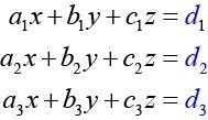
Figure 3
where
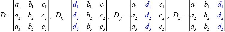
Figure 4
If we are writing the determinant [latex]{D}_{x}[/latex], we replace the [latex]x[/latex] column with the constant column. If we are writing the determinant [latex]{D}_{y}[/latex], we replace the [latex]y[/latex] column with the constant column. If we are writing the determinant [latex]{D}_{z}[/latex], we replace the [latex]z[/latex] column with the constant column. Always check the answer.
Find the solution to the given 3 × 3 system using Cramer’s Rule.
Use Cramer’s Rule.
Then,
The solution is [latex]\left(1,3,-2\right)[/latex].
Use Cramer’s Rule to solve the 3 × 3 matrix.
Solve the system of equations using Cramer’s Rule.
We begin by finding the determinants [latex]D,{D}_{x},\text{and }{D}_{y}[/latex].
We know that a determinant of zero means that either the system has no solution or it has an infinite number of solutions. To see which one, we use the process of elimination. Our goal is to eliminate one of the variables.
We obtain the equation [latex]0=-8[/latex], which is false. Therefore, the system has no solution. Graphing the system reveals two parallel lines.
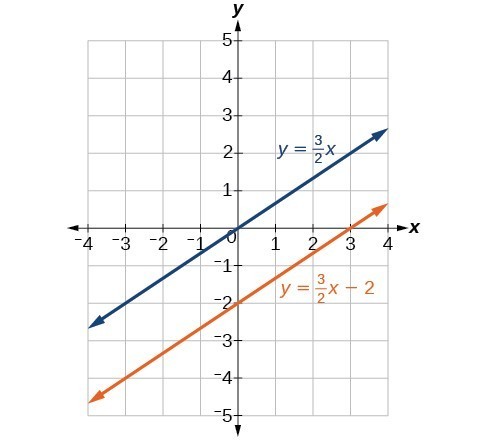
Figure 5
Solve the system with an infinite number of solutions.
Let’s find the determinant first. Set up a matrix augmented by the first two columns.
Then,
As the determinant equals zero, there is either no solution or an infinite number of solutions. We have to perform elimination to find out.
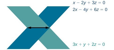
Figure 6
There are many properties of determinants. Listed here are some properties that may be helpful in calculating the determinant of a matrix.
Illustrate each of the properties of determinants.
Property 1 states that if the matrix is in upper triangular form, the determinant is the product of the entries down the main diagonal.
Augment [latex]A[/latex] with the first two columns.
Then
Property 2 states that interchanging rows changes the sign. Given
Property 3 states that if two rows or two columns are identical, the determinant equals zero.
Property 4 states that if a row or column equals zero, the determinant equals zero. Thus,
Property 5 states that the determinant of an inverse matrix [latex]{A}^{-1}[/latex] is the reciprocal of the determinant [latex]A[/latex]. Thus,
Property 6 states that if any row or column of a matrix is multiplied by a constant, the determinant is multiplied by the same factor. Thus,
Find the solution to the given 3 × 3 system.
Using Cramer’s Rule, we have
Notice that the second and third columns are identical. According to Property 3, the determinant will be zero, so there is either no solution or an infinite number of solutions. We have to perform elimination to find out.
Obtaining a statement that is a contradiction means that the system has no solution.
1. [latex]\left(3,-7\right)[/latex]
2. [latex]-10[/latex]
3. [latex]\left(-2,\frac{3}{5},\frac{12}{5}\right)[/latex]
1. A determinant is the sum and products of the entries in the matrix, so you can always evaluate that product—even if it does end up being 0.
3. The inverse does not exist.
5. [latex]-2[/latex]
7. [latex]7[/latex]
9. [latex]-4[/latex]
11. [latex]0[/latex]
13. [latex]-7,990.7[/latex]
15. [latex]3[/latex]
17. [latex]-1[/latex]
19. [latex]224[/latex]
21. [latex]15[/latex]
23. [latex]-17.03[/latex]
25. [latex]\left(1,1\right)[/latex]
27. [latex]\left(\frac{1}{2},\frac{1}{3}\right)[/latex]
29. [latex]\left(2,5\right)[/latex]
31. [latex]\left(-1,-\frac{1}{3}\right)[/latex]
33. [latex]\left(15,12\right)[/latex]
35. [latex]\left(1,3,2\right)[/latex]
37. [latex]\left(-1,0,3\right)[/latex]
39. [latex]\left(\frac{1}{2},1,2\right)[/latex]
41. [latex]\left(2,1,4\right)[/latex]
43. Infinite solutions
45. [latex]24[/latex]
47. [latex]1[/latex]
49. Yes; 18, 38
51. Yes; 33, 36, 37
53. $7,000 in first account, $3,000 in second account.
55. 120 children, 1,080 adult
57. 4 gal yellow, 6 gal blue
59. 13 green tomatoes, 17 red tomatoes
61. Strawberries 18%, oranges 9%, kiwi 10%
63. 100 for movie 1, 230 for movie 2, 312 for movie 3
65. 20–29: 2,100, 30–39: 2,600, 40–49: 825
67. 300 almonds, 400 cranberries, 300 cashews
1. Explain why we can always evaluate the determinant of a square matrix.
2. Examining Cramer’s Rule, explain why there is no unique solution to the system when the determinant of your matrix is 0. For simplicity, use a [latex]2\times 2[/latex] matrix.
3. Explain what it means in terms of an inverse for a matrix to have a 0 determinant.
4. The determinant of [latex]2\times 2[/latex] matrix [latex]A[/latex] is 3. If you switch the rows and multiply the first row by 6 and the second row by 2, explain how to find the determinant and provide the answer.
For the following exercises, find the determinant.
5. [latex]|\begin{array}{cc}1& 2\\ 3& 4\end{array}|[/latex]
6. [latex]|\begin{array}{rr}\hfill -1& \hfill 2\\ \hfill 3& \hfill -4\end{array}|[/latex]
7. [latex]|\begin{array}{rr}\hfill 2& \hfill -5\\ \hfill -1& \hfill 6\end{array}|[/latex]
8. [latex]|\begin{array}{cc}-8& 4\\ -1& 5\end{array}|[/latex]
9. [latex]|\begin{array}{rr}\hfill 1& \hfill 0\\ \hfill 3& \hfill -4\end{array}|[/latex]
10. [latex]|\begin{array}{rr}\hfill 10& \hfill 20\\ \hfill 0& \hfill -10\end{array}|[/latex]
11. [latex]|\begin{array}{cc}10& 0.2\\ 5& 0.1\end{array}|[/latex]
12. [latex]|\begin{array}{rr}\hfill 6& \hfill -3\\ \hfill 8& \hfill 4\end{array}|[/latex]
13. [latex]|\begin{array}{rr}\hfill -2& \hfill -3\\ \hfill 3.1& \hfill 4,000\end{array}|[/latex]
14. [latex]|\begin{array}{rr}\hfill -1.1& \hfill 0.6\\ \hfill 7.2& \hfill -0.5\end{array}|[/latex]
15. [latex]|\begin{array}{rrr}\hfill -1& \hfill 0& \hfill 0\\ \hfill 0& \hfill 1& \hfill 0\\ \hfill 0& \hfill 0& \hfill -3\end{array}|[/latex]
16. [latex]|\begin{array}{rrr}\hfill -1& \hfill 4& \hfill 0\\ \hfill 0& \hfill 2& \hfill 3\\ \hfill 0& \hfill 0& \hfill -3\end{array}|[/latex]
17. [latex]|\begin{array}{ccc}1& 0& 1\\ 0& 1& 0\\ 1& 0& 0\end{array}|[/latex]
18. [latex]|\begin{array}{rrr}\hfill 2& \hfill -3& \hfill 1\\ \hfill 3& \hfill -4& \hfill 1\\ \hfill -5& \hfill 6& \hfill 1\end{array}|[/latex]
19. [latex]|\begin{array}{rrr}\hfill -2& \hfill 1& \hfill 4\\ \hfill -4& \hfill 2& \hfill -8\\ \hfill 2& \hfill -8& \hfill -3\end{array}|[/latex]
20. [latex]|\begin{array}{rrr}\hfill 6& \hfill -1& \hfill 2\\ \hfill -4& \hfill -3& \hfill 5\\ \hfill 1& \hfill 9& \hfill -1\end{array}|[/latex]
21. [latex]|\begin{array}{rrr}\hfill 5& \hfill 1& \hfill -1\\ \hfill 2& \hfill 3& \hfill 1\\ \hfill 3& \hfill -6& \hfill -3\end{array}|[/latex]
22. [latex]|\begin{array}{rrr}\hfill 1.1& \hfill 2& \hfill -1\\ \hfill -4& \hfill 0& \hfill 0\\ \hfill 4.1& \hfill -0.4& \hfill 2.5\end{array}|[/latex]
23. [latex]|\begin{array}{rrr}\hfill 2& \hfill -1.6& \hfill 3.1\\ \hfill 1.1& \hfill 3& \hfill -8\\ \hfill -9.3& \hfill 0& \hfill 2\end{array}|[/latex]
24. [latex]|\begin{array}{ccc}-\frac{1}{2}& \frac{1}{3}& \frac{1}{4}\\ \frac{1}{5}& -\frac{1}{6}& \frac{1}{7}\\ 0& 0& \frac{1}{8}\end{array}|[/latex]
For the following exercises, solve the system of linear equations using Cramer’s Rule.
25. [latex]\begin{array}{l}2x - 3y=-1\\ 4x+5y=9\end{array}[/latex]
26. [latex]\begin{array}{r}5x - 4y=2\\ -4x+7y=6\end{array}[/latex]
27. [latex]\begin{array}{l}\text{ }6x - 3y=2\hfill \\ -8x+9y=-1\hfill \end{array}[/latex]
28. [latex]\begin{array}{l}2x+6y=12\\ 5x - 2y=13\end{array}[/latex]
29. [latex]\begin{array}{l}4x+3y=23\hfill \\ \text{ }2x-y=-1\hfill \end{array}[/latex]
30. [latex]\begin{array}{l}10x - 6y=2\hfill \\ -5x+8y=-1\hfill \end{array}[/latex]
31. [latex]\begin{array}{l}4x - 3y=-3\\ 2x+6y=-4\end{array}[/latex]
32. [latex]\begin{array}{r}4x - 5y=7\\ -3x+9y=0\end{array}[/latex]
33. [latex]\begin{array}{l}4x+10y=180\hfill \\ -3x - 5y=-105\hfill \end{array}[/latex]
34. [latex]\begin{array}{l}\text{ }8x - 2y=-3\hfill \\ -4x+6y=4\hfill \end{array}[/latex]
For the following exercises, solve the system of linear equations using Cramer’s Rule.
35. [latex]\begin{array}{l}\text{ }x+2y - 4z=-1\hfill \\ \text{ }7x+3y+5z=26\hfill \\ -2x - 6y+7z=-6\hfill \end{array}[/latex]
36. [latex]\begin{array}{l}-5x+2y - 4z=-47\hfill \\ \text{ }4x - 3y-z=-94\hfill \\ \text{ }3x - 3y+2z=94\hfill \end{array}[/latex]
37. [latex]\begin{array}{l}\text{ }4x+5y-z=-7\hfill \\ -2x - 9y+2z=8\hfill \\ \text{ }5y+7z=21\hfill \end{array}[/latex]
38. [latex]\begin{array}{r}4x - 3y+4z=10\\ 5x - 2z=-2\\ 3x+2y - 5z=-9\end{array}[/latex]
39. [latex]\begin{array}{l}4x - 2y+3z=6\hfill \\ \text{ }-6x+y=-2\hfill \\ 2x+7y+8z=24\hfill \end{array}[/latex]
40. [latex]\begin{array}{r}\hfill 5x+2y-z=1\\ \hfill -7x - 8y+3z=1.5\\ \hfill 6x - 12y+z=7\end{array}[/latex]
41. [latex]\begin{array}{l}\text{ }13x - 17y+16z=73\hfill \\ -11x+15y+17z=61\hfill \\ \text{ }46x+10y - 30z=-18\hfill \end{array}[/latex]
42. [latex]\begin{array}{l}\begin{array}{l}\hfill \\ -4x - 3y - 8z=-7\hfill \end{array}\hfill \\ \text{ }2x - 9y+5z=0.5\hfill \\ \text{ }5x - 6y - 5z=-2\hfill \end{array}[/latex]
43. [latex]\begin{array}{l}\text{ }4x - 6y+8z=10\hfill \\ -2x+3y - 4z=-5\hfill \\ \text{ }x+y+z=1\hfill \end{array}[/latex]
44. [latex]\begin{array}{r}\hfill 4x - 6y+8z=10\\ \hfill -2x+3y - 4z=-5\\ \hfill 12x+18y - 24z=-30\end{array}[/latex]
For the following exercises, use the determinant function on a graphing utility.
45. [latex]|\begin{array}{rrrr}\hfill 1& \hfill 0& \hfill 8& \hfill 9\\ \hfill 0& \hfill 2& \hfill 1& \hfill 0\\ \hfill 1& \hfill 0& \hfill 3& \hfill 0\\ \hfill 0& \hfill 2& \hfill 4& \hfill 3\end{array}|[/latex]
46. [latex]|\begin{array}{rrrr}\hfill 1& \hfill 0& \hfill 2& \hfill 1\\ \hfill 0& \hfill -9& \hfill 1& \hfill 3\\ \hfill 3& \hfill 0& \hfill -2& \hfill -1\\ \hfill 0& \hfill 1& \hfill 1& \hfill -2\end{array}|[/latex]
47. [latex]|\begin{array}{rrrr}\hfill \frac{1}{2}& \hfill 1& \hfill 7& \hfill 4\\ \hfill 0& \hfill \frac{1}{2}& \hfill 100& \hfill 5\\ \hfill 0& \hfill 0& \hfill 2& \hfill 2,000\\ \hfill 0& \hfill 0& \hfill 0& \hfill 2\end{array}|[/latex]
48. [latex]|\begin{array}{rrrr}\hfill 1& \hfill 0& \hfill 0& \hfill 0\\ \hfill 2& \hfill 3& \hfill 0& \hfill 0\\ \hfill 4& \hfill 5& \hfill 6& \hfill 0\\ \hfill 7& \hfill 8& \hfill 9& \hfill 0\end{array}|[/latex]
For the following exercises, create a system of linear equations to describe the behavior. Then, calculate the determinant. Will there be a unique solution? If so, find the unique solution.
49. Two numbers add up to 56. One number is 20 less than the other.
50. Two numbers add up to 104. If you add two times the first number plus two times the second number, your total is 208
51. Three numbers add up to 106. The first number is 3 less than the second number. The third number is 4 more than the first number.
52. Three numbers add to 216. The sum of the first two numbers is 112. The third number is 8 less than the first two numbers combined.
For the following exercises, create a system of linear equations to describe the behavior. Then, solve the system for all solutions using Cramer’s Rule.
53. You invest $10,000 into two accounts, which receive 8% interest and 5% interest. At the end of a year, you had $10,710 in your combined accounts. How much was invested in each account?
54. You invest $80,000 into two accounts, $22,000 in one account, and $58,000 in the other account. At the end of one year, assuming simple interest, you have earned $2,470 in interest. The second account receives half a percent less than twice the interest on the first account. What are the interest rates for your accounts?
55. A movie theater needs to know how many adult tickets and children tickets were sold out of the 1,200 total tickets. If children’s tickets are $5.95, adult tickets are $11.15, and the total amount of revenue was $12,756, how many children’s tickets and adult tickets were sold?
56. A concert venue sells single tickets for $40 each and couple’s tickets for $65. If the total revenue was $18,090 and the 321 tickets were sold, how many single tickets and how many couple’s tickets were sold?
57. You decide to paint your kitchen green. You create the color of paint by mixing yellow and blue paints. You cannot remember how many gallons of each color went into your mix, but you know there were 10 gal total. Additionally, you kept your receipt, and know the total amount spent was $29.50. If each gallon of yellow costs $2.59, and each gallon of blue costs $3.19, how many gallons of each color go into your green mix?
58. You sold two types of scarves at a farmers’ market and would like to know which one was more popular. The total number of scarves sold was 56, the yellow scarf cost $10, and the purple scarf cost $11. If you had total revenue of $583, how many yellow scarves and how many purple scarves were sold?
59. Your garden produced two types of tomatoes, one green and one red. The red weigh 10 oz, and the green weigh 4 oz. You have 30 tomatoes, and a total weight of 13 lb, 14 oz. How many of each type of tomato do you have?
60. At a market, the three most popular vegetables make up 53% of vegetable sales. Corn has 4% higher sales than broccoli, which has 5% more sales than onions. What percentage does each vegetable have in the market share?
61. At the same market, the three most popular fruits make up 37% of the total fruit sold. Strawberries sell twice as much as oranges, and kiwis sell one more percentage point than oranges. For each fruit, find the percentage of total fruit sold.
62. Three bands performed at a concert venue. The first band charged $15 per ticket, the second band charged $45 per ticket, and the final band charged $22 per ticket. There were 510 tickets sold, for a total of $12,700. If the first band had 40 more audience members than the second band, how many tickets were sold for each band?
63. A movie theatre sold tickets to three movies. The tickets to the first movie were $5, the tickets to the second movie were $11, and the third movie was $12. 100 tickets were sold to the first movie. The total number of tickets sold was 642, for a total revenue of $6,774. How many tickets for each movie were sold?
64. Men aged 20–29, 30–39, and 40–49 made up 78% of the population at a prison last year. This year, the same age groups made up 82.08% of the population. The 20–29 age group increased by 20%, the 30–39 age group increased by 2%, and the 40–49 age group decreased to [latex]\frac{3}{4}[/latex] of their previous population. Originally, the 30–39 age group had 2% more prisoners than the 20–29 age group. Determine the prison population percentage for each age group last year.
65. At a women’s prison down the road, the total number of inmates aged 20–49 totaled 5,525. This year, the 20–29 age group increased by 10%, the 30–39 age group decreased by 20%, and the 40–49 age group doubled. There are now 6,040 prisoners. Originally, there were 500 more in the 30–39 age group than the 20–29 age group. Determine the prison population for each age group last year.
For the following exercises, use this scenario: A health-conscious company decides to make a trail mix out of almonds, dried cranberries, and chocolate-covered cashews. The nutritional information for these items is shown below.
| Fat (g) | Protein (g) | Carbohydrates (g) | |
|---|---|---|---|
| Almonds (10) | 6 | 2 | 3 |
| Cranberries (10) | 0.02 | 0 | 8 |
| Cashews (10) | 7 | 3.5 | 5.5 |
66. For the special “low-carb”trail mix, there are 1,000 pieces of mix. The total number of carbohydrates is 425 g, and the total amount of fat is 570.2 g. If there are 200 more pieces of cashews than cranberries, how many of each item is in the trail mix?
67. For the “hiking” mix, there are 1,000 pieces in the mix, containing 390.8 g of fat, and 165 g of protein. If there is the same amount of almonds as cashews, how many of each item is in the trail mix?
68. For the “energy-booster” mix, there are 1,000 pieces in the mix, containing 145 g of protein and 625 g of carbohydrates. If the number of almonds and cashews summed together is equivalent to the amount of cranberries, how many of each item is in the trail mix?
For the following exercises, determine whether each of the following relations is a function.
1. y = 2x + 8
2. [latex]\left\{\left(2,1\right),\left(3,2\right),\left(-1,1\right),\left(0,-2\right)\right\}\\[/latex]
For the following exercises, evaluate the function [latex]f\left(x\right)=-3{x}^{2}+2x\\[/latex] at the given input.
3. [latex]f\left(-2\right)\\[/latex]
4. [latex]f\left(a\right)\\[/latex]
5. Show that the function [latex]f\left(x\right)=-2{\left(x - 1\right)}^{2}+3\\[/latex] is not one-to-one.
6. Write the domain of the function [latex]f\left(x\right)=\sqrt{3-x}\\[/latex] in interval notation.
7. Given [latex]f\left(x\right)=2{x}^{2}-5x\\[/latex], find [latex]f\left(a+1\right)-f\left(1\right)\\[/latex].
8. Graph the function [latex]\begin{cases}f\left(x\right) & =x+1 & \text{ if }-2 < x < 3 \\ \text{ }& =-x & \text{ if }x\ge 3\end{cases}\\[/latex]
9. Find the average rate of change of the function [latex]f\left(x\right)=3 - 2{x}^{2}+x\\[/latex] by finding [latex]\frac{f\left(b\right)-f\left(a\right)}{b-a}\\[/latex].
For the following exercises, use the functions [latex]f\left(x\right)=3 - 2{x}^{2}+x\text{ and }g\left(x\right)=\sqrt{x}\\[/latex] to find the composite functions.
10. [latex]\left(g\circ f\right)\left(x\right)\\[/latex]
11. [latex]\left(g\circ f\right)\left(1\right)\\[/latex]
12. Express [latex]H\left(x\right)=\sqrt[3]{5{x}^{2}-3x}\\[/latex] as a composition of two functions, f and g, where [latex]\left(f\circ g\right)\left(x\right)=H\left(x\right)\\[/latex].
For the following exercises, graph the functions by translating, stretching, and/or compressing a toolkit function.
13. [latex]f\left(x\right)=\sqrt{x+6}-1\\[/latex]
14. [latex]f\left(x\right)=\frac{1}{x+2}-1\\[/latex]
For the following exercises, determine whether the functions are even, odd, or neither.
15. [latex]f\left(x\right)=-\frac{5}{{x}^{2}}+9{x}^{6}\\[/latex]
16. [latex]f\left(x\right)=-\frac{5}{{x}^{3}}+9{x}^{5}\\[/latex]
17. [latex]f\left(x\right)=\frac{1}{x}\\[/latex]
18. Graph the absolute value function [latex]f\left(x\right)=-2|x - 1|+3\\[/latex].
19. Solve [latex]|2x - 3|=17\\[/latex].
20. Solve [latex]-|\frac{1}{3}x - 3|\ge 17\\[/latex]. Express the solution in interval notation.
For the following exercises, find the inverse of the function.
21. [latex]f\left(x\right)=3x - 5\\[/latex]
22. [latex]f\left(x\right)=\frac{4}{x+7}\\[/latex]
For the following exercises, use the graph of g shown below.

23. On what intervals is the function increasing?
24. On what intervals is the function decreasing?
25. Approximate the local minimum of the function. Express the answer as an ordered pair.
26. Approximate the local maximum of the function. Express the answer as an ordered pair.
For the following exercises, use the graph of the piecewise function shown below.

27. Find [latex]f\left(2\right)\\[/latex].
28. Find [latex]f\left(-2\right)\\[/latex].
29. Write an equation for the piecewise function.
For the following exercises, use the values listed below.
| x | F(x) |
| 0 | 1 |
| 1 | 3 |
| 2 | 5 |
| 3 | 7 |
| 4 | 9 |
| 5 | 11 |
| 6 | 13 |
| 7 | 15 |
| 8 | 17 |
30. Find [latex]F\left(6\right)\\[/latex].
31. Solve the equation [latex]F\left(x\right)=5\\[/latex].
32. Is the graph increasing or decreasing on its domain?
33. Is the function represented by the graph one-to-one?
34. Find [latex]{F}^{-1}\left(15\right)\\[/latex].
35. Given [latex]f\left(x\right)=-2x+11\\[/latex], find [latex]{f}^{-1}\left(x\right)\\[/latex].
1. The relation is a function.
3. −16
5. The graph is a parabola and the graph fails the horizontal line test.
7. [latex]2{a}^{2}-a\\[/latex]
9. [latex]-2\left(a+b\right)+1\\[/latex]
11. [latex]\sqrt{2}\\[/latex]
13.

15. even
17. odd
19. x = –7 and x = 10
21. [latex]{f}^{-1}\left(x\right)=\frac{x+5}{3}\\[/latex]
23. [latex]\left(-\infty ,-1.1\right)\text{ and }\left(1.1,\infty \right)\\[/latex]
25. [latex]\left(1.1,-0.9\right)\\[/latex]
27. [latex]f\left(2\right)=2\\[/latex]
29. [latex]f\left(x\right)=\begin{cases}|x|\text{ if }x\le 2\\ 3\text{ if }x>2\end{cases}\\[/latex]
31. [latex]x=2\\[/latex]
33. yes
35. [latex]{f}^{-1}\left(x\right)=-\frac{x - 11}{2}\\[/latex]
1. Determine whether the following algebraic equation can be written as a linear function. 2x + 3y = 7
2. Determine whether the following function is increasing or decreasing. f(x) = –2x + 5
3. Determine whether the following function is increasing or decreasing. f(x) = 7x + 9
4. Given the following set of information, find a linear equation satisfying the conditions, if possible.
Passes through (5, 1) and (3, –9)
5. Given the following set of information, find a linear equation satisfying the conditions, if possible.
x intercept at (–4, 0) and y-intercept at (0, –6)
6. Find the slope of the line in the graph below.
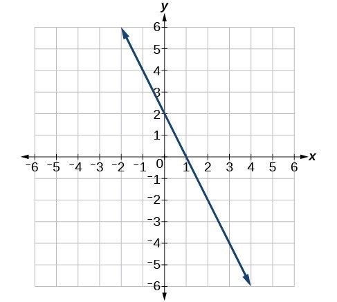
7. Write an equation for line in the graph below.
8. Does the table below represent a linear function? If so, find a linear equation that models the data.
| x | –6 | 0 | 2 | 4 |
| g(x) | 14 | 32 | 38 | 44 |
9. Does the table below represent a linear function? If so, find a linear equation that models the data.
| x | 1 | 3 | 7 | 11 |
| g(x) | 4 | 9 | 19 | 12 |
10. At 6 am, an online company has sold 120 items that day. If the company sells an average of 30 items per hour for the remainder of the day, write an expression to represent the number of items that were sold [latex]n[/latex] after 6 am.
For the following exercises, determine whether the lines given by the equations below are parallel, perpendicular, or neither parallel nor perpendicular:
11. [latex]\begin{cases} y=\frac{3}{4}x - 9\hfill \\ -4x - 3y=8\hfill \end{cases}\\[/latex]
12. [latex]\begin{cases} -2x+y=3\hfill \\ 3x+\frac{3}{2}y=5\hfill \end{cases}\\[/latex]
13. Find the x- and y-intercepts of the equation 2x + 7y = –14.
14. Given below are descriptions of two lines. Find the slopes of Line 1 and Line 2. Is the pair of lines parallel, perpendicular, or neither?
Line 1: Passes through (–2, –6) and (3, 14)
Line 2: Passes through (2, 6) and (4, 14)
15. Write an equation for a line perpendicular to f(x) = 4x + 3 and passing through the point (8, 10).
16. Sketch a line with a y-intercept of (0, 5) and slope [latex]-\frac{5}{2}\\[/latex] .
17. Graph the linear function f(x) = –x + 6 .
18. For the two linear functions, find the point of intersection: [latex]\begin{cases}x=y+2\\ 2x - 3y=-1\end{cases}\\[/latex]
19. A car rental company offers two plans for renting a car.
Plan A: $25 per day and $0.10 per mile
Plan B: $40 per day with free unlimited mileage
How many miles would you need to drive for plan B to save you money?
20. Find the area of a triangle bounded by the y axis, the line f(x) = 12 – 4x, and the line perpendicular to f that passes through the origin.
21. A town’s population increases at a constant rate. In 2010 the population was 65,000. By 2012 the population had increased to 90,000. Assuming this trend continues, predict the population in 2018.
22. The number of people afflicted with the common cold in the winter months dropped steadily by 25 each year since 2002 until 2012. In 2002, 8,040 people were inflicted. Find the linear function that models the number of people afflicted with the common cold C as a function of the year, t. When will less than 6,000 people be afflicted?
For the following exercises, use the graph below, showing the profit, y, in thousands of dollars, of a company in a given year, x, where x represents years since 1980.
23. Find the linear function y, where y depends on x, the number of years since 1980.
24. Find and interpret the y-intercept.
25. In 2004, a school population was 1250. By 2012 the population had dropped to 875. Assume the population is changing linearly.
a. How much did the population drop between the year 2004 and 2012?
b. What is the average population decline per year?
c. Find an equation for the population, P, of the school t years after 2004.
26. Draw a scatter plot for the data provided below. Then determine whether the data appears to be linearly related.
| 0 | 2 | 4 | 6 | 8 | 10 |
| –450 | –200 | 10 | 265 | 500 | 755 |
27. Draw a best-fit line for the plotted data.
For the following exercises, use the table below, which shows the percent of unemployed persons 25 years or older who are college graduates in a particular city, by year.
| Year | Percent Graduates |
| 2000 | 8.5 |
| 2002 | 8.0 |
| 2005 | 7.2 |
| 2007 | 6.7 |
| 2010 | 6.4 |
28. Determine whether the trend appears linear. If so, and assuming the trend continues, find a linear regression model to predict the percent of unemployed in a given year to three decimal places.
29. In what year will the percentage drop below 4%?
30. Based on the set of data given in the table below, calculate the regression line using a calculator or other technology tool, and determine the correlation coefficient. Round to three decimal places of accuracy.
| x | 16 | 18 | 20 | 24 | 26 |
| y | 106 | 110 | 115 | 120 | 125 |
For the following exercises, consider this scenario: The population of a city increased steadily over a ten-year span. The following ordered pairs shows the population (in hundreds) and the year over the ten-year span, (population, year) for specific recorded years:
(4,500, 2000); (4,700, 2001); (5,200, 2003); (5,800, 2006)
31. Use linear regression to determine a function y, where the year depends on the population. Round to three decimal places of accuracy.
32. Predict when the population will hit 20,000.
33. What is the correlation coefficient for this model?
1. Yes.
3. Increasing
5. y = –1.5x – 6
7. y = –2x – 1
9. No.
11. Perpendicular
13. (–7, 0); (0, –2)
15. y = –0.25x + 12
17.

19. 150
21. 165,000
23. y = 875x + 10,675
25. a) 375
b) dropped an average of 46.875, or about 47 people per year
c) y = –46.875t + 1250
27.

29. Early in 2018
31. y = 0.00455x + 1979.5
33. r = 0.999
1. Determine whether the following algebraic equation can be written as a linear function. 2x + 3y = 7
2. Determine whether the following function is increasing or decreasing. f(x) = –2x + 5
3. Determine whether the following function is increasing or decreasing. f(x) = 7x + 9
4. Given the following set of information, find a linear equation satisfying the conditions, if possible.
Passes through (5, 1) and (3, –9)
5. Given the following set of information, find a linear equation satisfying the conditions, if possible.
x intercept at (–4, 0) and y-intercept at (0, –6)
6. Find the slope of the line.
7. Write an equation for line in the graph below.
8. Does the table below represent a linear function? If so, find a linear equation that models the data.
| x | –6 | 0 | 2 | 4 |
| g(x) | 14 | 32 | 38 | 44 |
9. Does the table below represent a linear function? If so, find a linear equation that models the data.
| x | 1 | 3 | 7 | 11 |
| g(x) | 4 | 9 | 19 | 12 |
10. At 6 am, an online company has sold 120 items that day. If the company sells an average of 30 items per hour for the remainder of the day, write an expression to represent the number of items that were sold n after 6 am.
For the following exercises, determine whether the lines given by the equations below are parallel, perpendicular, or neither parallel nor perpendicular:
11. [latex]\begin{cases} y=\frac{3}{4}x - 9\hfill \\ -4x - 3y=8\hfill \end{cases}\\[/latex]
12. [latex]\begin{cases} -2x+y=3\hfill \\ 3x+\frac{3}{2}y=5\hfill \end{cases}\\[/latex]
13. Find the x- and y-intercepts of the equation 2x + 7y = –14.
14. Given below are descriptions of two lines. Find the slopes of Line 1 and Line 2. Is the pair of lines parallel, perpendicular, or neither?
Line 1: Passes through (–2, –6) and (3, 14)
Line 2: Passes through (2, 6) and (4, 14)
15. Write an equation for a line perpendicular to f(x) = 4x + 3 and passing through the point (8, 10).
16. Sketch a line with a y-intercept of (0, 5) and slope [latex]-\frac{5}{2}\\[/latex] .
17. Graph the linear function f(x) = –x + 6.
18. For the two linear functions, find the point of intersection: [latex]\begin{cases}x=y+2\\ 2x - 3y=-1\end{cases}\\[/latex]
19. A car rental company offers two plans for renting a car.
Plan A: $25 per day and $0.10 per mile
Plan B: $40 per day with free unlimited mileage
How many miles would you need to drive for plan B to save you money?
20. Find the area of a triangle bounded by the y axis, the line f(x) = 12 – 4x, and the line perpendicular to f that passes through the origin.
21. A town’s population increases at a constant rate. In 2010 the population was 65,000. By 2012 the population had increased to 90,000. Assuming this trend continues, predict the population in 2018.
22. The number of people afflicted with the common cold in the winter months dropped steadily by 25 each year since 2002 until 2012. In 2002, 8,040 people were inflicted. Find the linear function that models the number of people afflicted with the common cold C as a function of the year, t. When will less than 6,000 people be afflicted?
For the following exercises, use the graph below, showing the profit, y in thousands of dollars, of a company in a given year, x, where x represents years since 1980.
23. Find the linear function y, where y depends on x, the number of years since 1980.
24. Find and interpret the y-intercept.
25. In 2004, a school population was 1250. By 2012 the population had dropped to 875. Assume the population is changing linearly.
a. How much did the population drop between the year 2004 and 2012?
b. What is the average population decline per year?
c. Find an equation for the population, P, of the school t years after 2004.
26. Draw a scatter plot for the data provided in the table below. Then determine whether the data appears to be linearly related.
| 0 | 2 | 4 | 6 | 8 | 10 |
| –450 | –200 | 10 | 265 | 500 | 755 |
27. Draw a best-fit line for the plotted data.
For the following exercises, use the table below, which shows the percent of unemployed persons 25 years or older who are college graduates in a particular city, by year.
| Year | Percent Graduates |
| 2000 | 8.5 |
| 2002 | 8.0 |
| 2005 | 7.2 |
| 2007 | 6.7 |
| 2010 | 6.4 |
28. Determine whether the trend appears linear. If so, and assuming the trend continues, find a linear regression model to predict the percent of unemployed in a given year to three decimal places.
29. In what year will the percentage drop below 4%?
30. Based on the set of data given below, calculate the regression line using a calculator or other technology tool, and determine the correlation coefficient. Round to three decimal places of accuracy.
| x | 16 | 18 | 20 | 24 | 26 |
| y | 106 | 110 | 115 | 120 | 125 |
For the following exercises, consider this scenario: The population of a city increased steadily over a ten-year span. The following ordered pairs shows the population (in hundreds) and the year over the ten-year span, (population, year) for specific recorded years:
(4,500, 2000); (4,700, 2001); (5,200, 2003); (5,800, 2006)
31. Use linear regression to determine a function y, where the year depends on the population. Round to three decimal places of accuracy.
32. Predict when the population will hit 20,000.
33. What is the correlation coefficient for this model?
1. Yes.
3. Increasing
5. y = –1.5x – 6
7. y = –2x – 1
9. No.
11. Perpendicular
13. (–7, 0); (0, –2)
15. y = –0.25x + 12
17.
19. 150
21. 165,000
23. y = 875x + 10,675
25. a) 375
b) dropped an average of 46.875, or about 47 people per year
c) y = –46.875t + 1250
27.
29. Early in 2018
31. y = 0.00455x + 1979.5
33. r = 0.999
1. The population of a pod of bottlenose dolphins is modeled by the function [latex]A\left(t\right)=8{\left(1.17\right)}^{t}\\[/latex], where t is given in years. To the nearest whole number, what will the pod population be after 3 years?
2. Find an exponential equation that passes through the points (0, 4) and (2, 9).
3. Drew wants to save $2,500 to go to the next World Cup. To the nearest dollar, how much will he need to invest in an account now with 6.25% APR, compounding daily, in order to reach his goal in 4 years?
4. An investment account was opened with an initial deposit of $9,600 and earns 7.4% interest, compounded continuously. How much will the account be worth after 15 years?
5. Graph the function [latex]f\left(x\right)=5{\left(0.5\right)}^{-x}\\[/latex] and its reflection across the y-axis on the same axes, and give the y-intercept.
6. The graph shows transformations of the graph of [latex]f\left(x\right)={\left(\frac{1}{2}\right)}^{x}\\[/latex]. What is the equation for the transformation?
7. Rewrite [latex]{\mathrm{log}}_{8.5}\left(614.125\right)=a\\[/latex] as an equivalent exponential equation.
8. Rewrite [latex]{e}^{\frac{1}{2}}=m\\[/latex] as an equivalent logarithmic equation.
9. Solve for x by converting the logarithmic equation [latex]log_{\frac{1}{7}}\left(x\right)=2\\[/latex] to exponential form.
10. Evaluate [latex]\mathrm{log}\left(\text{10,000,000}\right)\\[/latex] without using a calculator.
11. Evaluate [latex]\mathrm{ln}\left(0.716\right)\\[/latex] using a calculator. Round to the nearest thousandth.
12. Graph the function [latex]g\left(x\right)=\mathrm{log}\left(12 - 6x\right)+3\\[/latex].
13. State the domain, vertical asymptote, and end behavior of the function [latex]f\left(x\right)={\mathrm{log}}_{5}\left(39 - 13x\right)+7\\[/latex].
14. Rewrite [latex]\mathrm{log}\left(17a\cdot 2b\right)\\[/latex] as a sum.
15. Rewrite [latex]{\mathrm{log}}_{t}\left(96\right)-{\mathrm{log}}_{t}\left(8\right)\\[/latex] in compact form.
16. Rewrite [latex]{\mathrm{log}}_{8}\left({a}^{\frac{1}{b}}\right)\\[/latex] as a product.
17. Use properties of logarithm to expand [latex]\mathrm{ln}\left({y}^{3}{z}^{2}\cdot \sqrt[3]{x - 4}\right)\\[/latex].
18. Condense the expression [latex]4\mathrm{ln}\left(c\right)+\mathrm{ln}\left(d\right)+\frac{\mathrm{ln}\left(a\right)}{3}+\frac{\mathrm{ln}\left(b+3\right)}{3}\\[/latex] to a single logarithm.
19. Rewrite [latex]{16}^{3x - 5}=1000\\[/latex] as a logarithm. Then apply the change of base formula to solve for [latex]x[/latex] using the natural log. Round to the nearest thousandth.
20. Solve [latex]{\left(\frac{1}{81}\right)}^{x}\cdot \frac{1}{243}={\left(\frac{1}{9}\right)}^{-3x - 1}\\[/latex] by rewriting each side with a common base.
21. Use logarithms to find the exact solution for [latex]-9{e}^{10a - 8}-5=-41\\[/latex] . If there is no solution, write no solution.
22. Find the exact solution for [latex]10{e}^{4x+2}+5=56\\[/latex]. If there is no solution, write no solution.
23. Find the exact solution for [latex]-5{e}^{-4x - 1}-4=64\\[/latex]. If there is no solution, write no solution.
24. Find the exact solution for [latex]{2}^{x - 3}={6}^{2x - 1}\\[/latex]. If there is no solution, write no solution.
25. Find the exact solution for [latex]{e}^{2x}-{e}^{x}-72=0\\[/latex]. If there is no solution, write no solution.
26. Use the definition of a logarithm to find the exact solution for [latex]4\mathrm{log}\left(2n\right)-7=-11\\[/latex]
27. Use the one-to-one property of logarithms to find an exact solution for [latex]\mathrm{log}\left(4{x}^{2}-10\right)+\mathrm{log}\left(3\right)=\mathrm{log}\left(51\right)\\[/latex] If there is no solution, write no solution.
28. The formula for measuring sound intensity in decibels D is defined by the equation [latex]D=10\mathrm{log}\left(\frac{I}{{I}_{0}}\right)\\[/latex], where I is the intensity of the sound in watts per square meter and [latex]{I}_{0}={10}^{-12}\\[/latex] is the lowest level of sound that the average person can hear. How many decibels are emitted from a rock concert with a sound intensity of [latex]4.7\cdot {10}^{-1}\\[/latex] watts per square meter?
29. A radiation safety officer is working with 112 grams of a radioactive substance. After 17 days, the sample has decayed to 80 grams. Rounding to five significant digits, write an exponential equation representing this situation. To the nearest day, what is the half-life of this substance?
30. Write the formula found in the previous exercise as an equivalent equation with base [latex]e[/latex]. Express the exponent to five significant digits.
31. A bottle of soda with a temperature of 71º Fahrenheit was taken off a shelf and placed in a refrigerator with an internal temperature of 35º F. After ten minutes, the internal temperature of the soda was 63º F. Use Newton’s Law of Cooling to write a formula that models this situation. To the nearest degree, what will the temperature of the soda be after one hour?
32. The population of a wildlife habitat is modeled by the equation [latex]P\left(t\right)=\frac{360}{1+6.2{e}^{-0.35t}}\\[/latex], where t is given in years. How many animals were originally transported to the habitat? How many years will it take before the habitat reaches half its capacity?
33. Enter the data from the table below into a graphing calculator and graph the resulting scatter plot. Determine whether the data from the table would likely represent a function that is linear, exponential, or logarithmic.
| x | f(x) |
| 1 | 3 |
| 2 | 8.55 |
| 3 | 11.79 |
| 4 | 14.09 |
| 5 | 15.88 |
| 6 | 17.33 |
| 7 | 18.57 |
| 8 | 19.64 |
| 9 | 20.58 |
| 10 | 21.42 |
34. The population of a lake of fish is modeled by the logistic equation [latex]P\left(t\right)=\frac{16,120}{1+25{e}^{-0.75t}}\\[/latex], where t is time in years. To the nearest hundredth, how many years will it take the lake to reach 80% of its carrying capacity?
For the following exercises, use a graphing utility to create a scatter diagram of the data given in the table. Observe the shape of the scatter diagram to determine whether the data is best described by an exponential, logarithmic, or logistic model. Then use the appropriate regression feature to find an equation that models the data. When necessary, round values to five decimal places.
35.
| x | f(x) |
| 1 | 20 |
| 2 | 21.6 |
| 3 | 29.2 |
| 4 | 36.4 |
| 5 | 46.6 |
| 6 | 55.7 |
| 7 | 72.6 |
| 8 | 87.1 |
| 9 | 107.2 |
| 10 | 138.1 |
36.
| x | f(x) |
| 3 | 13.98 |
| 4 | 17.84 |
| 5 | 20.01 |
| 6 | 22.7 |
| 7 | 24.1 |
| 8 | 26.15 |
| 9 | 27.37 |
| 10 | 28.38 |
| 11 | 29.97 |
| 12 | 31.07 |
| 13 | 31.43 |
37.
| x | f(x) |
| 0 | 2.2 |
| 0.5 | 2.9 |
| 1 | 3.9 |
| 1.5 | 4.8 |
| 2 | 6.4 |
| 3 | 9.3 |
| 4 | 12.3 |
| 5 | 15 |
| 6 | 16.2 |
| 7 | 17.3 |
| 8 | 17.9 |
1. About 13 dolphins.
3. $1,947
5. y-intercept: (0, 5)

7. [latex]{8.5}^{a}=614.125\\[/latex]
9. [latex]x={\left(\frac{1}{7}\right)}^{2}=\frac{1}{49}\\[/latex]
11. [latex]\mathrm{ln}\left(0.716\right)\approx -0.334\\[/latex]
13. Domain: x < 3; Vertical asymptote: x = 3; End behavior: [latex]x\to {3}^{-},f\left(x\right)\to -\infty \\[/latex] and [latex]x\to -\infty ,f\left(x\right)\to \infty \\[/latex]
15. [latex]{\mathrm{log}}_{t}\left(12\right)\\[/latex]
17. [latex]3\mathrm{ln}\left(y\right)+2\mathrm{ln}\left(z\right)+\frac{\mathrm{ln}\left(x - 4\right)}{3}\\[/latex]
19. [latex]x=\frac{\frac{\mathrm{ln}\left(1000\right)}{\mathrm{ln}\left(16\right)}+5}{3}\approx 2.497\\[/latex]
21. [latex]a=\frac{\mathrm{ln}\left(4\right)+8}{10}\\[/latex]
23. no solution
25. [latex]x=\mathrm{ln}\left(9\right)\\[/latex]
27. [latex]x=\pm \frac{3\sqrt{3}}{2}\\[/latex]
29. [latex]f\left(t\right)=112{e}^{-.019792t}\\[/latex]; half-life: about 35 days
31. [latex]T\left(t\right)=36{e}^{-0.025131t}+35;T\left(60\right)\approx {43}^{\text{o}}\text{F}\\[/latex]
33. logarithmic

35. exponential; [latex]y=15.10062{\left(1.24621\right)}^{x}\\[/latex]

37. logistic; [latex]y=\frac{18.41659}{1+7.54644{e}^{-0.68375x}}\\[/latex]

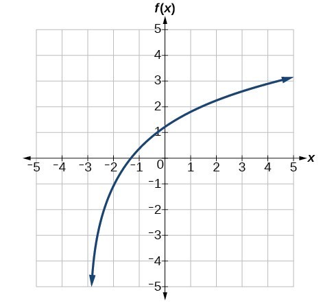
Analysis of the Solution
Although we have seen that we can find the complex conjugate of an imaginary number, in practice we generally find the complex conjugates of only complex numbers with both a real and an imaginary component. To obtain a real number from an imaginary number, we can simply multiply by i.