Not Your Physicists' Entropy
Information Theory Applications to the Nuclear Fuel Cycle
What is the Nuclear Fuel Cycle?
Well, we can ask wikipedia...
How do we model the fuel cycle?
- Most simulations are formulated on premade base-case scenarios:

- These base cases are very well studied.
- However, what is not well known is how these sample scenarios are affected by perturbations to their initial physical parameters.
Problem Space

Figure 1: Physics Modeled versus Execution Time
Modeling Approaches

| Component | Recipes | Essential | Transport |
|---|---|---|---|
| Front End: | Recipes | Physics Models | Physics Models |
| Reactor: | Recipes | Rapid Burnup Code (Bright) | Neutron Transport |
| Repository: | Curve Fits | Rapid Code (Cyder) | Neutron Transport |
Motivation
- Investigating the region of interest may provide a transformative amount of fuel cycle data.
However, this requires an entirely new spectrum of tools.

Figure 2: Fuel Cycle Stack
Definition
Essential physics models remain physically valid under perturbations in the locality of the region on which they are defined and do not compute extraneous parameters.
This is a form of model reduction.
What do Essential Physics Models Buy Us?
They allow us to run physically meaningful (if not economically, etc.) fuel cycle simulations.
And not just a few of them, but many.
And when we have many similar things we use (fancy?!) statistics to analyze the ensemble.
Essential Physics Fuel Cycle Facility Models
One-Group Reactor Model (R1G)

Figure 3: Reactor Model [1]
R1G Notation
| Name | Symbol | Units |
|---|---|---|
| Fluence | $F = \int_0^t \phi dt^\prime = \phi \int_0^t dt^\prime = \phi \times t \cdot \frac{24 \cdot 3600 \cdot 10^3}{10^{24}}$ | [n/kb] |
| Nuclide Subscript | $i$ (or $j$) | [1/kg$_i$] |
| Region Superscript | $Q$ | [unitless] |
| Mass Weights | $m_i^Q = \frac{N_i^Q}{N_{\mbox{IHM}}} = \frac{n_i^Q A_i}{A_{\mbox{IHM}}} \cdot \frac{\rho^Q\cdot\mbox{MW}^F}{\rho^F\cdot\mbox{MW}^Q} \frac{V^Q}{V^F}$ | [kg$_i^Q$/kgIHM] |
| Burnup | $\mbox{BU}(F) = \sum_i m_i^F \cdot \mbox{BU}_i(F)$ | [MWd/kgIHM] |
| Prod & Des Rates | $p_i(F), d_i(F)$ | [n/s/flux/kg$_i$] |
| Transmutation Matrix | $T_{ij}(F)$ | [kg$_j$/kg$_i$] |
| Multiplication Factor | $k(F) = \frac{P(F)}{D(F)}$ | [unitless] |
R1G Library
Starting with ORIGEN generated fluence-dependent, nuclide specific data, we know:
 |  | |
| (a) neutron production & destruction rates, | (b) burnups, | (c) transmutation matrices. |
Figure 4: Example Reactor Data Library for FR $^{239}$Pu
R1G Library Collapse
- Collapsing a general library down is the central calculation of the one-group reactor model.
- Using a two-region fuel pin cell model, denote the mass weight of each initial isotope $i$ in the fuel as $m^F_i$ and the in the coolant as $m^C_i$.
- Then, a mass-weighted linear combination of all of the library parameters computes the full-core values.
- For example,


R1G
 |  |
| (a) burnup | (b) multiplication factor |
Figure 5: Linearly Combined Fast Reactor Data Library
R1G
Figure 6: Fast Reactor Discharge Composition
- The transmutation matrices may be similarly weighted by initial composition.
- From the criticality calculation above we also know the discharge fluence, Fd [n/kb], which will then yield the used fuel vector.
R1G Benchmark
Table 2: LWR Benchmark to OECD Burnup Credit [2]
| Nuclide | OECD [2] [w/o] | $\sigma$ of OECD [%] | Results [w/o] | % Difference |
|---|---|---|---|---|
| $^{234}$U | 0.0178 | 9.0 | 0.0184 | +3.6 |
| $^{235}$U | 0.8001 | 8.1 | 0.7079 | -11.5 |
| $^{236}$U | 0.4840 | 2.6 | 0.4781 | -1.2 |
| $^{238}$U | 93.3333 | 0.2 | 93.6109 | +0.3 |
| $^{237}$Np | 0.0614 | 9.4 | 0.0584 | -5.0 |
| $^{238}$Pu | 0.0226 | 13.9 | 0.0185 | -18.1 |
| $^{239}$Pu | 0.5991 | 7.1 | 0.5104 | +14.8 |
| $^{240}$Pu | 0.2389 | 5.3 | 0.2591 | +8.5 |
| $^{241}$Pu | 0.1636 | 6.9 | 0.1445 | -11.7 |
| $^{242}$Pu | 0.0602 | 8.4 | 0.0563 | -6.5 |
| $^{241}$Am | 0.0047 | 5.3 | 0.0032 | -30.8 |
| $^{243}$Am | 0.0148 | 10.4 | 0.0116 | -21.3 |
R1G Benchmark Notes
- This benchmark compares an OECD study for a 40 MWd/kgIHM burn with no cooling.
- This result shows the R1G matches the burnup credit to within two standard deviations for most actinides.
- $^{241}$Am is the only nuclide showing a relatively higher departure.
- This species is formed through $^{241}$Pu decay.
- $^{241}$Am would thus match better if a constant flux or if zero reloading times were not assumed.
Multigroup Reactor Model (RMG)
- In the R1G, fluxes are assumed to be static over the course of the burn.
- This restricts the types of reactors and fuel cycles which may be modeled. (MOX, IMF, Traveling Wave, etc. are unavailable to the R1G.)
- Also in the R1G, changing reactor state variables in a way that would affect the flux spectrum required additional libraries, or inter-library interpolations.
RMG
- To solve these issues, moving to a multi-energy group reactor model will enable automatic spectral shifts in the core as needed.
- Rather than parameterizing burnup, transmutation, and neutron production & destruction rates as functions of nuclide and fluence, the RMG parameterizes cross sections over a number of different states.
- The R1G parameters are explicitly solved for by the RMG model.
RMG
- Group constants are denoted by $\sigma_{r_x,i\tau g}$ or $\sigma_{r_x,ipg}$ [b].
- Group-to-group scattering by $\sigma_{s,i\tau g\to h}$ or $\sigma_{s,ipg\to h}$.
Table 8: Cross Section Indices
| Index | Symbol |
|---|---|
| Nuclide | $i$ |
| Time | $\tau$ |
| Perturbation | $p$ |
| Incident Energy Group | $g$ |
| Exiting Energy Group | $h$ |
| Reaction Channel [5] | $r_x$ |
Reactor State Variables
Table 9: Parameters $a_p$ which Define a Perturbation
| Parameter | Symbol | Units |
|---|---|---|
| Fuel Density | $\rho_{\mbox{fuel}}$ | g/cm$^{3}$ |
| Cladding Density | $\rho_{\mbox{clad}}$ | g/cm$^{3}$ |
| Coolant Density | $\rho_{\mbox{cool}}$ | g/cm$^{3}$ |
| Fuel Cell Radius | $r_{\mbox{fuel}}$ | cm |
| Void Cell Radius | $r_{\mbox{void}}$ | cm |
| Cladding Cell Radius | $r_{\mbox{clad}}$ | cm |
| Unit Cell Pitch | $\ell$ | cm |
| Number of Burn Regions | $b_r$ | |
| Fuel Specific Power | $p_s$ | MW/kgIHM |
| Initial Nuclide Mass Fraction | $T_{i0}$ | kg$_i$/kgIHM |
| Burn Times | $s$ | days |
Multicomponent Enrichment Model
Table 10: Outer Product Perturbations
| $\rho_{\mbox{fuel}}$ | $\rho_{\mbox{clad}}$ | $\rho_{\mbox{cool}}$ | $r_{\mbox{fuel}}$ | $r_{\mbox{void}}$ | $r_{\mbox{clad}}$ | $\ell$ | $b_r$ | $p_s$ | $T_{\mbox{$^{235}$U0}}$ | $s$ |
|---|---|---|---|---|---|---|---|---|---|---|
| 10.165 | 5.87 | 0.73 | 0.41 | 0.4185 | 0.475 | 1.3127 | 10 | 0.04 | 0.03 | 0 |
| 10.165 | 5.87 | 0.73 | 0.41 | 0.4185 | 0.475 | 1.3127 | 10 | 0.04 | 0.03 | 100 |
| 10.165 | 5.87 | 0.73 | 0.41 | 0.4185 | 0.475 | 1.3127 | 10 | 0.04 | 0.03 | 200 |
| 10.165 | 5.87 | 0.73 | 0.41 | 0.4185 | 0.475 | 1.3127 | 10 | 0.04 | 0.03 | 300 |
| 10.165 | 5.87 | 0.73 | 0.41 | 0.4185 | 0.475 | 1.3127 | 10 | 0.04 | 0.03 | 400 |
| 10.165 | 5.87 | 0.73 | 0.41 | 0.4185 | 0.475 | 1.3127 | 10 | 0.04 | 0.05 | 0 |
| 10.165 | 5.87 | 0.73 | 0.41 | 0.4185 | 0.475 | 1.3127 | 10 | 0.04 | 0.05 | 100 |
| 10.165 | 5.87 | 0.73 | 0.41 | 0.4185 | 0.475 | 1.3127 | 10 | 0.04 | 0.05 | 200 |
| 10.165 | 5.87 | 0.73 | 0.41 | 0.4185 | 0.475 | 1.3127 | 10 | 0.04 | 0.05 | 200 |
| 10.165 | 5.87 | 0.73 | 0.41 | 0.4185 | 0.475 | 1.3127 | 10 | 0.04 | 0.05 | 300 |
| 10.165 | 5.87 | 0.73 | 0.41 | 0.4185 | 0.475 | 1.3127 | 10 | 0.04 | 0.05 | 400 |
| $\vdots$ | $\vdots$ | $\vdots$ | $\vdots$ | $\vdots$ | $\vdots$ | $\vdots$ | $\vdots$ | $\vdots$ | $\vdots$ | $\vdots$ |
Cross Section Generation
- Cross section generation takes a multi-tier approach.
- For very important nuclides, $\sigma_{pg}$ were found via the Monte Carlo neutron transport code Serpent [6] (slightly modified).
- For important species for which high-fidelity continuous cross section data is not available, physical models and/or a flux weighted collapse of 64-group CINDER data is used.
- For species unimportant to the FC material balance, a simple interpolation between thermal and fast cross sections from KAERI is used to generate group constants.
RMG Methodology
- Once the cross-section library has been assembled, the RMG proceeds in three main calculation routines per time step.
- First, there is as a nearest-neighbor calculation from the given reactor state to the perturbations states in the library.
- A multigroup spectrum-criticality calculation.
- A burnup-transmutation calculation.
Multigroup Reactor Model Flow Diagram

RMG Metric Space
- With $p$ as the perturbation index ($1 \le p \le n_p$), $a_p$ is a parameter value in the library and $a_r$ the value on the reactor at run time.
- The distance from any perturbation to the current reactor is given by $d_p$:
- The sequence $p^\star$ determines the nearest neighbors:
Cross Section Interpolation
- Using the shorthand $a_p^\star$ as a substitute for $a_{p^\star}$,
- Then $x_f$ is a unitless multidimensional linear interpolation factor,
- Group constants for each time step are computed:
Criticality Calculation
- The shape of the spectrum is given by an iterative solution to a matrix method.
- ...with a rescaling to obtain the magnitude,
- and a side calculation to obtain the multiplication factor.
Transmutation Calculation
- ORIGEN 2.2 [7] is used as the transmutation kernel for the RMG.
- Custom ORIGEN cross section libraries are built for each time step. The group constants for the current reactor state are simply collapsed.
RMG Benchmark
- The RMG was benchmarked against a Serpent run where both transport and essential physics methods were fed the OECD's LWR Burnup Credit reactor [2].
- The benchmark examines the first year of the burn with an initial $^{235}$U enrichment of 4.5 [w/o].
RMG Benchmark
Table 11: Nearest Neighbors over Burn
| days | $p^\star=1$ | 2 | 3 | 4 | 5 | 6 | 7 | 8 | 9 | 10 | 11 | 12 | 13 | 14 | 15 | 16 | $\cdots$ |
|---|---|---|---|---|---|---|---|---|---|---|---|---|---|---|---|---|---|
| 0 | 16 | 6 | 17 | 7 | 18 | 8 | 11 | 1 | 9 | 19 | 12 | 2 | 13 | 3 | 10 | 20 | $\cdots$ |
| 40.6 | 16 | 6 | 17 | 7 | 18 | 8 | 19 | 9 | 11 | 1 | 12 | 2 | 13 | 3 | 10 | 20 | $\cdots$ |
| 81.1 | 17 | 7 | 16 | 6 | 18 | 8 | 19 | 9 | 2 | 12 | 11 | 1 | 13 | 3 | 10 | 20 | $\cdots$ |
| 122 | 7 | 17 | 18 | 8 | 6 | 16 | 19 | 9 | 20 | 10 | 2 | 12 | 3 | 13 | 11 | 1 | $\cdots$ |
| 162 | 8 | 18 | 7 | 17 | 19 | 9 | 6 | 16 | 20 | 10 | 3 | 13 | 2 | 12 | 4 | 14 | $\cdots$ |
| 203 | 18 | 8 | 19 | 9 | 17 | 7 | 10 | 20 | 6 | 16 | 3 | 13 | 4 | 14 | 12 | 2 | $\cdots$ |
| 243 | 18 | 8 | 19 | 9 | 17 | 7 | 10 | 20 | 6 | 16 | 3 | 13 | 4 | 14 | 12 | 2 | $\cdots$ |
| 284 | 19 | 9 | 18 | 8 | 10 | 20 | 7 | 17 | 4 | 14 | 6 | 16 | 3 | 13 | 5 | 15 | $\cdots$ |
| 324 | 19 | 9 | 10 | 20 | 8 | 18 | 7 | 17 | 4 | 14 | 5 | 15 | 3 | 13 | 6 | 16 | $\cdots$ |
| 365 | 10 | 20 | 19 | 9 | 18 | 8 | 7 | 17 | 5 | 15 | 4 | 14 | 3 | 13 | 6 | 16 | $\cdots$ |
RMG Benchmark

Figure 20: Multiplication Factor Benchmark
RMG Benchmark
 |  |
| (a) BOL | (b) EOL |
Figure 21: Neutron Flux Spectrum Benchmarks
RMG Benchmark
 |  |  |
| (a) $^{235}$U | (b) $^{246}$Cm | (c) $^{137}$Cs |
Figure 22: Selected Mass Fractions
RMG Benchmark
 |  |  |
| (a) $^{235}$U | (b) $^{239}$Pu | (c) $^{99}$Tc |
Figure 23: Selected One-Group Cross-Sections
Multicomponent Enrichment Model
Here are the matched abundance ratio cascade equations:
What if we solved these equations symbolically, rather than numerically..
Multicomponent Enrichment
...and use code generation to produce a blazing solver.


Multicomponent Enrichment
We get really big speedups (20-300x)!
 |  |
| (a) per iteration | (b) over minimzation |
Figure 23: Execution Timing Comparison
See http://pynesim.org/usersguide/enrichment.html for more details.
Fuel Cycle Sensitivity Study
Sensitivty Study Overview
- Here, the system-wide impact of physical parameter perturbations is quantified.
- This is done by looking for linear, 1D sensitivity coefficients for each parameter to the repository capacity response, measured in [PWh].
- Denote these sensitivity coefficients as $S_x$ for a small change in an input parameter $x$.
- Sensitivity coefficients are presented for 10% changes in $x$ from assumed base-case values.
Sensitivity Methodology Algorithm
1. For each input parameter $x$, change its base-case value $x_0$ by $\pm10\%$.
2. If $x$ is a separation efficiency (SE), instead perturb by $\pm$ "one nine" worth of separations.
3. Meanwhile, maintain all other parameters ($y, z, \ldots$) at their base-case values.
4. Calculate the new repository capacity response, $R$, by the perturbed cycle and record the sensitivity as the percent change from the base-case response, $R_0$.
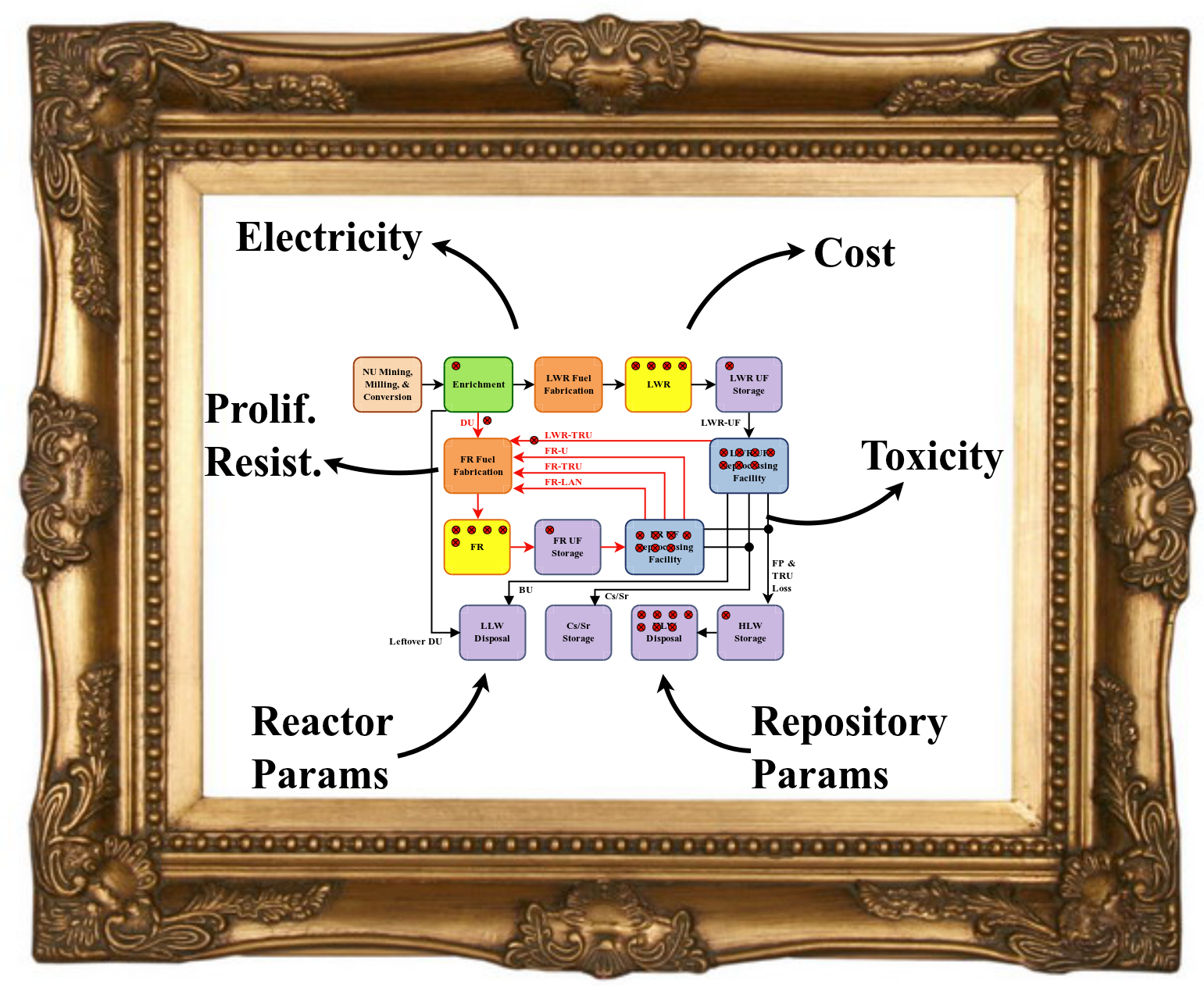
Fuel Cycle
The essential physics models from before were used to study a Fast Reactor, Light Water Reactor symbiotic scenario analogous to Scheme 3a of a 2006 OECD report [3].

Fuel Cycle
With perturbable components, over 30 independent physical parameters may be adjusted in the fuel cycle. Sensitivity results are computed from equilibrium values derived from a full treatment of the preceding, transient cycles.

Base Case Parameter Definition
| Input Parameter $x$ | Value | Units |
|---|---|---|
| LWR Burnup | 50.0 | MWd/kgIHM |
| LWR Fuel to Moderator Ratio | 0.301 | |
| LWR UF Storage Time | 60 | years |
| SE of U from LWR UF | 0.999 | |
| SE of NP from LWR UF | 0.999 | |
| SE of PU from LWR UF | 0.999 | |
| SE of AM from LWR UF | 0.999 | |
| SE of CM from LWR UF | 0.999 | |
| SE of CS from LWR UF | 0.999 | |
| SE of SR from LWR UF | 0.999 | |
| FR Burnup | 140.0 | MWd/kgIHM |
| FR TRU Conversion Ratio | 0.50 | |
| Max Fraction of Lanthanide in FR Fuel | 0.0005 | Atoms/TRU Atom |
| FR UF Storage Time | 3 | years |
| Storage Before Disposal | 50 | years |
Base Case Parameter Definition
| Input Parameter $x$ | Value | Units |
|---|---|---|
| SE of U from FR UF | 0.999 | |
| SE of NP from FR UF | 0.999 | |
| SE of PU from FR UF | 0.999 | |
| SE of AM from FR UF | 0.999 | |
| SE of CM from FR UF | 0.999 | |
| SE of CS from FR UF | 0.999 | |
| SE of SR from FR UF | 0.999 | |
| Density of Host Rock | 2580 | kg/m$^{3}$ |
| Specific Heat of Host Rock | 840 | J/kg-K |
| Thermal Conductivity of Host Rock | 1.626 | W/m-K |
| Heat Loss Factor During Ventilation | 0.7 | |
| Drift diameter | 5.5 | m |
| Ventilation System On Time | 50 | years |
| Ambient Environment Temperature | 20 | C |
| Distance Between Drifts | 81 | m |
Fuel Cycle Base Case Benchmark
| Scheme 3a | NEA [3] | Model$^{1}$ | % Diff | Model$^{2}$ | % Diff |
|---|---|---|---|---|---|
| Electricity Share: LWR | 0.632 | 0.619459 | -2.0244 | 0.634907 | +0.4579 |
| Electricity Share: FR | 0.368 | 0.380541 | +3.2955 | 0.365093 | -0.7962 |
| FR UF: U | 0.698 | 0.713806 | +2.2143 | 0.715224 | +2.4082 |
| FR UF: NP | 0.0065 | 0.00661961 | +1.8070 | 0.00685174 | +5.1335 |
| FR UF: PU | 0.266 | 0.248059 | -7.2327 | 0.248319 | -7.1204 |
| FR UF: AM | 0.02 | 0.0226796 | 11.8152 | 0.0217317 | +7.9687 |
| FR UF: CM | 0.0098 | 0.00883517 | -10.920 | 0.00787319 | -24.4730 |
| HLW: U | 0.013324 | 0.0132681 | -0.4213 | 0.0134448 | +0.8984 |
| HLW: NP | 2.26542E-05 | 2.4079E-05 | +5.9173 | 2.41083E-05 | +6.0316 |
| HLW: PU | 0.000704797 | 0.000658893 | -6.9668 | 0.000632361 | -11.4548 |
| HLW: AM | 5.03426E-05 | 5.63068E-05 | 10.5923 | 5.12344E-05 | +1.7405 |
| HLW: CM | 2.18151E-05 | 1.99031E-05 | -9.6068 | 1.67094E-05 | -30.5563 |
| HLW: FP | 0.985876 | 0.985973 | +0.0098 | 0.985831 | -0.0046 |
- Model with initial LWR $^{235}$U enrichment of 4.2 w/o.
- Model with LWR discharge burnup of 50 MWd/kg.
Fuel Cycle Dynamics (Quasi-Statics?)

Figure 7: Input Streams to FR [kg/kgIHM]
Fuel Cycle Dynamics
 |  |
Figure 8: FR Output [kg/kgd] & TRU CR
Fuel Cycle Dynamics
 |  |
Figure 9: $^{237}$Np, $^{239}$Pu Input and Output [kg/kgIHM]
Fuel Cycle Dynamics
 |  |
Figure 10: $^{241}$Am, $^{244}$Cm Input and Output [kg/kgIHM]
Sensitivity Results
Table 3: Top Parameters from Screening Study
| Parameter $x$ | Base Case $x_0$ | $S_{-x}$ | $S_{+x}$ |
|---|---|---|---|
FR_SE_PU | 0.999 | -83.09 | +99.30 |
LWR_SE_PU | 0.999 | -60.90 | +18.28 |
FR_SE_AM | 0.999 | -59.53 | +17.55 |
FR_SE_CM | 0.999 | -11.15 | +1.28 |
FR_TRU_CR | 0.500 | +5.22 | -6.02 |
Rock_Density | 2580 [kg/m$^{3}$] | -5.05 | +5.59 |
Rock_Specific_Heat | 840 [J/kg/K] | -4.90 | +5.59 |
LWR_BUd | 50 [MWd/kg] | +5.46 | -3.48 |
FR_BUd | 140 [MWd/kg] | -5.44 | +5.32 |
Sensitivity Results
Table 4: Bottom Parameters from Screening Study
| Parameter $x$ | Base Case $x_0$ | $S_{-x}$ | $S_{+x}$ |
|---|---|---|---|
LWR_SE_U | 0.999 | -0.01 | +0.00 |
FR_SE_NP | 0.999 | -0.10 | +0.01 |
FR_SE_U | 0.999 | -0.22 | +0.01 |
FR_LAN_FF_Cap | 0.0005 [w/o] | +0.03 | -0.03 |
LWR_SE_NP | 0.999 | -0.26 | +0.03 |
LWR_SNF_Storage_Time | 6 [y] | +0.06 | -0.14 |
LWR_SE_CM | 0.999 | -0.82 | +0.08 |
Vent_System_On_Time | 50 [y] | -0.11 | +1.13 |
Drift_Diameter | 5.5 [m] | +0.26 | +0.58 |
Counterintuitive Results
- For drift diameter, both $S_{-x}$ and $S_{+x}$ are positive!
- This arises from the assumption that the drift diameter very small as compared to the spacing between drifts.
- Since the base-case sits near a local drift diameter minimum, linear sensitivities will never capture the full effect on the response.
- Additionally egregious is that, with increasing LWR burnup, the repository capacity goes down!
- This due to the overall TRU production per unit energy produced from the LWRs declining.
LWR Burnup Sensitivity

Information Theoretic Analysis
Entropy Based Methodology
- Here again, the system-wide impact of physical parameter perturbations is quantified.
- This is done by performing Contingency Table analysis for each parameter to the repository capacity response.
- Denote fuel cycle responses as $R$ [GWh] for $x$ & $y$ input parameters.
- Goal: Determine strength of association between inputs and pairs of inputs to the response in a manner that is independent of:
- the functional form of the response to the input $R(x)$,
- and any base-case set of initial inputs.
Entropy Based Methodology

Input Parameter Definition
| Input Parameter $x$ | Min | Max | Units | Sample Type |
|---|---|---|---|---|
| LWR Burnup Level | 30.0 | 80.0 | MWd/kgIHM | linear |
| LWR Fuel to Moderator Ratio | 0.28 | 0.36 | linear | |
| LWR SNF Storage Time | 3 | 30 | years | linear |
| SE of U from LWR UF | 0.99 | 0.9999 | nines | |
| SE of NP from LWR UF | 0.9 | 0.9999 | nines | |
| SE of PU from LWR UF | 0.9 | 0.9999 | nines | |
| SE of AM from LWR UF | 0.9 | 0.9999 | nines | |
| SE of CM from LWR UF | 0.9 | 0.9999 | nines | |
| SE of CS from LWR UF | 0.9 | 0.9999 | nines | |
| SE of SR from LWR UF | 0.9 | 0.9999 | nines | |
| FR Burnup Level | 100.0 | 200.0 | MWd/kgIHM | linear |
| FR TRU Conversion Ratio | 0.25 | 0.95 | linear | |
| Max Fraction of Lanthanide in FR Fuel | 0.0001 | 0.005 | Atoms/TRU Atom | linear |
| FR UF Storage Time | 3 | 30 | years | linear |
| Storage Before Disposal | 1 | 300 | years | log |
Input Parameter Definition
| Input Parameter $x$ | Min | Max | Units | Sample Type |
|---|---|---|---|---|
| SE of U from FR UF | 0.99 | 0.9999 | nines | |
| SE of NP from FR UF | 0.9 | 0.9999 | nines | |
| SE of PU from FR UF | 0.9 | 0.9999 | nines | |
| SE of AM from FR UF | 0.9 | 0.9999 | nines | |
| SE of CM from FR UF | 0.9 | 0.9999 | nines | |
| SE of CS from FR UF | 0.9 | 0.9999 | nines | |
| SE of SR from FR UF | 0.9 | 0.9999 | nines | |
| Density of Host Rock | 2317 | 2869 | kg/m$^{3}$ | linear |
| Specific Heat of Host Rock | 590 | 1270 | J/kg-K | linear |
| Thermal Conductivity of Host Rock | 1.9204 | 3.2856 | W/m-K | linear |
| Heat Loss Factor During Ventilation | 0.806 | 0.914 | linear | |
| Drift diameter | 4.5 | 6.5 | m | linear |
| Ventilation System On Time | 10 | 300 | years | log |
| Ambient Environment Temperature | 12.82 | 32.82 | C | linear |
| Distance Between Drifts | 56 | 106 | m | linear |
Entropy Based Methodology
- Before attempting to comprehend the subtleties of a 30+ dimensional surface, prudence demands a check to see if all 30 variables are really needed...
- (Hint: probably not!)
- Thus a quantitative ranking of the associations of each input parameter to the response is desired.
- (Note that these associations do not imply a linear response!)
- These rankings are obtained by borrowing an analysis tool that is often used in Biology: Contingency Tables.
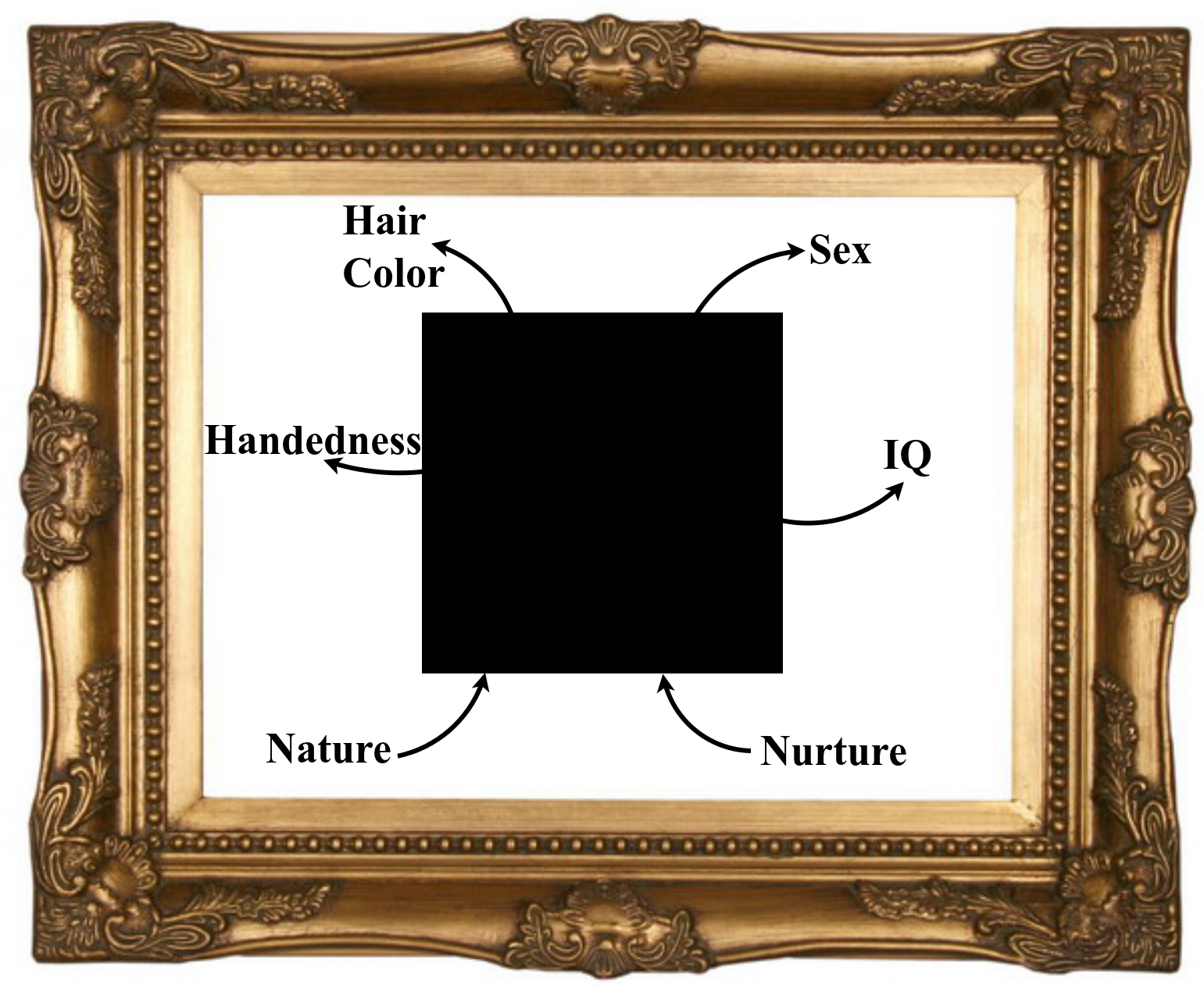
Contingency Tables
The $2\times 2$ table is most common:
| Blonde | Brunette | Totals | |
|---|---|---|---|
| Female | 18 | 17 | 35 |
| Male | 11 | 14 | 25 |
| Totals | 29 | 31 | 60 |
But doesn't this approach ignore the underlying biology?
Yes!
Contingency Tables

Contingency Tables
Contingency Tables

Contingency Tables
Contingency Tables
Contingency Tables
Fuel Cycle Contingency Tables
For example, let's construct a 2D contingency table that measures the response from a sample input: fast reactor fuel plutonium separation efficiency, FR_SE_PU.
$0.9<$SE$<0.99$ | $0.99<$SE$<0.999$ | $0.999<$SE$<0.9999$ | ||
|---|---|---|---|---|
$10^4 <$ Capacity $< 10^5$ | $739$ | $43$ | $27$ | $809$ |
$10^5 <$ Capacity $< 10^6$ | $31510$ | $21611$ | $19469$ | $72590$ |
$10^6 <$ Capacity $< 10^7$ | $2648$ | $13095$ | $14430$ | $30173$ |
$10^7 <$ Capacity $< 10^8$ | $0$ | $213$ | $1053$ | $1266$ |
| $34897$ | $34962$ | $34979$ | $104838$ |
Contingency Table Statistics
There are several metrics that have been developed to measure associations with contingency tables.
The primary measure here is the Uncertainty Coefficient $U(x|R)$.
To calculate $U(x|R)$ the following are needed:
- The Entropy $H(x)$, which is a measure of how evenly the data is spread out in the $x$ parameter.
- The Mutual Information $I(R,x)$ which states the shared value of the $x$ together with $R$.
Contingency Table Statistics
Denote the entries in a contingency table as $N_{ij}$ for the $i$-th response bin and the $j$-th input bin.
The probability of landing in a given bin is therefore,
Thus the entropy is calculated from,
The mutual information is found via,
Visual Relationship

Figure 11: Entropy Relations [4]
Contingency Table Statistics
The uncertainty coefficient is then calculated from,
This metric has the following useful properties:
- Defined on the range $[0, 1]$.
- $U(x|R) = 0$ implies that $I(R,x) = 0$, which indicates that the parameter is unassociated with the response.
- $U(x|R) = 1$ requires that $I(R,x) = H(x)$. This implies that the system response $R(x)$ is solely determined by $x$.
Input Parameters Ranked by $U(x|R)$
| Rank | $x$ | $U(x|R)$ |
|---|---|---|
| 1 | FR_SE_PU | 0.07667 |
| 2 | HLW_Storage_Time | 0.05264 |
| 3 | FR_SE_AM | 0.04148 |
| 4 | Heat_Loss_Factor | 0.01548 |
| 5 | LWR_SE_PU | 0.01343 |
| 6 | FR_TRU_CR | 0.008895 |
| 7 | LWR_SE_AM | 0.007304 |
| 8 | FR_BUd | 0.003773 |
| 9 | LWR_UF_Storage_Time | 0.003551 |
| 10 | Rock_Specific_Heat | 0.003085 |
| 11 | FR_SE_CM | 0.002522 |
| 12 | Rock_Thermal_Conductivity | 0.001954 |
| 13 | Ambient_Temp | 0.001353 |
| 14 | LWR_BUd | 0.001053 |
| 15 | LWR_SE_CS | 0.001033 |
Input Parameters Ranked by $U(x|R)$
| Rank | $x$ | $U(x|R)$ |
|---|---|---|
| 16 | LWR_SE_SR | 0.001024 |
| 17 | FR_UF_Storage_Time | 0.0005559 |
| 18 | Drift_Space | 0.0004421 |
| 19 | LWR_SE_U | 0.0002899 |
| 20 | Rock_Density | 0.0002718 |
| 21 | FR_SE_CS | 0.0001331 |
| 22 | FR_SE_SR | 0.0001073 |
| 23 | Vent_System_On_Time | 0.0001016 |
| 24 | Drift_Diameter | 9.648E-05 |
| 25 | LWR_SE_NP | 9.575E-05 |
| 26 | LWR_SE_CM | 7.969E-05 |
| 27 | LWR_Fuel2Mod | 7.833E-05 |
| 28 | FR_LAN_FF_Cap | 6.559E-05 |
| 29 | FR_SE_NP | 6.212E-05 |
| 30 | FR_SE_U | 6.207E-05 |
$U(x|R)$ Rankings vs $U(R|x)$ Rankings
$U(x|R)$ is related to $U(R|x)$ via the following expression:
This is effectively an entropic re-expression of Bayes' Theorem:
Due to the stochastic driver, all $H(x)$ must be the same - to within error - for all $x$. Also, since there is only one repsonse, $H(R)$ is the same the for all $x$.
Hence, $U(x|R) = k U(R|x)$.
Scaling the uncertainty coefficients by a constant does not affect the relative rank ordering.
Entropy Based Covariance
- Now that the association of $x$ to $R$ may be determined, finding the sensitivity of $R(x)$ to other inputs.
- Call $y$ an input parameter distinct from $x$. Measuring the simultaneous effect of two inputs to a response may be performed using 3D tables!
- Note that 'slices' of these 3D tables may be seen as 2D tables bins along a specific cut of data.
- For 30 inputs, there are $_{30}C_2 = 435$ contingency tables to construct.
- Different metrics will be needed to account for the added dimensionality.
FR Pu SE and HLW Storage Time
Slice for 1 < HLW_Storage_Time < 6.694
$0.9<$SE$<0.99$ | $0.99<$SE$<0.999$ | $0.999<$SE$< 0.9999$ | ||
|---|---|---|---|---|
$10^4 <$ Capacity $< 10^5$ | $419$ | $23$ | $14$ | $456$ |
$10^5 <$ Capacity $< 10^6$ | $11145$ | $9970$ | $9553$ | $30668$ |
$10^6 <$ Capacity $< 10^7$ | $110$ | $1556$ | $2085$ | $3751$ |
$10^7 <$ Capacity $< 10^8$ | $0$ | $0$ | $0$ | $0$ |
| $11674$ | $11549$ | $11652$ | $34875$ |
Slice for 6.694 < HLW_Storage_Time < 44.814
$0.9<$SE$<0.99$ | $0.99<$SE$<0.999$ | $0.999<$SE$< 0.9999$ | ||
|---|---|---|---|---|
$10^4 <$ Capacity $< 10^5$ | $273$ | $19$ | $11$ | $303$ |
$10^5 <$ Capacity $< 10^6$ | $10859$ | $7527$ | $6373$ | $24759$ |
$10^6 <$ Capacity $< 10^7$ | $484$ | $4157$ | $5175$ | $9816$ |
$10^7 <$ Capacity $< 10^8$ | $0$ | $2$ | $24$ | $26$ |
| $11616$ | $11705$ | $11583$ | $34904$ |
FR Pu SE and HLW Storage Time
Slice for 44.814 < HLW_Storage_Time < 300
$0.9<$SE$<0.99$ | $0.99<$SE$<0.999$ | $0.999<$SE$< 0.9999$ | ||
|---|---|---|---|---|
$10^4 <$ Capacity $< 10^5$ | $47$ | $1$ | $2$ | $50$ |
$10^5 <$ Capacity $< 10^6$ | $9506$ | $4114$ | $3543$ | $17163$ |
$10^6 <$ Capacity $< 10^7$ | $2054$ | $7382$ | $7170$ | $16606$ |
$10^7 <$ Capacity $< 10^8$ | $0$ | $211$ | $1029$ | $1240$ |
| $11607$ | $11708$ | $11744$ | $35059$ |
Aggregation over HLW_Storage_Time
$0.9<$SE$<0.99$ | $0.99<$SE$<0.999$ | $0.999<$SE$< 0.9999$ | ||
|---|---|---|---|---|
$10^4 <$ Capacity $< 10^5$ | $739$ | $43$ | $27$ | $809$ |
$10^5 <$ Capacity $< 10^6$ | $31510$ | $21611$ | $19469$ | $72590$ |
$10^6 <$ Capacity $< 10^7$ | $2648$ | $13095$ | $14430$ | $30173$ |
$10^7 <$ Capacity $< 10^8$ | $0$ | $213$ | $1053$ | $1266$ |
| $34897$ | $34962$ | $34979$ | $104838$ |
Covariance Statistics
- While $U(x,y|R)$ is roughly equivalent to the concept of mutual sensitivity, 3D tables should allow for an information theoretic parallel to covariance.
- In general for contingency tables covariance is not well defined, however here there is the special stochastic situation where $x$ and $y$ are known a priori to be independent of $R$.
- Therefore, the following new coefficient of variation metric is proposed.
- $c_v(x|y|R)$ is the 'sensitivity of sensitivity', or how much an input affects the response of another input.
Covariance Statistics
First, define:
Then the coefficient of variation is,
Finally, the symmetric $c_v$ is set as:
Covariance Statistics
$c_v(x|y|R)$ has the following properties:
- Defined on the range $[0, 1]$ since $0 \le U \le 1$.
- $c_v = 0$ implies that $\sigma = 0$, which indicates that $U(x|R)$ shows no association with $y$. Thus there are no covariant effects observed.
- $c_v = 1$ indicates that $\sigma = \mu$. This connotes that the value of $x$ solely governs the response $R$ from $y$.
Top Covariant Parameter Pair Rankings
| Rank | $x$ | $y$ | $c_v(x|y|R)$ |
|---|---|---|---|
| 1 | FR_SE_AM | HLW_Storage_Time | 0.02318 |
| 2 | FR_SE_AM | FR_SE_PU | 0.02316 |
| 3 | HLW_Storage_Time | LWR_UF_Storage_Time | 0.01557 |
| 4 | FR_SE_PU | HLW_Storage_Time | 0.01556 |
| 5 | HLW_Storage_Time | LWR_SE_PU | 0.01155 |
| 6 | FR_SE_AM | FR_TRU_CR | 0.01061 |
| 7 | FR_SE_PU | LWR_UF_Storage_Time | 0.008192 |
| 8 | FR_SE_PU | LWR_SE_PU | 0.008 |
| 9 | FR_BUd | FR_SE_AM | 0.007716 |
| 10 | Ambient_Temp | FR_SE_PU | 0.007489 |
| 11 | Ambient_Temp | HLW_Storage_Time | 0.007367 |
| 12 | HLW_Storage_Time | LWR_SE_AM | 0.007248 |
| 13 | Ambient_Temp | FR_SE_CS | 0.007235 |
| 14 | Ambient_Temp | LWR_Fuel2Mod | 0.007066 |
| 15 | Ambient_Temp | Heat_Loss_Factor | 0.007044 |
Covariant Parameter Pair Example

Figure 11: Total & Top Contributors to Decay Heat [Watts/kg] of HLW for (FR_SE_AM, FR_SE_PU).
Ensuring Good Statistics
How do we know that we have picked a sufficient number of bins?
Different partitioning schemes may significantly alter our measures. Consider a a chamber the moment after a piston has been suddenly removed, as in a Carnot heat engine:

Figure 12: Abstract Piston with Representative Partitions: Blue Line for 2 Bins, Red Line for 5 Bins.
Ensuring Good Statistics
We thus want to pick the minumum number of bins after which our metrics (and rankings) have stablized.

Figure 13: Dynamic Effects of Binning Structure Example: $U(x,y|R)$ for the parameter pair (FR_SE_PU, LWR_SE_NP) to repository capacity.
Ensuring Good Statistics
But how many runs are needed to achieve this binning?
For the covariance measures (which determines the statistics), note that:
Set $t$ as a fractional statistical tolerance, ie $t=0.01$ is 1% error.
Then the mutual information goes as $I = t^d$ for $d$ indpendent inputs. Here, $d = 2$ for $x$ & $y$.
For $J$ number $x$ bins and $K$ number of $y$ bins, the total number of runs required is estimated by:
Obligatory Open Source Rant (Do it! Do it now!)
![]() - PyNE, Cyclus, OpenMC, Fudge, Software Carpentry, etc.
- PyNE, Cyclus, OpenMC, Fudge, Software Carpentry, etc.
 - June 24th - 29th, Austin, TX! http://conference.scipy.org/scipy2013/
 - http://numfocus.org/
Questions

References
- Anthony M. Scopatz and Erich a. Schneider. “A new method for rapid computation of transient fuel cycle material balances”. In: Nuclear Engineering and Design 239.10 (Oct. 2009), pp. 2169–2184. ISSN: 00295493. DOI: 10.1016/j.nucengdes.2009.02.022. URL: http://linkinghub.elsevier.com/retrieve/pii/S0029549309000922
- M Takano. Burnup Credit Criticality Benchmark - Result of Phase 1A - NEA/NSC/DOC(93)22. Tech. rep. January. Nuclear Energy Agency, 1994, pp. 1–147
- OECD. Advanced Nuclear Fuel Cycles and Radioactive Waste Management - NEA-5990. Tech. rep. Nuclear Energy Agency, 2006, pp. 1–248
- http://en.wikipedia.org/wiki/File:Entropy-mutual-information-relative-entropy-relation-diagram.svg
- Nuclear Energy Data Files. Los Alamos National Laboratory - Theoretical Nuclear Physics. 2009. URL: http://t2.lanl.gov/data/data.html
- Jaakko Lepp. PSG2 / Serpent âA ̧ a Continuous-energy Monte Carlo Reactor Physics Burnup Calculation Code. Tech. rep. 2011, p. 157
- A G Croff. ORIGEN 2.2 - CCC-371. Tech. rep. Oak Ridge National Laboratory, 2002, pp. 1–222