6-raster-data

background-size: cover

<h1 class="center middle">Raster Data and the {raster} package</h1>

---

# The `raster` package is 10 years old!

![:imgcenterscale 50%](images/section-6/old.gif)

---

# But it has been around for so long for a reason

* It's powerful

* It's intuitive (at least I think so)

* Robert keeps it up to date

---

# Robert J. Hijmans

![:imgcenterscale 50%](images/section-6/robert_hijmans.jpg)

---

# Fully updated intro vignette

[This is a useful reference.](https://cran.r-project.org/web/packages/raster/vignettes/Raster.pdf)

---

# As discussed earlier, "raster" refers to gridded data

---

# And raster data can be single-band or multiple-band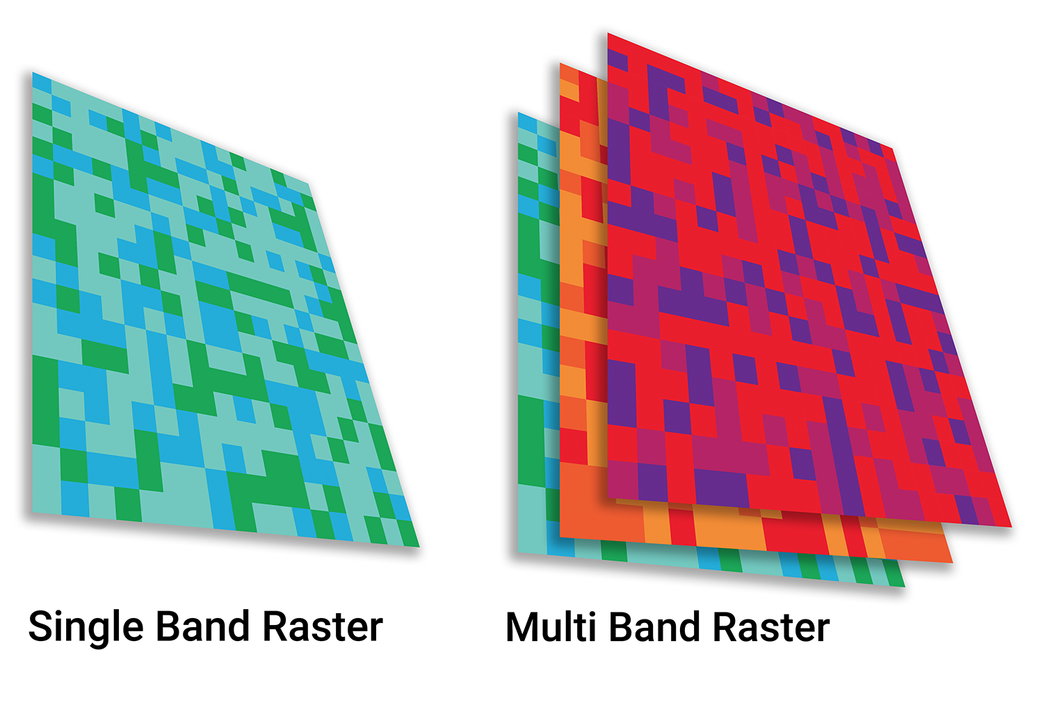

![:imgcenterscale 90%](images/section-2/single_multi_raster-sara.png)

---

# Read a single-band raster with `raster()`

```r
elevation <- raster("data/elevation.tif", quiet = TRUE)
```

---

# Single-band class is `RasterLayer`

```r
class(elevation)
```

```
## [1] "RasterLayer"
## attr(,"package")
## [1] "raster"
```

---

# Map the elevation data

```r
tm_shape(elevation) + 
  tm_raster()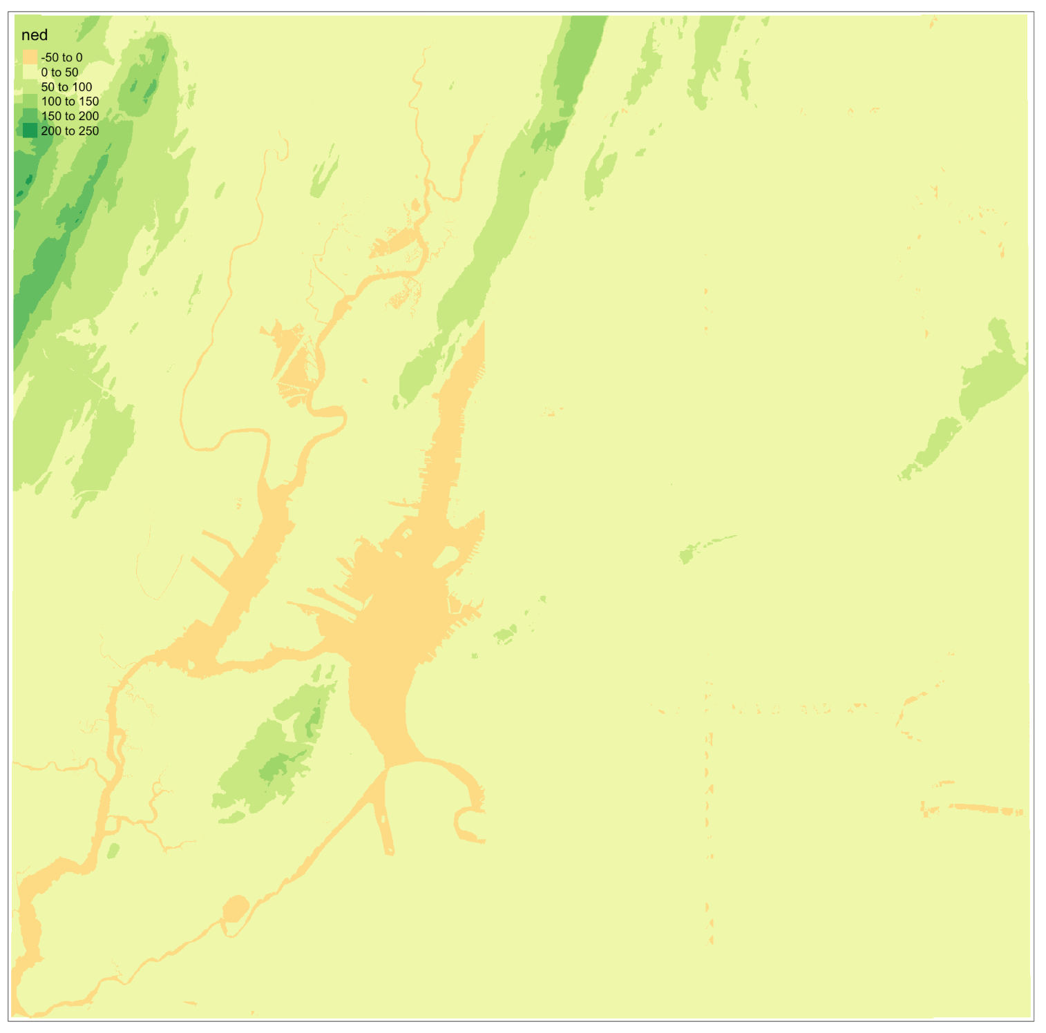 
```

![:imgcenterscale 50%](images/section-6/ned_highres.png)

---

# Our `RasterLayer` metadata

```r
elevation
```

```
## class      : RasterLayer 
## dimensions : 1530, 2039, 3119670  (nrow, ncol, ncell)
## resolution : 77, 101  (x, y)
## extent     : 911860, 1068863, 119161.4, 273691.4  (xmin, xmax, ymin, ymax)
## crs        : +proj=lcc +lat_1=41.03333333333333 +lat_2=40.66666666666666 +lat_0=40.16666666666666 +lon_0=-74 +x_0=300000.0000000001 +y_0=0 +ellps=GRS80 +towgs84=0,0,0,0,0,0,0 +units=us-ft +no_defs 
## source     : /Volumes/GoogleDrive/My Drive/projects/workshop-r-spatial-slides/big-project-files/gis-data/nyc/processed/ned.tif 
## names      : ned 
## values     : -14.05926, 209.7131  (min, max)
```

---

# Read a multi-band raster with `brick()`

```r
satellite_image <- brick("data/satellite.tif", quiet = TRUE)
```

---

# Multi-band class is `RasterBrick`

```r
class(satellite_image)
```

```
## [1] "RasterBrick"
## attr(,"package")
## [1] "raster"
```

---

# Map multi-band raster with `tm_raster()`

This is an image raster with a red, green and blue layer. What happens here?

```r
tm_shape(satellite_image) + tm_raster()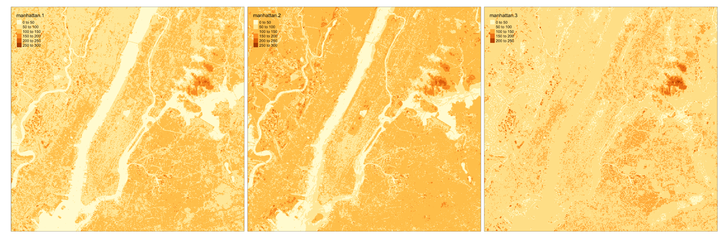
```

--
![:imgcenterscale 100%](images/section-6/multi_each_band.png)

---

# Map our multi-band image with `tm_rgb()`

```r
tm_shape(satellite_image) + tm_rgb()
```

---

# The metadata in a `RasterBrick` object is very similar

```r
satellite_image
```

```
## class      : RasterBrick 
## dimensions : 773, 801, 619173, 3  (nrow, ncol, ncell, nlayers)
## resolution : 29.98979, 30.00062  (x, y)
## extent     : 575667.9, 599689.7, 4503277, 4526468  (xmin, xmax, ymin, ymax)
## crs        : +proj=utm +zone=18 +datum=WGS84 +units=m +no_defs +ellps=WGS84 +towgs84=0,0,0 
## source     : /Users/zevross/git-repos/workshop-r-spatial-slides/data/nyc/manhattan.tif 
## names      : manhattan.1, manhattan.2, manhattan.3 
## min values :           0,           0,           0 
## max values :         255,         255,         255
```

---

# Get the names of your layers with `names()`

```r
names(satellite_image)
```

```
## [1] "manhattan.1" "manhattan.2" "manhattan.3"
```

---

# Two options for extracting a layer of your brick

```r
satellite_image$manhattan.1
```

```r
subset(satellite_image, "manhattan.1")
```

---

exclude:true

# RasterStack

???

The principal difference between these two classes is that a RasterBrick can only be linked to a single (multi-layer) file. In contrast, a RasterStack can be formed from separate files and/or from a few layers (‘bands’) from a single file.In fact, a RasterStack is a collection of RasterLayer objects with the same spatial extent and resolution. In essence it is a list of RasterLayer objects. A RasterStack can easily be formed form a collection of files in different locations and these can be mixed with RasterLayer objects that only exist in the RAM memory (not on disk).A RasterBrick is truly a multi-layered object, and processing a RasterBrick can be more efficient than processing a RasterStack representing the same data. However, it can only refer to a single file. A typical example of such a file would be a multi-band satellite image or the output of a global climate model (with e.g., a time series of temperature values for each day of the year for each raster cell). Methods that operate on RasterStack and RasterBrick objects typically return a RasterBrick object.

---

# You can also use `raster()` and `brick()` to create a raster from scratch

---

# Create a boring raster

```r
r <- raster(nrow = 10, ncol = 10)
```

---

# Try to plot your boring raster

```r
plot(r)
```

```
## Error in .plotraster2(x, col = col, maxpixels = maxpixels, add = add, : no values associated with this RasterLayer
```

---

# Why no plot?

---

# Use the `getValues()` function to look at the values

```r
getValues(r)
```

```
##   [1] NA NA NA NA NA NA NA NA NA NA NA NA NA NA NA NA NA NA NA NA NA NA NA
##  [24] NA NA NA NA NA NA NA NA NA NA NA NA NA NA NA NA NA NA NA NA NA NA NA
##  [47] NA NA NA NA NA NA NA NA NA NA NA NA NA NA NA NA NA NA NA NA NA NA NA
##  [70] NA NA NA NA NA NA NA NA NA NA NA NA NA NA NA NA NA NA NA NA NA NA NA
##  [93] NA NA NA NA NA NA NA NA
```

---

# Can't plot a raster with no values

---

# Use `values()` to add values

```r
values(r) <- rnorm(100) # assign random normal data
```

```r
# You can also include values when creating
r <- raster(nrow = 10, ncol = 10, vals = rnorm(100))
```

---

# Now we can plot

```r
plot(r, axes = FALSE)
```

---

# Note that your cell values cannot be characters

```r
my_letters <- sample(LETTERS, 100, replace = TRUE)
head(my_letters)
```

```
## [1] "R" "Q" "C" "X" "D" "K"
```

```r
values(r) <- my_letters
```

```
## Error in setValues(x, value): values must be numeric, integer, logical or factor
```

---

# But they can be factors

```r
values(r) <- factor(my_letters)
```

```r
tm_shape(r) + tm_raster()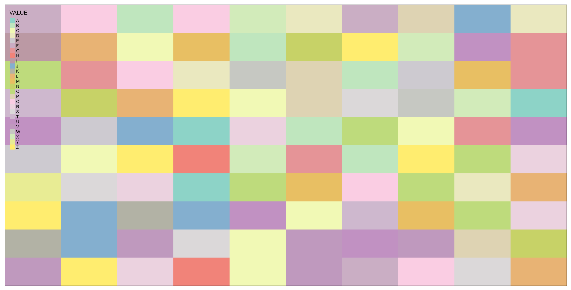
```
![:imgcenterscale 100%](images/section-6/letters.png)

---

# Technically the values stored are integers mapped to a table of levels

```r
getValues(r)[1:10]
```

```
##  [1] 18 17  3 24  4 11  1  5 22 19
```

---

# The levels of the categorical raster can be accessed with `levels()`

```r
levels(r)[[1]][1:5,]
```

```
##   ID VALUE
## 1  1     A
## 2  2     B
## 3  3     C
## 4  4     D
## 5  5     E
```

---

# A brick can be created by stacking `RasterLayers` with `brick()`

---

# Perhaps the most boring brick ever created...

```r
b <- brick(r, r, r)
b
```

```
## class      : RasterBrick 
## dimensions : 10, 10, 100, 3  (nrow, ncol, ncell, nlayers)
## resolution : 36, 18  (x, y)
## extent     : -180, 180, -90, 90  (xmin, xmax, ymin, ymax)
## crs        : +proj=longlat +datum=WGS84 +ellps=WGS84 +towgs84=0,0,0 
## source     : memory
## names      : layer.1, layer.2, layer.3 
## min values :       1,       1,       1 
## max values :      26,      26,      26
```

---

# Where, on earth, are those rasters we just created?

---

# By default, those hand-created rasters span the globe

And have an unprojected CRS of WGS84

---

# To prove this, read in the countries with {rnaturalearth} for context

```r
countries <- rnaturalearth::ne_countries()
```

---

# Map our random letters raster with countries on top

```r
tm_shape(r) + tm_raster(alpha = 0.5) + 
  tm_shape(countries) + tm_borders(lwd=2)
```

![:imgcenterscale 100%](images/section-6/world_manual_raster.png)

---

# But if you want your raster in a specific place on earth

---

# You can use another object to define the extent

```r
boroughs <- read_sf("boroughs.gpkg")
```

---

# Supply the object to `raster()`

```r
rand <- raster(boroughs, ncols = 10, nrows = 10, 
               vals = rnorm(100))
```

---

# Plot our random raster

```r
tm_shape(rand) + 
  tm_raster(n = 100, legend.show = FALSE) + 
  tm_shape(boroughs) + 
  tm_borders(lwd = 3, col = "black")
```

---

# Extracting information about your rasters

---

# The console printout shows the metadata

```r
elevation
```

---

# You can access the "slots" (attributes) directly

```r
elevation@crs
```

```
## CRS arguments:
##  +proj=lcc +lat_1=41.03333333333333 +lat_2=40.66666666666666
## +lat_0=40.16666666666666 +lon_0=-74 +x_0=300000.0000000001 +y_0=0
## +ellps=GRS80 +towgs84=0,0,0,0,0,0,0 +units=us-ft +no_defs
```

```r
elevation@data@max
```

```
## [1] 209.7131
```

---

# But there are utility functions to make it easier

```r
crs(elevation)
```

```r
maxValue(elevation)
```

```
## [1] 209.7131
```

---

# Many more useful utility functions

* `extent()`
* `ncell()`
* `nlayers()`
* `filename()`
* `crs()`
* `minValue()`

---

# Get cell value counts with `freq()`

```r
r <- raster(nrow = 100, ncol = 100, 
            vals = sample(1:10, 100*100, replace = TRUE))
```

```r
freq(r) %>% 
  head()
```

```
##      value count
## [1,]     1  1071
## [2,]     2   980
## [3,]     3   981
## [4,]     4  1006
## [5,]     5   981
## [6,]     6   986
```

---

# {raster} can work with large rasters

---

# The elevation raster has a lot of grid cells

```r
ncell(elevation)
```

```
## [1] 3119670
```

---

# More than 3 million cells but in R it takes little memory

```r
pryr::object_size(elevation)
```

```
## 11.6 kB
```

---

# On disk, the file is not small

```r
# Size on my computer
fs::file_info("elevation.tif")$size
```

```
## 10.2M
```

---

# Raster values are not read by default

* Rasters can be very big

* To conserve memory raster values are imported only when required

* For large rasters, data is processed in chunks

---

## The `inMemory()` function tells you if the raster values have been read into R

```r
inMemory(satellite_image)
```

```
## [1] FALSE
```

---

## Read values with the `getValues()` function

```r
vals <- getValues(elevation)
hist(vals)
```

---

# Converting between vectors and rasters

---

# Note that while there is some support for {sf} in {raster} it is not complete

---

# You'll need to review the function documentation to determine what type of input is accepted

---

# If a function only accepts a `Spatial*` object you can convert with `as()`

```r
class(boroughs)
```

```
## [1] "sf"         "tbl_df"     "tbl"        "data.frame"
```
--

```r
as(boroughs, "Spatial") %>% class()
```

```
## [1] "SpatialPolygonsDataFrame"
## attr(,"package")
## [1] "sp"
```

---

# Use the `rasterize()` function to convert vectors to raster

.footnote[For large rasters this can be computationally intensive and the {fasterize} package can help speed things up]

---

# You might do this for landscape analysis or raster math

![:imgcenterscale 50%](images/section-6/rastermath.png)

---

# With `rasterize()` you assign the attributes from a vector layer to a raster

---

# For this example we will create a raster layer of the boroughs

---

# Our boroughs vector data

```r
tm_shape(boroughs) + tm_polygons("BoroName")
```

<img src="6-raster-data_files/figure-html/unnamed-chunk-50-1.svg" style="display: block; margin: auto;" />
---

# Our boroughs attribute table

```r
glimpse(boroughs)
```

```
## Observations: 5
## Variables: 7
## $ BoroCode   <int> 1, 2, 5, 3, 4
## $ BoroName   <chr> "Manhattan", "The Bronx", "Staten…
## $ Shape_Leng <dbl> 339736.6, 397460.6, 318700.5, 576…
## $ Shape_Area <dbl> 635147797, 1182399343, 1630762350…
## $ diso       <int> 1, 1, 1, 1, 1
## $ AreaSqMile <dbl> 22.78279, 42.41274, 58.49555, 71.…
## $ geom       <MULTIPOLYGON [US_survey_foot]> MULTIPO…
```

---

# Step 1: Convert to an {sp} object

After reviewing the help for `rasterize()`

```r
boroughs_sp <- as(boroughs, "Spatial")
```

---

# Step 2: create the raster that values will be transferred to

```r
n <- 1000
r <- raster(boroughs_sp, ncols = n, nrows = n)
```

---

# Run `rasterize()`

```r
boro_raster <- rasterize(boroughs_sp, r, field = "BoroCode")
```

---

# Our rasterized boroughs

```r
tm_shape(boro_raster) + tm_raster() + tm_layout(legend.show = FALSE)
```

---

# For converting from a raster to vectors you can use

* `rasterToPolygons()`
* `rasterToPoints()`

---

# Create a random raster for this example

```r
set.seed(100)
r <- raster(nrow = 30, ncol = 30, 
            vals = sample(1:3, 900, replace = TRUE))
```

```r
tm_shape(r) + tm_raster() + tm_layout(legend.show = FALSE)
```
![:imgcenterscale 100%](images/section-6/random_for_to_vector.png)

---

# Extract points from the raster

As a Spatial* object with `spatial = TRUE`

```r
pts <- rasterToPoints(r, spatial = TRUE)
```

```r
class(pts)
```

```
## [1] "SpatialPointsDataFrame"
## attr(,"package")
## [1] "sp"
```

---

# Convert to an {sf} object

```r
pts <- as(pts, "sf")
```

```r
# This also works
pts <- st_as_sf(pts)
```

---

# Plot the points

```r
my_layout <-   tm_layout(frame = FALSE, legend.show = FALSE)
m1 <- tm_shape(r) + tm_raster() + my_layout
m2 <- tm_shape(pts) + tm_dots("layer", size = 0.5, shape = 21) + my_layout
tmap_arrange(m1, m2, nrow = 1)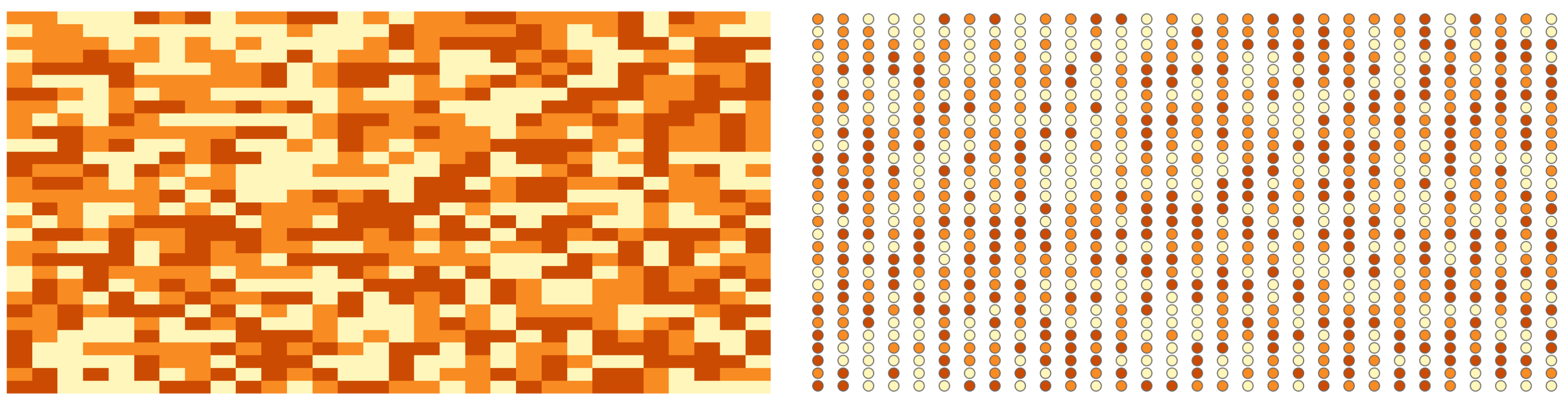
```

![:imgcenterscale 100%](images/section-6/raster_and_points.png)

---

# Extract the polygons

```r
polys <- rasterToPolygons(r, dissolve = TRUE) %>% 
  st_as_sf(sf)
```

---

# Plot the polys

```r
m3 <- tm_shape(polys) + 
  tm_polygons("layer", border.col = "black") + my_layout
tmap_arrange(m1, m3, nrow = 1)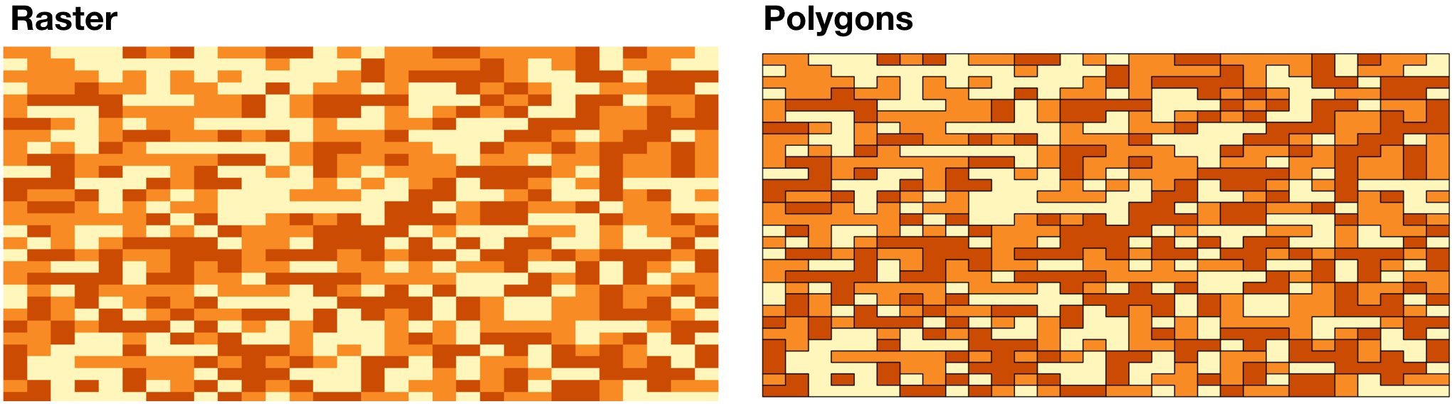
```

![:imgcenterscale 100%](images/section-6/raster_to_polygons.png)
---
class: center, middle, doExercise

# open_exercise(6)