class: title-slide background-size: cover <h1 class="center middle">Vector Data and the <br> {sf} Package</h1> <h3 class="center middle"></h3> <div class="logo"></div> <div class="databird"></div> --- # In the beginning there was {sp} 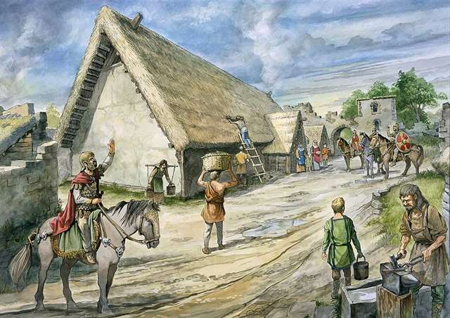 --- # It was powerful and it worked but... --- # Spatial analysis was more challenging with {sp} -- * Didn't integrate as well with non-spatial data -- * The many different spatial classes were confusing ```r sp::SpatialPoints() sp::SpatialPointsDataFrame() sp::SpatialGrid() sp::SpatialGridDataFrame() sp::SpatialPixels() sp::SpatialPixelsDataFrame() ``` --- # The code did not come naturally  --- # Then there was {sf}  --- # OK it can still be a challenge  --- class: center, middle # A little about {sf} --- # The {sf} package has made my work life easier {sf} stands for "simple features", a standardized way to encode spatial vector data --- # "sf" stands for simple features The "simple" in simple features refers to representing lines and polygons based on sequences of points connected by straight lines. --- # Authors of {sf} .pull-left[  Edzer Pebesma ] .pull-left[  Roger Bivand ] --- # Edzer and Roger also created {sp}, the pre-cursor to {sf} * Initial release of {sf} was at the end of 2016 * Before that, {sp} goes back to 2005 --- # Two references * [Edzer's book on spatial data science](https://keen-swartz-3146c4.netlify.com/) is still being developed. * The [R Journal article](https://journal.r-project.org/archive/2018/RJ-2018-009/RJ-2018-009.pdf) on `sf` --- # You can't completely ignore {sp} * Some packages have not been updated to use {sf} classes --- # {sf} is not stand-alone R code * Depends on C/C++ libraries * GDAL: for reading and writing data * GEOS: for geometric operations (e.g., union, intersects etc) * PROJ: for CRS support --- # You see these dependencies when you load {sf}! --  --- # If you only work with vector data you may not need any other package --- # Functions in {sf} generally start with `st_` Referring to "spatial type" ```r st_buffer() st_intersection() st_centroid() ``` --- # The beauty of {sf} is that spatial objects are just special data frames --- background-image: url("images/rworkshop_divider.png") background-size: cover class: center, middle, separator-slide # What is a simple features data frame in R? --- # Short answer is - a data frame with a geometry column --- # Longer answer with example --- # Read in geographic data as {sf} data frame ```r boroughs <- read_sf("boroughs.gpkg") ``` --- # Here's what the data look like as a map ```r tm_shape(boroughs) + tm_polygons("BoroName") ``` <img src="5-vector-data_files/figure-html/unnamed-chunk-5-1.svg" style="display: block; margin: auto;" /> --- # Here's what the data look like with `glimpse()` ```r glimpse(boroughs) ``` ``` ## Observations: 5 ## Variables: 4 ## $ BoroCode <int> 1, 2, 5, 3, 4 ## $ BoroName <chr> "Manhattan", "The Bronx", "Staten… ## $ AreaSqMile <dbl> 22.78279, 42.41274, 58.49555, 71.… ## $ geom <MULTIPOLYGON [°]> MULTIPOLYGON (((-73.… ``` --- # Look at the data with `head()` ```r head(boroughs) ``` ``` ## Simple feature collection with 5 features and 3 fields ## geometry type: MULTIPOLYGON ## dimension: XY ## bbox: xmin: -74.25589 ymin: 40.49593 xmax: -73.70001 ymax: 40.91577 ## epsg (SRID): 4326 ## proj4string: +proj=longlat +datum=WGS84 +no_defs ## # A tibble: 5 x 4 ## BoroCode BoroName AreaSqMile geom ## <int> <chr> <dbl> <MULTIPOLYGON [°]> ## 1 1 Manhattan 22.8 (((-73.91839 40.86014, -73.9184 40.8601, … ## 2 2 The Bronx 42.4 (((-73.78756 40.87256, -73.78723 40.87237… ## 3 5 Staten Is… 58.5 (((-74.05675 40.6081, -74.05664 40.608, -… ## 4 3 Brooklyn 71.5 (((-73.98569 40.5813, -73.98368 40.58303,… ## 5 4 Queens 110. (((-73.70089 40.74706, -73.70078 40.74504… ``` --- # Geometry column is usually called `geometry` or `geom` ``` ## Observations: 5 ## Variables: 4 ## $ BoroCode <int> 1, 2, 5, 3, 4 ## $ BoroName <chr> "Manhattan", "The Bronx", "Staten… ## $ AreaSqMile <dbl> 22.78279, 42.41274, 58.49555, 71.… ## $ geom <MULTIPOLYGON [°]> MULTIPOLYGON (((-73.… ``` --- # The class of the full dataset is `sf` And it is also a data frame and might be a tibble (a tidyverse data frame) -- ```r class(boroughs) ``` ``` ## [1] "sf" "tbl_df" "tbl" "data.frame" ``` .footnote[ The tibble class will not be added if you read with `st_read()`. ] --- # But what is the geometry column? -- ```r # These will give the same result boroughs$geom st_geometry(boroughs) ``` ``` ## Geometry set for 5 features ## geometry type: MULTIPOLYGON ## dimension: XY ## bbox: xmin: -74.25589 ymin: 40.49593 xmax: -73.70001 ymax: 40.91577 ## epsg (SRID): 4326 ## proj4string: +proj=longlat +datum=WGS84 +no_defs ``` --- # The class for the geometry is `sfc` This is a simple features list column. -- ```r class(boroughs$geom) ``` ``` ## [1] "sfc_MULTIPOLYGON" "sfc" ``` --- # One list element for each geometry/feature So how many list items are there in this dataset? ```r length(boroughs$geom) ``` -- ``` ## [1] 5 ``` --- # Print out the first geometry from the list-column ```r one_geometry <- boroughs$geom[[1]] ``` -- ```r one_geometry ``` 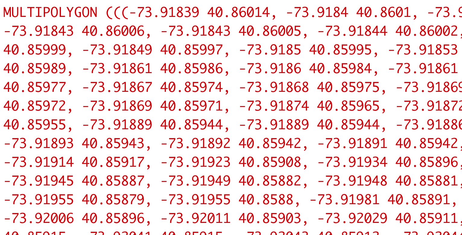 .footnote[ Abbreviated output ] --- # Trick question: what is the result of this? ```r length(one_geometry) ``` -- ``` ## [1] 19 ``` --- # One borough but 19 little pieces A "MULTIPOLYGON" ```r plot(one_geometry) ``` 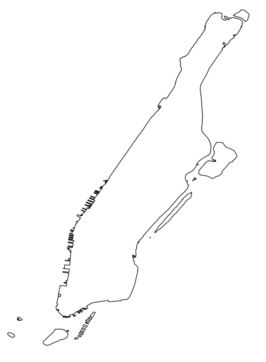 --- # The class of this one geometry is `sfg` "Simple features geometry" -- ```r class(one_geometry) ``` ``` ## [1] "XY" "MULTIPOLYGON" "sfg" ``` --- # Seven main feature types For representing a single feature  --- # You *can* create `sfg` objects manually ```r pt_sfg <- st_point(c(-122.431297, 37.773972)) ``` -- ```r class(pt_sfg) ``` ``` ## [1] "XY" "POINT" "sfg" ``` --- # But you rarely need to --- exclude: true # To convert the `sfg` to an `sf` data frame... -- exclude: true * First, you need to make it an `sfc` -- exclude: true * And then convert it to an `sf` data frame --- exclude: true # Geometry to `sf` process ```r pt_sfg <- st_point(c(-122.431297, 37.773972)) ``` -- exclude: true ```r # Geometry to geometry list column pt_sfc <- pt_sfg %>% st_sfc(crs = 4326) # accepts a crs ``` -- exclude: true ```r # Geometry list column to sf data frame pt_sf <- pt_sfc %>% st_sf() ``` --- exclude: true # Let's put it on a map --- exclude: true # First let's get the underlying county boundaries with {tigris} -- exclude: true ```r options(tigris_class = "sf") ca <- tigris::counties(state = "ca", resolution = "20m") ``` --- exclude: true # Create the map -- exclude: true ```r tm_shape(ca) + tm_polygons() + tm_shape(pt_sf) + tm_dots(size = 2, col = "red") ``` -- exclude: true 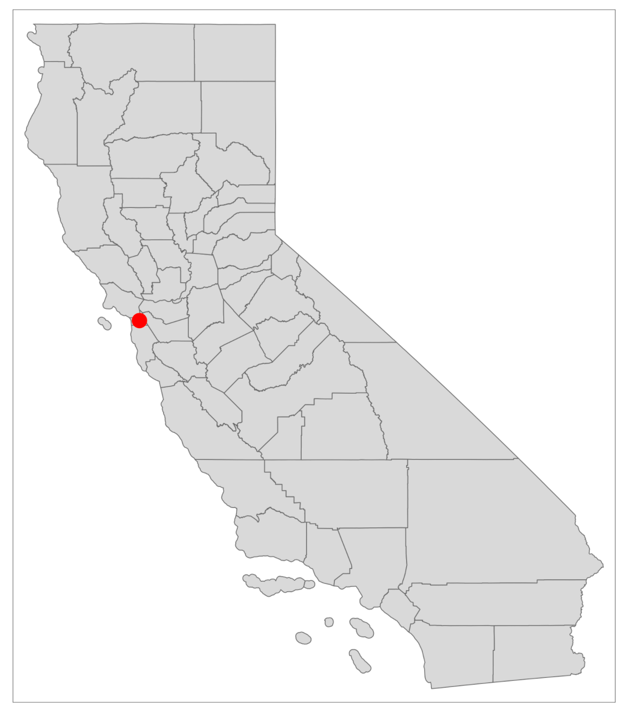 --- exclude: true # By the way `tmap` can't be used on an `sfg` object -- exclude: true ```r class(one_geometry) ``` ``` ## [1] "XY" "MULTIPOLYGON" "sfg" ``` -- exclude: true ```r # Error trying to map sfg tm_shape(one_geometry) + tm_polygons() ``` ``` ## Error in get_projection(mshp_raw, output = "crs"): shp is neither a sf, sp, nor a raster object ``` --- exclude: true # But you can use `plot()` on an `sfg` object ```r plot(one_geometry) ```  --- exclude: true # To reiterate -- exclude: true * `sf`: class of full dataset -- exclude: true * `sfc`: class of the list column in the dataset -- exclude: true * `sfg`: class of the individual geometries in the list column --- # A visual: `sf`, `sfc`, `sfg` 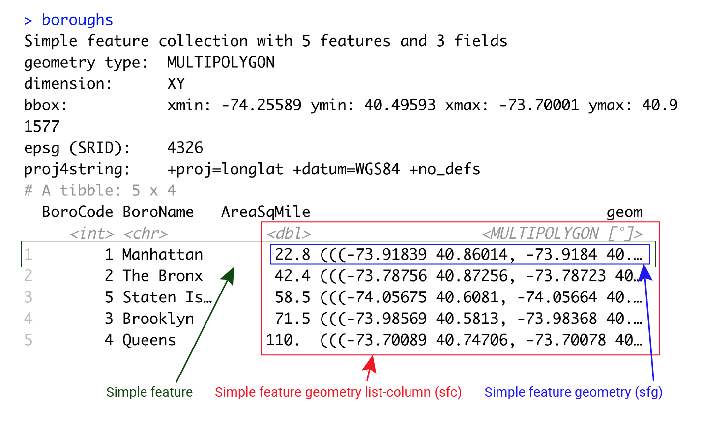 --- # Thankfully, most of what you will want to do uses {sf} data frames --- class: center, middle, doExercise # open_exercise(5) just do activities 1-5 --- background-image: url("images/background-old.jpg") background-size: cover class: center, middle, separator-slide # Manipulating your {sf} objects --- # You can use `dplyr` on your `sf` objects! --  --- # Read in NYC neighborhoods ```r neighborhoods <- read_sf("neighborhoods.shp") ``` -- ```r glimpse(neighborhoods) ``` ``` ## Observations: 195 ## Variables: 8 ## $ ntacode <chr> "BK88", "QN51", "QN27", "QN07", … ## $ shape_area <dbl> 5.0172283, 4.8763184, 1.8326831,… ## $ county_fips <chr> "047", "081", "081", "081", "061… ## $ ntaname <chr> "Borough Park", "Murray Hill", "… ## $ shape_leng <dbl> 11.962555, 10.139753, 6.040134, … ## $ boro_name <chr> "Brooklyn", "Queens", "Queens", … ## $ boro_code <chr> "3", "4", "4", "4", "1", "4", "3… ## $ geom <MULTIPOLYGON [US_survey_foot]> MULTIP… ``` --- # What if we only want neighborhoods in Brooklyn? -- And maybe drop a couple of columns --- # Use {dplyr} to filter and select -- ```r brooklyn <- neighborhoods %>% select(-shape_area, -shape_leng) %>% filter(boro_name == "Brooklyn") glimpse(brooklyn) ``` ``` ## Observations: 51 ## Variables: 6 ## $ ntacode <chr> "BK88", "BK25", "BK95", "BK69", … ## $ county_fips <chr> "047", "047", "047", "047", "047… ## $ ntaname <chr> "Borough Park", "Homecrest", "Er… ## $ boro_name <chr> "Brooklyn", "Brooklyn", "Brookly… ## $ boro_code <chr> "3", "3", "3", "3", "3", "3", "3… ## $ geom <MULTIPOLYGON [US_survey_foot]> MULTIP… ``` --- # Just Brooklyn ```r st_geometry(brooklyn) %>% plot() ``` 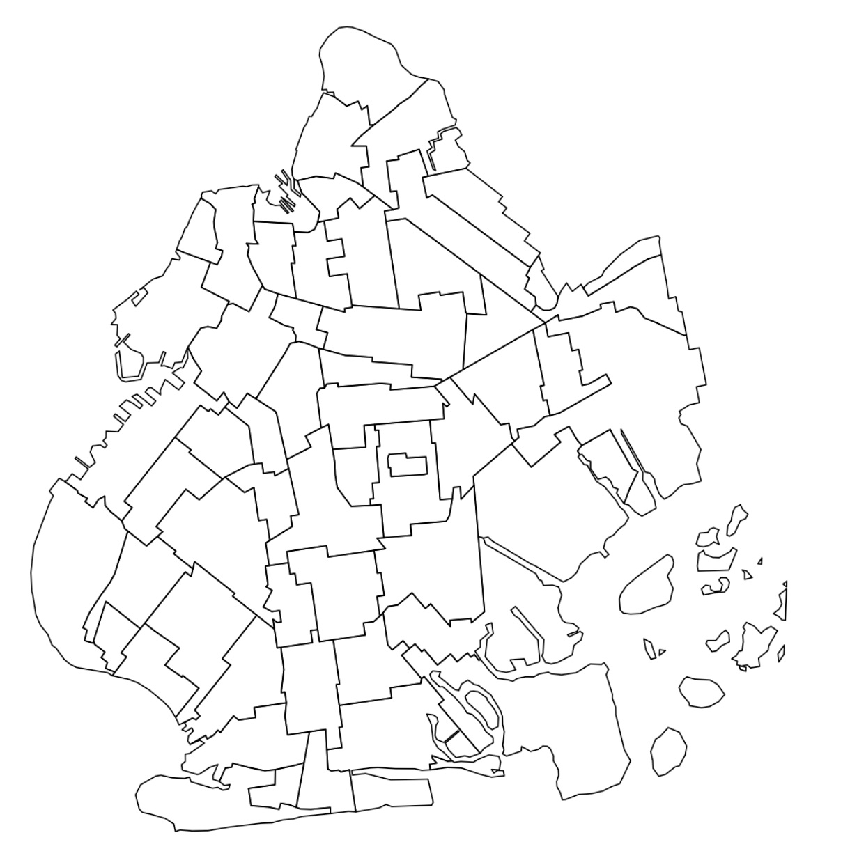 --- # What about `group_by()`? 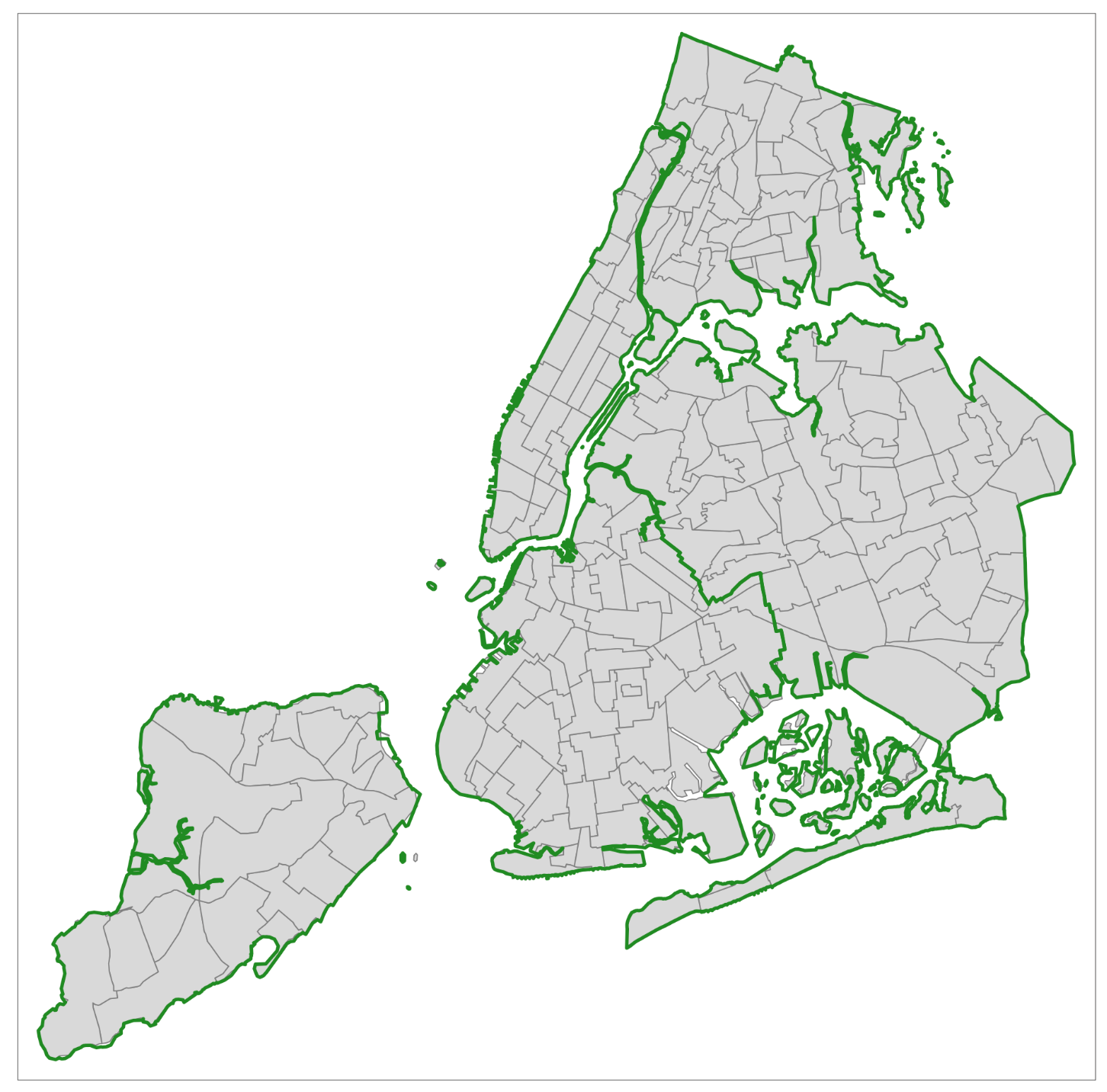 --- # With `group_by()` it groups features into one -- ```r res <- neighborhoods %>% group_by(boro_name) %>% summarize(tot_area = sum(shape_area)) ``` --- # Result of `group_by()` ```r tm_shape(res) + tm_polygons("tot_area") ``` 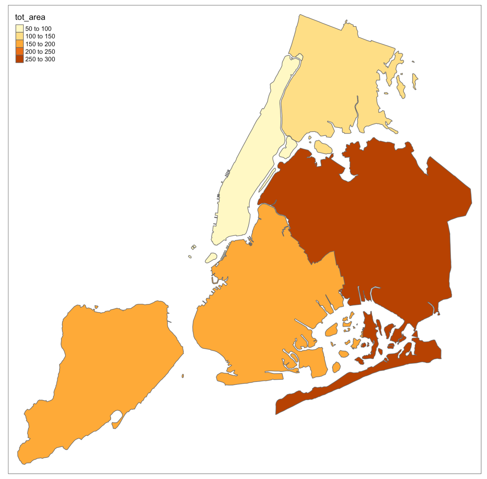 --- # How many columns would you expect in the output here? ```r neighborhoods %>% select(ntacode, ntaname) ``` --- # The geometry is sticky! ```r neighborhoods %>% select(ntacode, ntaname) %>% glimpse() ``` ``` ## Observations: 195 ## Variables: 3 ## $ ntacode <chr> "BK88", "QN51", "QN27", "QN07", "MN0… ## $ ntaname <chr> "Borough Park", "Murray Hill", "East… ## $ geom <MULTIPOLYGON [US_survey_foot]> MULTIPOLYG… ``` --- # Use `st_drop_geometry()` to drop geometry ```r select(neighborhoods, ntacode, ntaname) %>% * st_drop_geometry() %>% glimpse() ``` ``` ## Observations: 195 ## Variables: 2 ## $ ntacode <chr> "BK88", "QN51", "QN27", "QN07", "MN0… ## $ ntaname <chr> "Borough Park", "Murray Hill", "East… ``` --- # This is important, particularly, when joining tables -- ```r glimpse(neighborhoods[,4:7]) ``` ``` ## Observations: 195 ## Variables: 5 ## $ ntaname <chr> "Borough Park", "Murray Hill", "E… ## $ shape_leng <dbl> 11.962555, 10.139753, 6.040134, 6… ## $ boro_name <chr> "Brooklyn", "Queens", "Queens", "… ## $ boro_code <chr> "3", "4", "4", "4", "1", "4", "3"… ## $ geom <MULTIPOLYGON [US_survey_foot]> MULTIPO… ``` -- ```r glimpse(boroughs) ``` ``` ## Observations: 5 ## Variables: 4 ## $ BoroCode <int> 1, 2, 5, 3, 4 ## $ BoroName <chr> "Manhattan", "The Bronx", "Staten… ## $ AreaSqMile <dbl> 22.78279, 42.41274, 58.49555, 71.… ## $ geom <MULTIPOLYGON [°]> MULTIPOLYGON (((-73.… ``` --- # You can't do a tabular join of two {sf} objects -- ```r # Error, two sf objects inner_join(neighborhoods, boroughs, by = c("boro_name" = "BoroName")) ``` ``` ## Error: y should be a data.frame; for spatial joins, use st_join ``` --- # To do the tabular join, drop the geometry from the second object -- ```r boroughs_df <- boroughs %>% st_drop_geometry() ``` -- ```r inner_join(neighborhoods, boroughs_df, by = c("boro_name" = "BoroName")) %>% glimpse() ``` ``` ## Observations: 157 ## Variables: 10 ## $ ntacode <chr> "BK88", "QN51", "QN27", "QN07", … ## $ shape_area <dbl> 5.0172283, 4.8763184, 1.8326831,… ## $ county_fips <chr> "047", "081", "081", "081", "061… ## $ ntaname <chr> "Borough Park", "Murray Hill", "… ## $ shape_leng <dbl> 11.962555, 10.139753, 6.040134, … ## $ boro_name <chr> "Brooklyn", "Queens", "Queens", … ## $ boro_code <chr> "3", "4", "4", "4", "1", "4", "3… ## $ geom <MULTIPOLYGON [US_survey_foot]> MULTIP… ## $ BoroCode <int> 3, 4, 4, 4, 1, 4, 3, 3, 4, 3, 4,… ## $ AreaSqMile <dbl> 71.45976, 109.67223, 109.67223, … ``` --- # Note there is also something called a "spatial join" We will discuss this in section 7 --- background-image: url("images/background-old.jpg") background-size: cover class: center, middle, separator-slide # Getting information about your vector layers --- # Get the coordinate system with `st_crs()` -- ```r st_crs(boroughs) ``` ``` ## Coordinate Reference System: ## EPSG: 4326 ## proj4string: "+proj=longlat +datum=WGS84 +no_defs" ``` --- # Get the bounding box with `st_bbox()` -- ```r boroughs %>% st_bbox() ``` ``` ## xmin ymin xmax ymax ## -74.25589 40.49593 -73.70001 40.91577 ``` --  .footnote[Note that to convert the bbox to a polygon, use `st_as_sfc(st_bbox(obj))`] --- # Get coordinates with `st_coordinates()` Returns all the coordinates that make up your geometry -- ```r schools %>% st_coordinates() %>% head() ``` ``` ## X Y ## 1 980985.1 175780.8 ## 2 988205.1 158329.6 ## 3 992317.3 149703.0 ## 4 986541.2 156991.8 ## 5 976215.3 170325.0 ## 6 983246.6 169950.6 ``` --- # Get the area ```r boroughs %>% st_area() ``` ``` ## Units: [m^2] ## [1] 59007869 109850024 151501538 185080101 284051758 ``` --- # Get the length ```r boroughs %>% st_length() ``` ``` ## Units: [m] ## [1] 103552.31 121146.84 97139.49 175745.68 236701.88 ``` --- # Do you notice something unusual about area and length? -- ```r boroughs %>% st_area() ``` ``` ## Units: [m^2] ## [1] 59007869 109850024 151501538 185080101 284051758 ``` ```r boroughs %>% st_length() ``` ``` ## Units: [m] ## [1] 103552.31 121146.84 97139.49 175745.68 236701.88 ``` --- # Results of calculations like these are class `units` --  --- # Easy to convert between units -- ```r vals <- st_area(boroughs) vals ``` ``` ## Units: [m^2] ## [1] 59007869 109850024 151501538 185080101 284051758 ``` -- ```r units::set_units(vals, km^2) ``` ``` ## Units: [km^2] ## [1] 59.00787 109.85002 151.50154 185.08010 284.05176 ``` .footnote[ [More on units here](https://cran.r-project.org/web/packages/units/vignettes/measurement_units_in_R.html) ] --- # If you add `area` to your data frame... ```r boroughs <- mutate(boroughs, area = st_area(boroughs)) ``` -- ```r boroughs %>% select(area) ``` ``` ## Simple feature collection with 5 features and 1 field ## geometry type: MULTIPOLYGON ## dimension: XY ## bbox: xmin: -74.25589 ymin: 40.49593 xmax: -73.70001 ymax: 40.91577 ## epsg (SRID): 4326 ## proj4string: +proj=longlat +datum=WGS84 +no_defs ## # A tibble: 5 x 2 ## area geom ## * [m^2] <MULTIPOLYGON [°]> ## 1 59007869 (((-73.91839 40.86014, -73.9184 40.8601, -73.91839 40.86008, -… ## 2 109850024 (((-73.78756 40.87256, -73.78723 40.87237, -73.78635 40.87281,… ## 3 151501538 (((-74.05675 40.6081, -74.05664 40.608, -74.05559 40.60663, -7… ## 4 185080101 (((-73.98569 40.5813, -73.98368 40.58303, -73.98253 40.58229, … ## 5 284051758 (((-73.70089 40.74706, -73.70078 40.74504, -73.70058 40.74318,… ``` --- # But units can be a pain at times -- ```r library(ggplot2) # Error, doesn't like units ggplot(boroughs, aes(area)) + geom_histogram() ``` ``` ## Error in Ops.units(x, range[1]): both operands of the expression should be "units" objects ``` <img src="5-vector-data_files/figure-html/unnamed-chunk-61-1.png" style="display: block; margin: auto;" /> --- # Sometimes I prefer to drop the units -- ```r boroughs <- boroughs %>% mutate(area = units::drop_units(area)) ``` -- ```r ggplot(boroughs, aes(area)) + geom_histogram() ``` <img src="5-vector-data_files/figure-html/unnamed-chunk-63-1.svg" style="display: block; margin: auto;" /> --- background-image: url("images/background-old.jpg") background-size: cover class: center, middle, separator-slide # Converting to `sp` and between geometry types --- # Convert to an `sp` object --- # For a limited number of packages you need this old type --- # Convert with `as()` -- ```r boroughs_sp <- as(boroughs, "Spatial") boroughs_sp ``` ``` ## class : SpatialPolygonsDataFrame ## features : 5 ## extent : -74.25589, -73.70001, 40.49593, 40.91577 (xmin, xmax, ymin, ymax) ## crs : +proj=longlat +datum=WGS84 +no_defs +ellps=WGS84 +towgs84=0,0,0 ## variables : 4 ## names : BoroCode, BoroName, AreaSqMile, area ## min values : 1, Brooklyn, 22.782792843, 59007869.4207004 ## max values : 5, The Bronx, 109.672225243, 284051758.495162 ``` --- # Convert back to `sf` with `as()` -- ```r boroughs_sf <- as(boroughs, "sf") boroughs_sf ``` ``` ## Simple feature collection with 5 features and 4 fields ## geometry type: MULTIPOLYGON ## dimension: XY ## bbox: xmin: -74.25589 ymin: 40.49593 xmax: -73.70001 ymax: 40.91577 ## epsg (SRID): 4326 ## proj4string: +proj=longlat +datum=WGS84 +no_defs ## # A tibble: 5 x 5 ## BoroCode BoroName AreaSqMile geom area ## * <int> <chr> <dbl> <MULTIPOLYGON [°]> <dbl> ## 1 1 Manhattan 22.8 (((-73.91839 40.86014, -73.9184 40… 5.90e7 ## 2 2 The Bronx 42.4 (((-73.78756 40.87256, -73.78723 4… 1.10e8 ## 3 5 Staten Is… 58.5 (((-74.05675 40.6081, -74.05664 40… 1.52e8 ## 4 3 Brooklyn 71.5 (((-73.98569 40.5813, -73.98368 40… 1.85e8 ## 5 4 Queens 110. (((-73.70089 40.74706, -73.70078 4… 2.84e8 ``` --- # Converting between geometry with `st_cast()` --- # For example, change Manhattan from a polygon to points ```r manhattan <- filter(boroughs, BoroName == "Manhattan") ``` -- ```r manhattan_pt <- st_cast(manhattan, 'POINT') ``` --- # Plot Manhattan as points Do you remember what function we use to extract the geometry? -- ```r plot(st_geometry(manhattan_pt), cex = 0.5, col = "cadetblue") ``` <img src="5-vector-data_files/figure-html/unnamed-chunk-69-1.svg" width="65%" style="display: block; margin: auto;" /> --- class: center, middle, doExercise # open_exercise(5) and finish the activities