class: title-slide background-size: cover <h1 class="center middle">Visualizing Spatial Data</h1> <h3 class="center middle">(static and interactive maps)</h3> <div class="logo"></div> <div class="databird"></div> --- # R has great map-making functionality! --- # This map was created in R  .footnote[ [Source: Timo Grossenbacher](https://timogrossenbacher.ch/2019/04/bivariate-maps-with-ggplot2-and-sf/) ] --- # This map was created in R 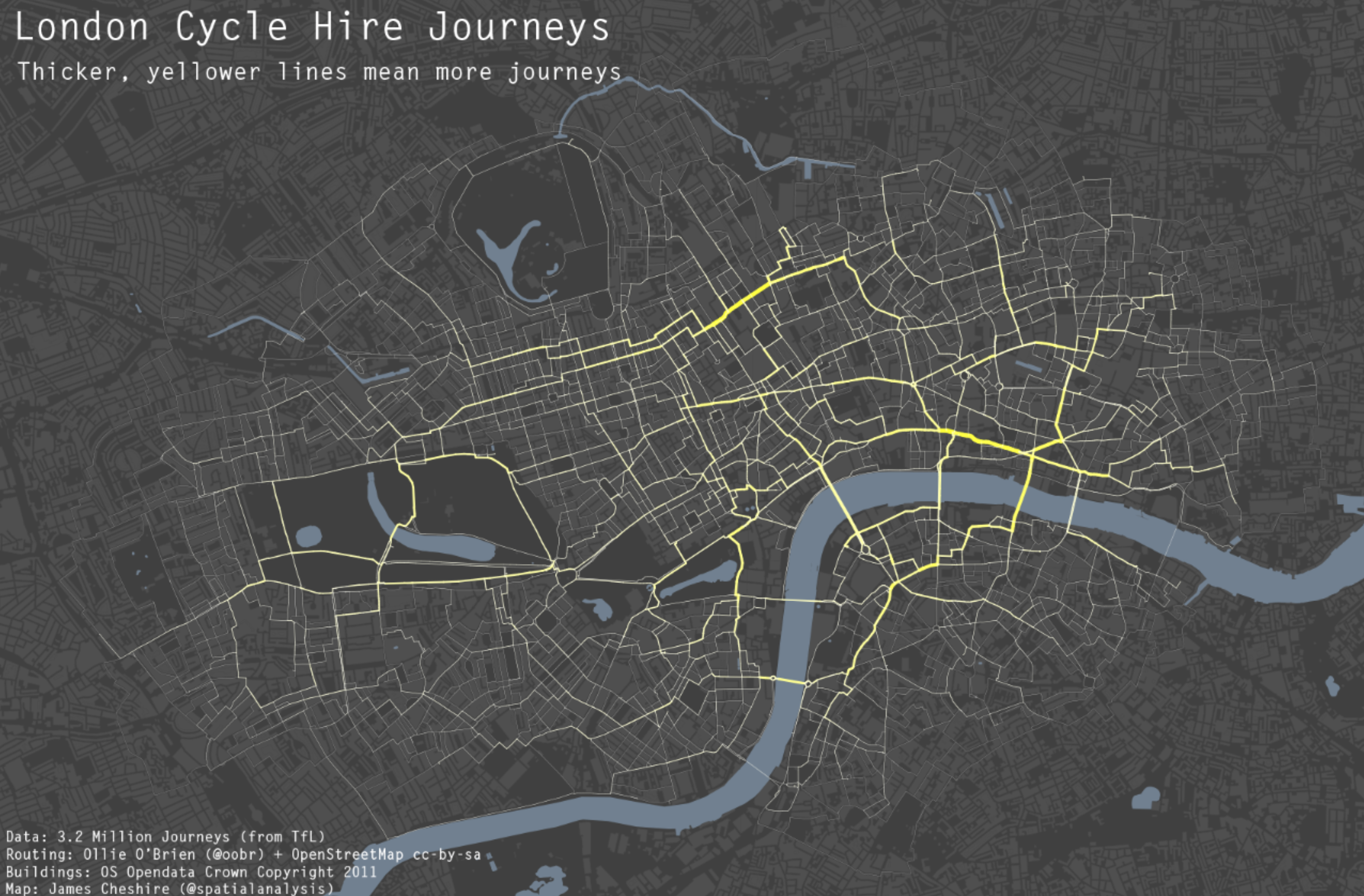 .footnote[ [Source: spatial.ly](http://spatial.ly/2012/02/great-maps-ggplot2/) ] --- # This map was created in R  .footnote[ [Source: rayshader](https://github.com/tylermorganwall/rayshader) ] --- # What packages should you use? --- # There are dozens of mapping-related packages in R -- * But only a few are all-purpose --- # All-purpose static mapping * The `plot()` function * {tmap} * {ggplot2} (we won't cover {ggplot2}) --- # All-purpose interactive mapping * {tmap} * {mapview} * {leaflet} (we won't cover {leaflet}) --- exclude:true # Color palettes * [{viridis}](https://cran.r-project.org/web/packages/viridis/vignettes/intro-to-viridis.html) * [{RColorBrewer}](https://cran.r-project.org/web/packages/RColorBrewer/index.html) * [{swatches}](https://github.com/hrbrmstr/swatches) * [{ggthemes}](https://cran.r-project.org/web/packages/ggthemes/index.html) --- # A lot of great packages for niche mapping needs * {rayshader} * {geogrid} * {globe} * {linemap} * {cartogram} * {cartography} * {mapedit} * {rasterVis} --- background-image: url("images/background-old.jpg") background-size: cover class: center, middle, separator-slide # Static mapping --- # Take home messages -- * I use `plot()` for a quick look at data -- * I use {tmap} for everything else -- * {tmap} has an insane amount of customization allowed, we will only touch the surface --- # Why not `ggplot2`? -- * I love `ggplot2` and use it every day -- * But I find making maps significantly easier in `tmap` * Can do almost anything in `tmap` * Easy to include just fill, just borders, etc * Interactive views * etc... --- # But I will show a ggplot-map at the end of this section --- class: center, middle # `plot()` --- # Yes `plot()` is not super exciting  --- # But `plot()` is great for a quick look at your data --- # `plot()` has methods for vector and raster data -- The packages need to be loaded to plot vector and raster data --- # Some setup: load packages No need to type with me, you'll practice in the exercise ```r library(sf) # read vectors library(raster) # read rasters library(tmap) # mapping ``` --- # Some setup: read in NYC data ```r boroughs <- read_sf("boroughs.gpkg") schools <- read_sf("schools.shp") canopy <- raster("canopy.grd") ``` --- # With vectors the default is to plot the attributes ```r plot(boroughs) ``` -- 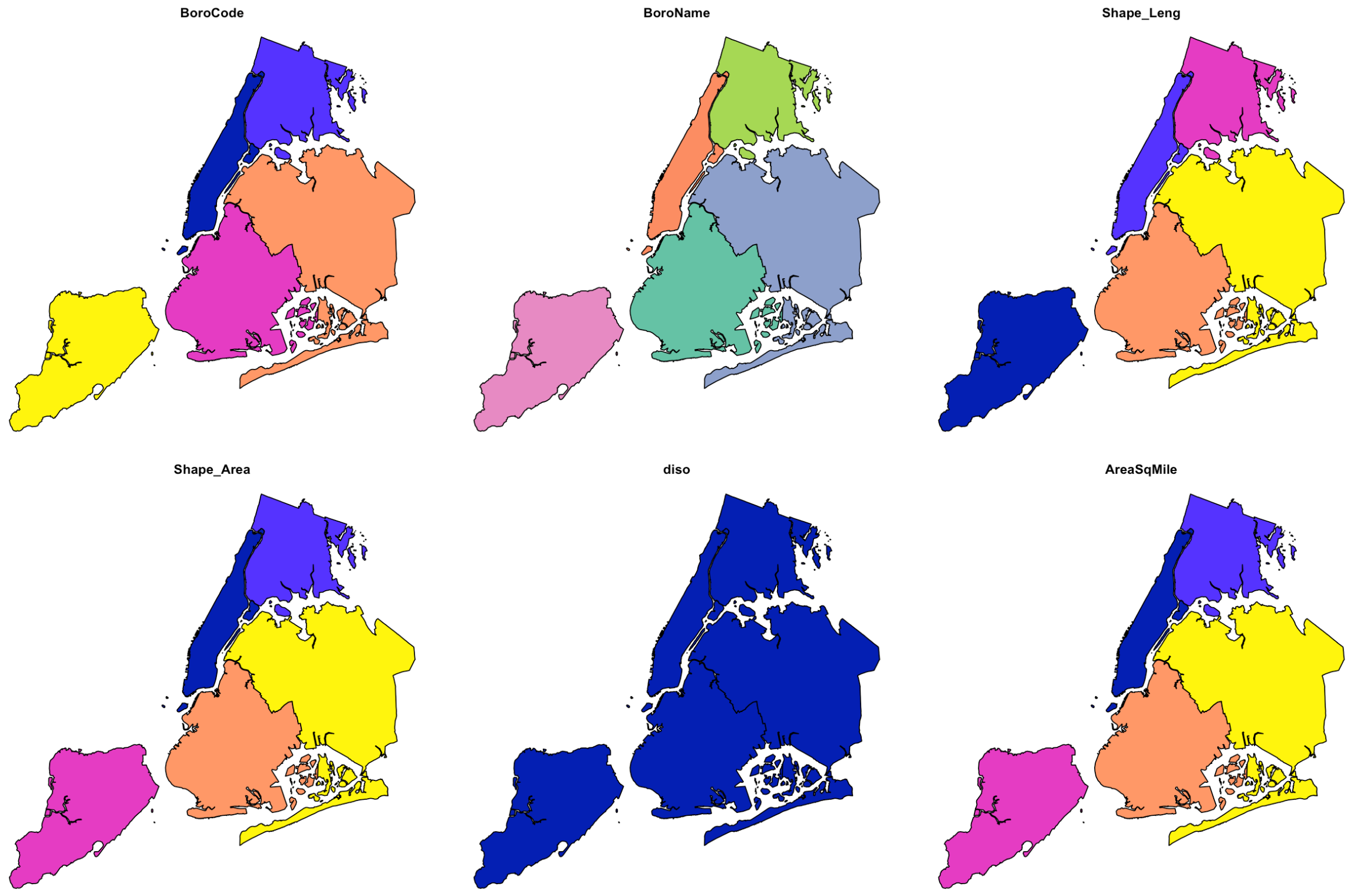 --- # I don't really like this default  --- # You can plot a single attribute -- ```r plot(boroughs['Shape_Area'], main = "Area", pal = rev(heat.colors(5))) ``` 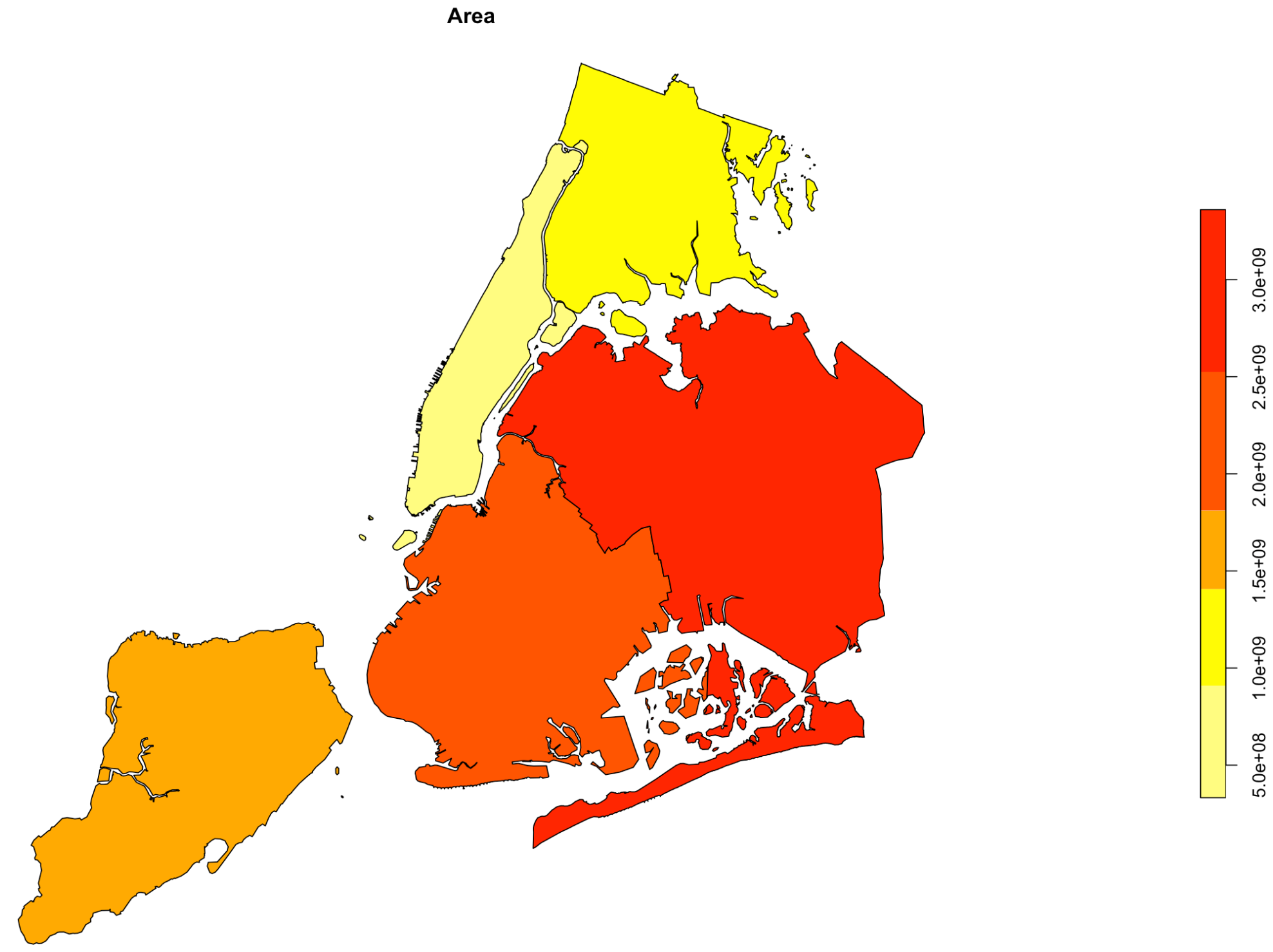 --- # For a quick look at vectors, I often just want the geometry -- * You can extract just the geometry with `st_geometry()` -- * Then call `plot()` on the output --- # `st_geometry()` and then plot ```r st_geometry(boroughs) %>% plot() ```  --- # Or wrap the two functions ```r plot(st_geometry(boroughs)) ```  --- # Try to memorize this concept/code ```r st_geometry(boroughs) %>% plot() ``` ```r plot(st_geometry(boroughs)) ``` --- # To combine layers with `plot()` use `add = TRUE` ```r plot(st_geometry(boroughs)) plot(st_geometry(schools), add = TRUE, pch = 16, col = "red", cex = 0.5) ```  --- # Careful with `add = TRUE`, only works with `st_geometry()` -- ```r # This won't work! plot(boroughs) plot(schools, add = TRUE) ``` <img src="3-mapping_files/figure-html/unnamed-chunk-10-1.png" style="display: block; margin: auto;" /> --- # Easy to use `plot()` with rasters ```r plot(canopy) # a single band raster ```  --- # If your raster has multiple layers (like an image) ... `plot()` maps each layer separately ```r plot(manhattan) ``` --  --- # If your raster has a red, green and blue layer (like an image) You can plot them together... -- ```r plotRGB(manhattan) ``` 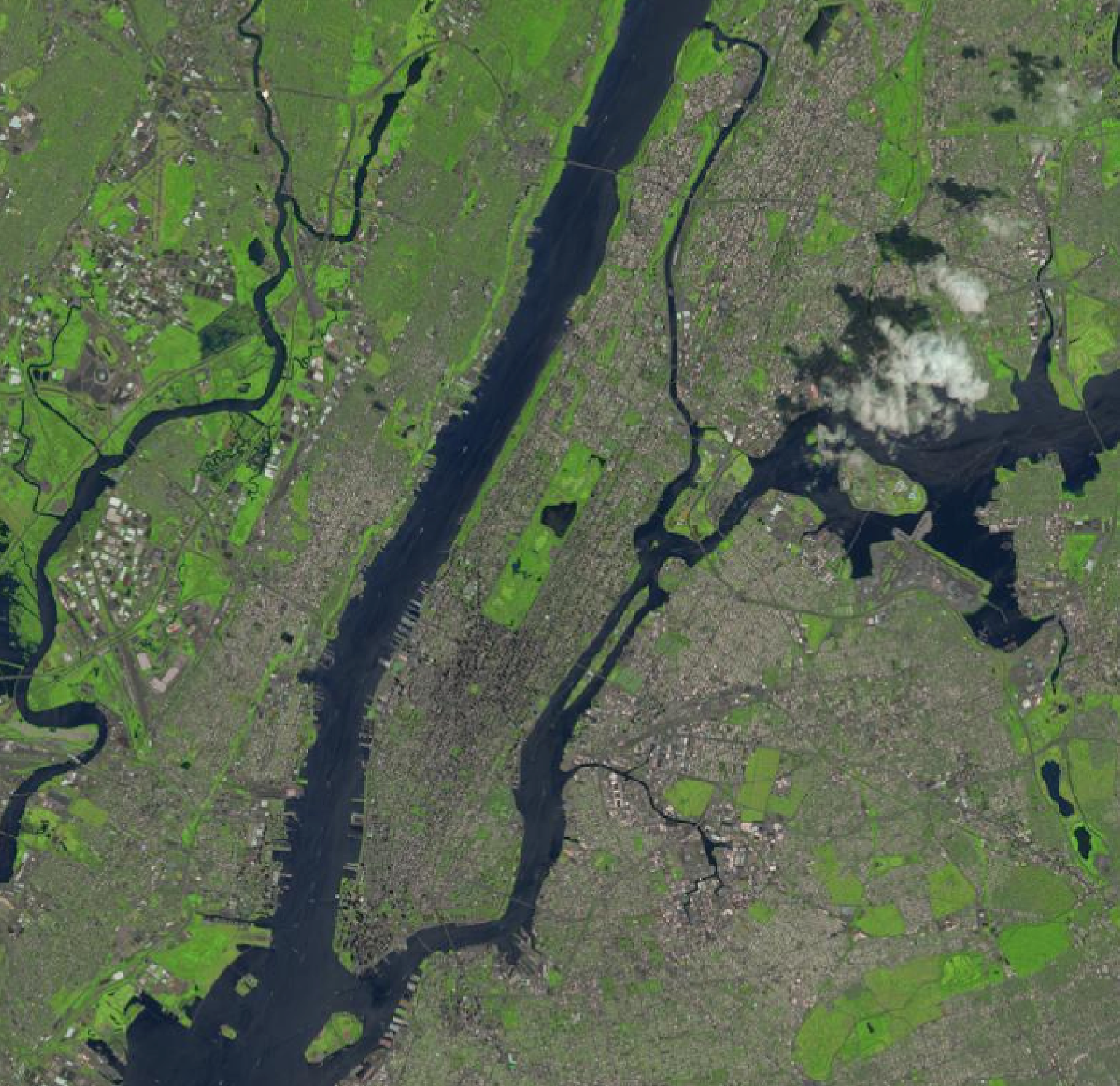 --- # Combine rasters and vectors with `plot()` -- ```r plot(canopy) plot(st_geometry(schools), add = T, pch = 16, col = "red", cex = 0.5) ``` 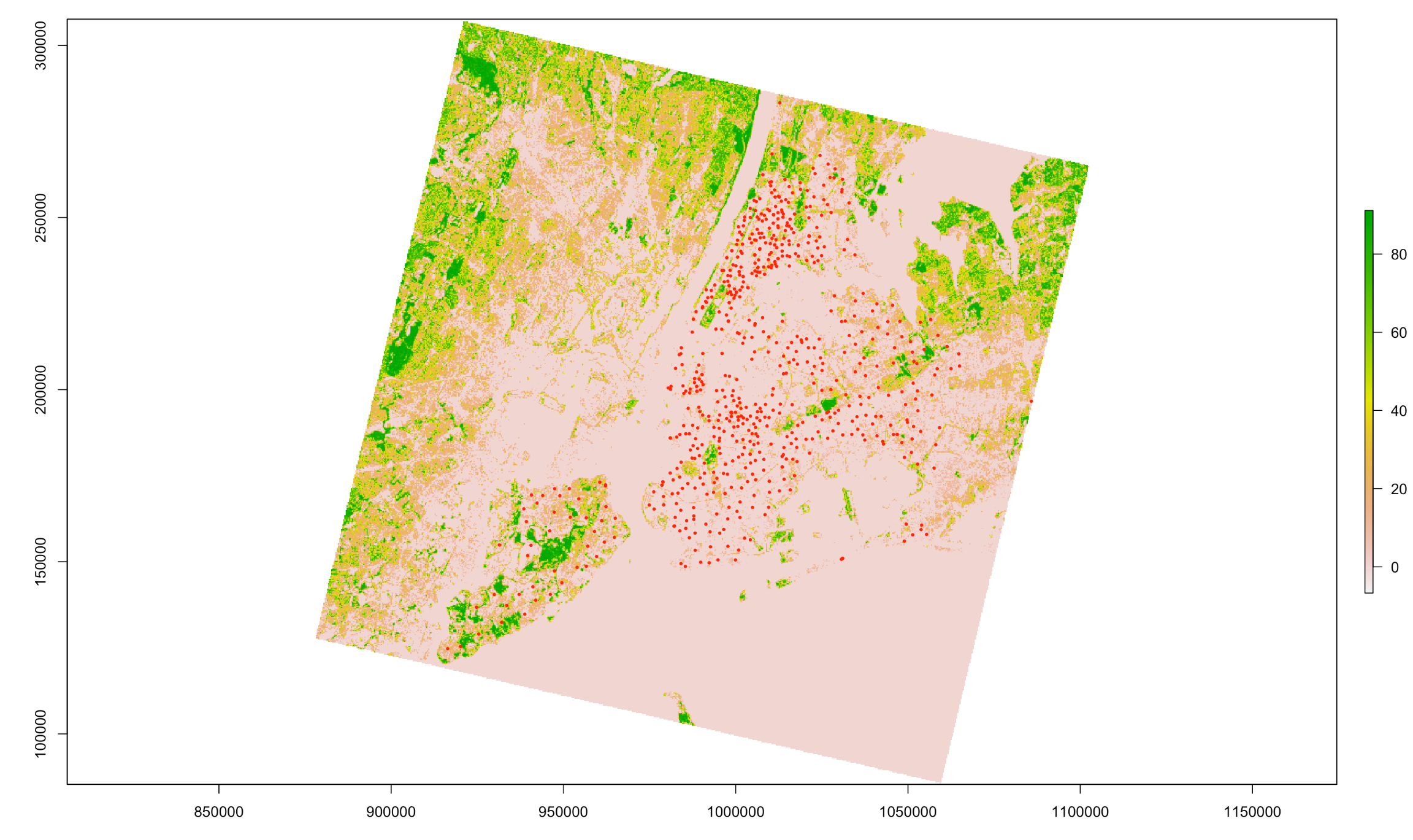 --- # For more sophisticated and fun static maps I use {tmap} --- class: center, middle # {tmap} --- # So much control with {tmap}! -- ```r tm_text(text, size = 1, col = NA, root = 3, clustering = FALSE, size.lim = NA, sizes.legend = NULL, sizes.legend.labels = NULL, sizes.legend.text = "Abc", n = 5, style = ifelse(is.null(breaks), "pretty", "fixed"), breaks = NULL, interval.closure = "left", palette = NULL, labels = NULL, labels.text = NA, midpoint = NULL, stretch.palette = TRUE, contrast = NA, colorNA = NA, textNA = "Missing", showNA = NA, colorNULL = NA, fontface = NA, fontfamily = NA, alpha = NA, case = NA, shadow = FALSE, bg.color = NA, bg.alpha = NA, size.lowerbound = 0.4, print.tiny = FALSE, scale = 1, auto.placement = FALSE, remove.overlap = FALSE, along.lines = FALSE, overwrite.lines = FALSE, just = "center", xmod = 0, ymod = 0, title.size = NA, title.col = NA, legend.size.show = TRUE, legend.col.show = TRUE, legend.format = list(), legend.size.is.portrait = FALSE, legend.col.is.portrait = TRUE, legend.size.reverse = FALSE, legend.col.reverse = FALSE, legend.hist = FALSE, legend.hist.title = NA, legend.size.z = NA, legend.col.z = NA, legend.hist.z = NA, group = NA, auto.palette.mapping = NULL, max.categories = NULL) ``` --- # {tmap} syntax is similar to {ggplot2} ```r # data set up layer tm_shape(boroughs) + tm_polygons() ``` -- 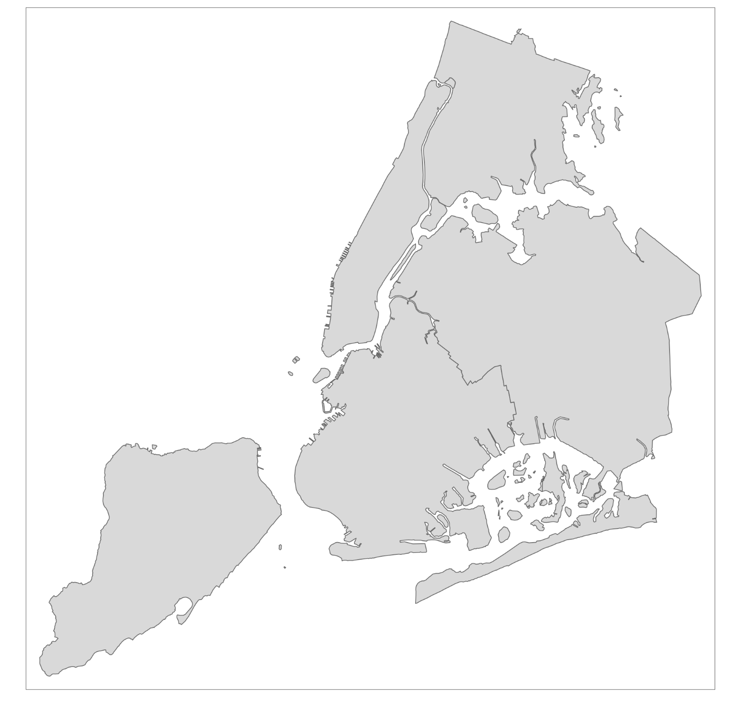 --- # A short-cut `qtm()` Instead of `plot()` I often use this ```r qtm(boroughs) ```  --- # Add multiple layers based on one input ```r tm_shape(boroughs) + tm_polygons() + tm_dots(size = 2) + tm_text("BoroName", col = "red", size = 1.5) ``` -- 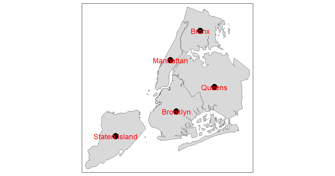 --- # Or multiple different layers using multiple shapes -- ```r tm_shape(boroughs) + tm_borders() + tm_shape(schools) + tm_dots(size = 0.25) ``` 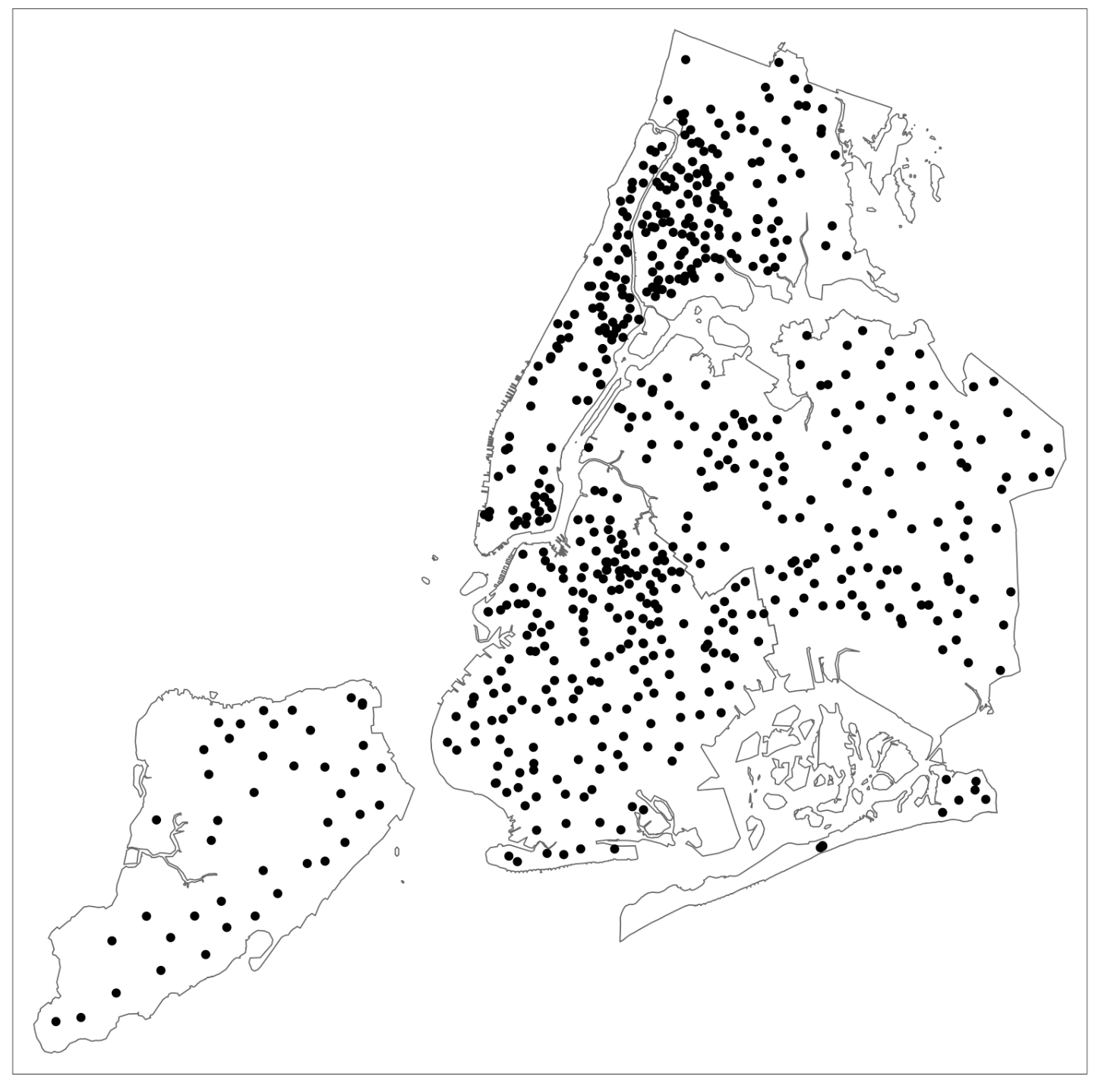 --- # You can also save parts of the map and reuse ```r mymap <- tm_shape(boroughs) + tm_polygons() ``` -- ```r mymap + tm_dots(size = 2) + tm_text("BoroName", col = "red") ```  --- # Choropleth (color-coded map) based on a variable. So easy! ```r tm_shape(boroughs) + tm_polygons("Shape_Area") ``` -- 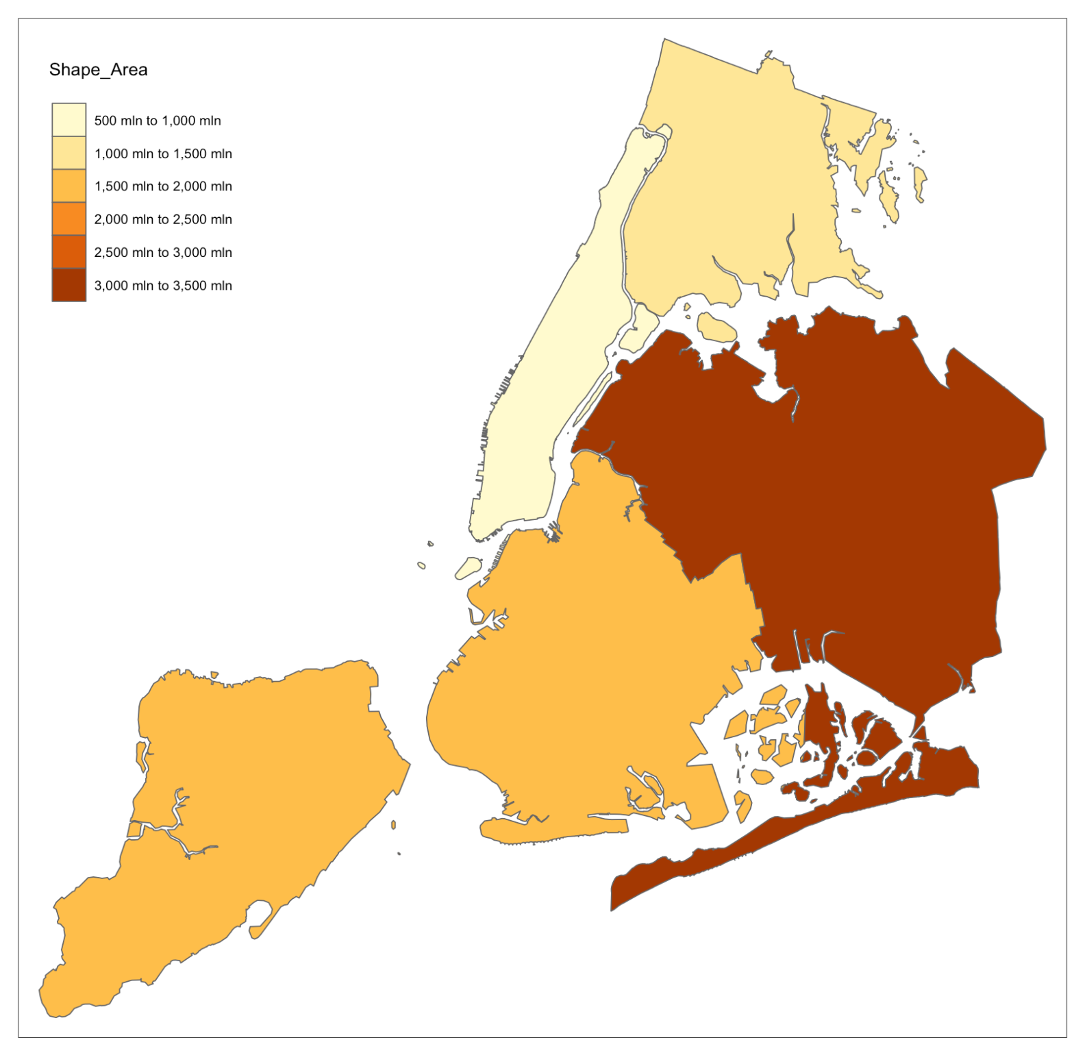 --- # Or show an attribute with `tm_symbols()` ```r tm_shape(boroughs) + tm_borders() + tm_symbols("Shape_Area", scale = 2) ``` 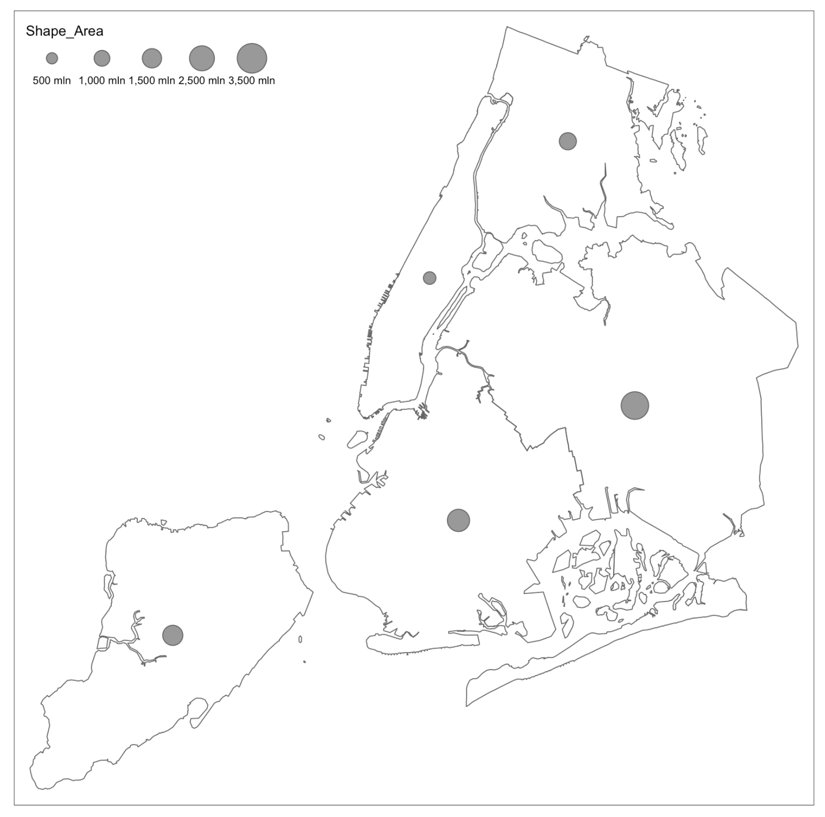 --- # Plot multiple variables at once ```r tm_shape(boroughs) + tm_polygons(c("Shape_Area", "BoroName")) ``` 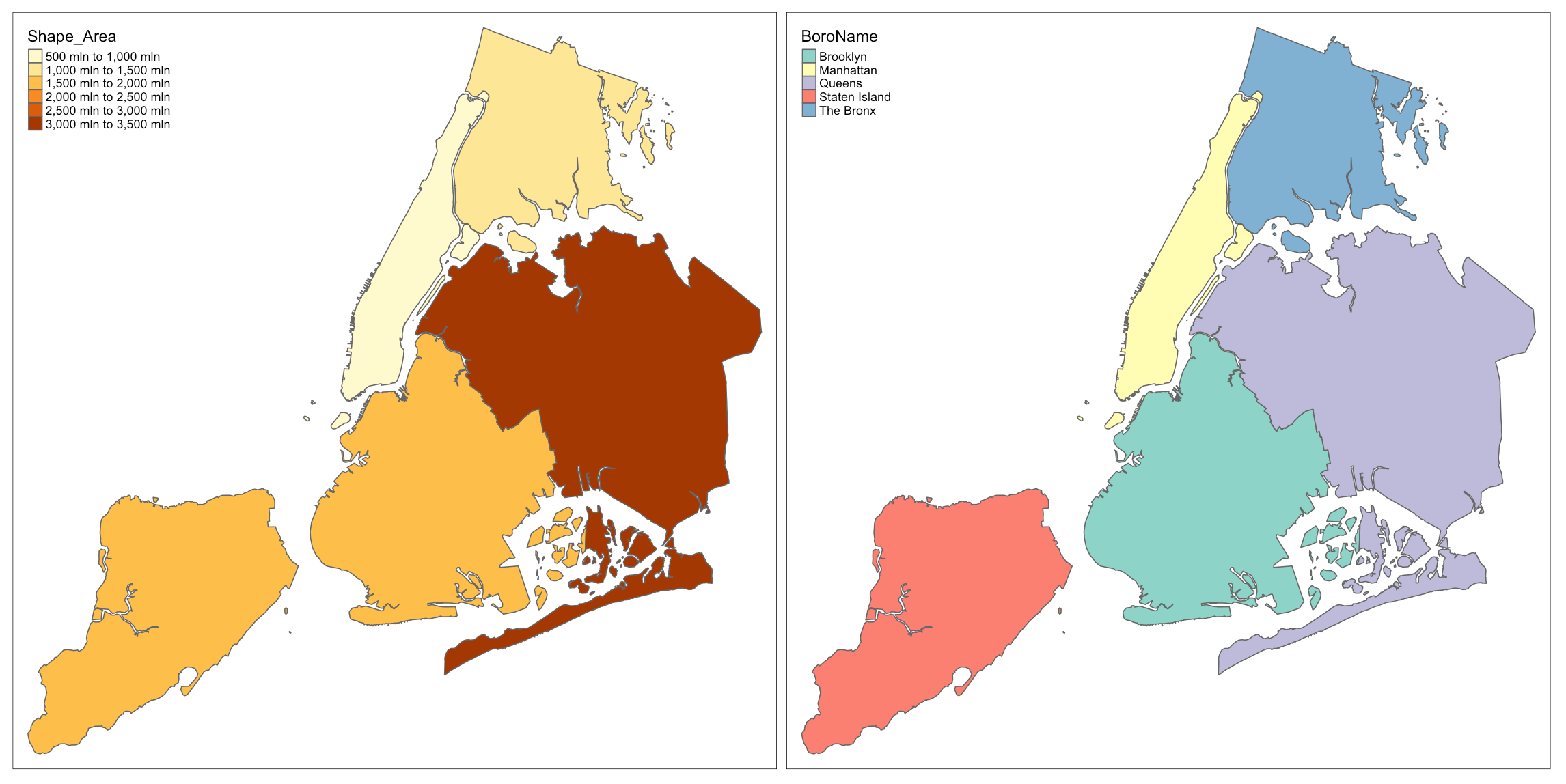 --- # `tm_shape()` can accept vector or raster  --- # Single-band raster with `tm_raster()` ```r tm_shape(canopy) + tm_raster() ``` -- 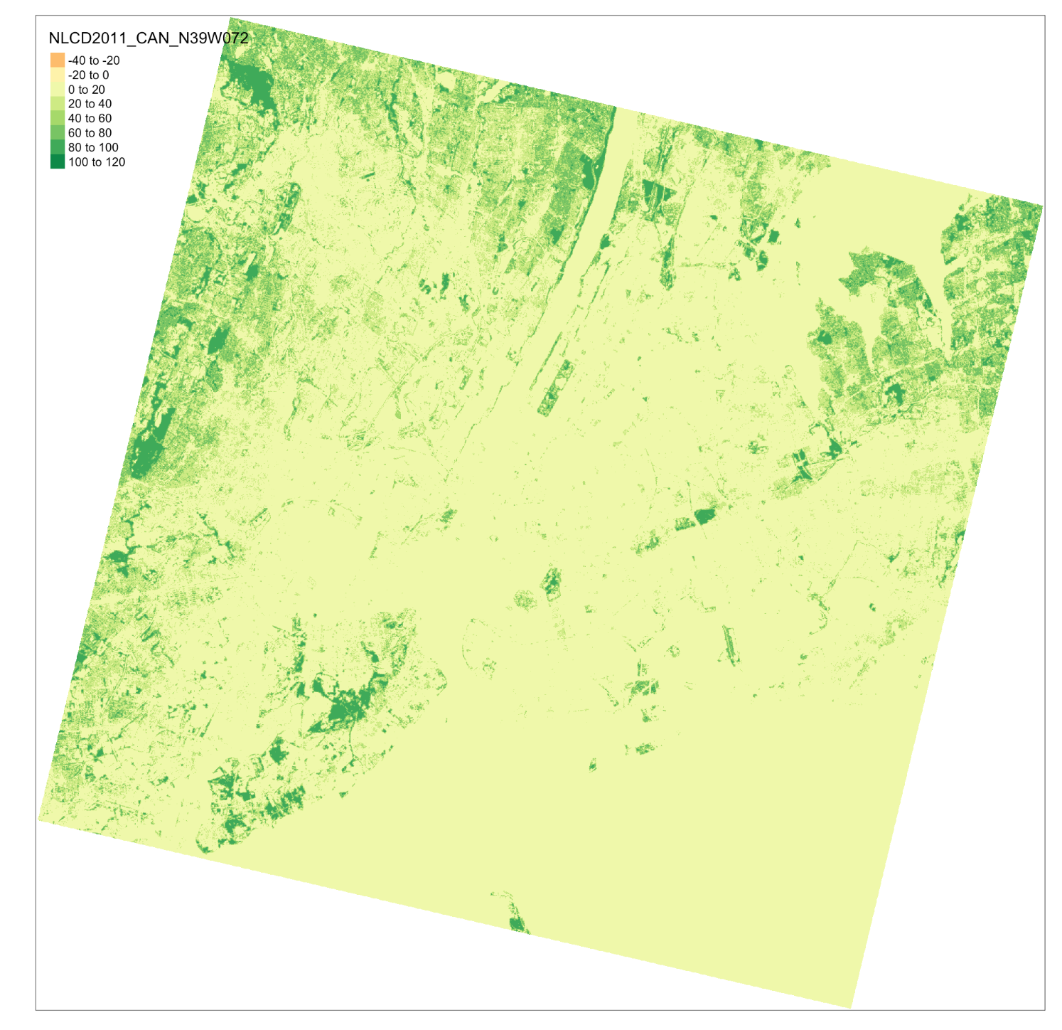 --- # A multi-layer raster with `tm_rgb()` ```r tm_shape(manhattan) + tm_rgb() ``` --  --- # Vector and raster ```r tm_shape(manhattan) + tm_rgb()+ tm_shape(boroughs) + tm_borders(col = "white", lwd = 2) ``` -- 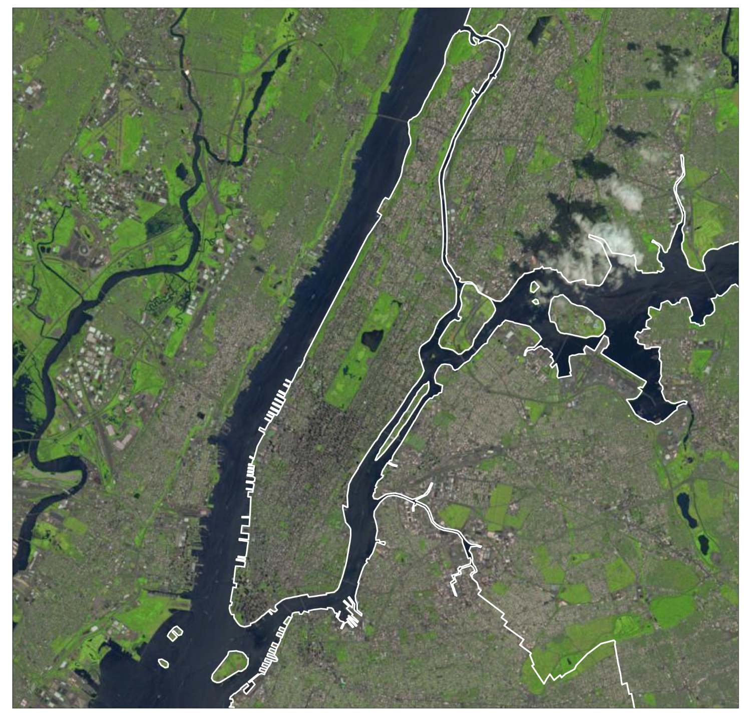 --- # Include a basemap in your map Use a function from the companion package, {tmaptools} -- ```r osmtiles <- tmaptools::read_osm(boroughs, type="stamen-terrain") ``` --- # Include a basemap in your map ```r tm_shape(osmtiles) + tm_raster() + tm_shape(boroughs) + tm_borders(lwd = 2, col = "yellow") ``` 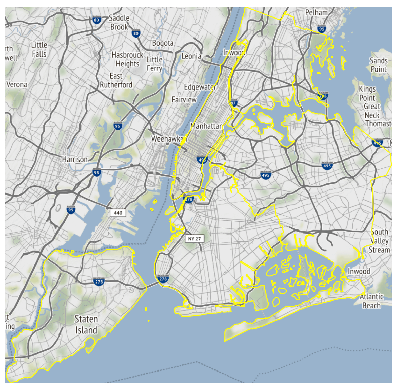 --- # Map extent is driven by the "master" * First shape is master by default -- * in tm_shape() can use `is.master = TRUE` --- # Here is the default (extent based on raster) ```r tm_shape(canopy) + tm_raster(title = "(percent canopy)", alpha = 0.75) + tm_shape(boroughs) + tm_borders(lwd = 2, col = "blue") ``` 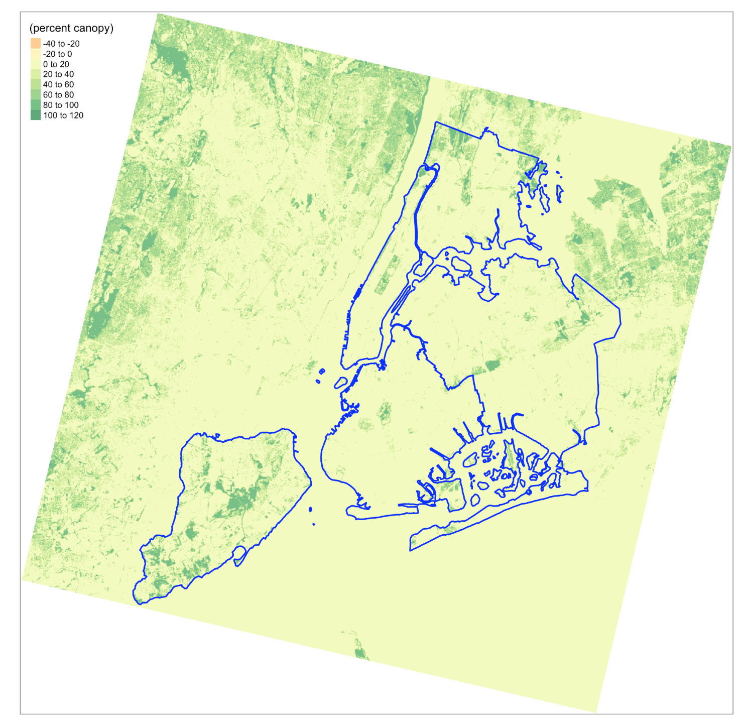 --- # Force the extent to be the polygon borders ```r tm_shape(canopy) + tm_raster(title = "(percent canopy)", alpha = 0.75) + tm_shape(boroughs, is.master = TRUE) + tm_borders(lwd = 2, col = "blue") ``` -- 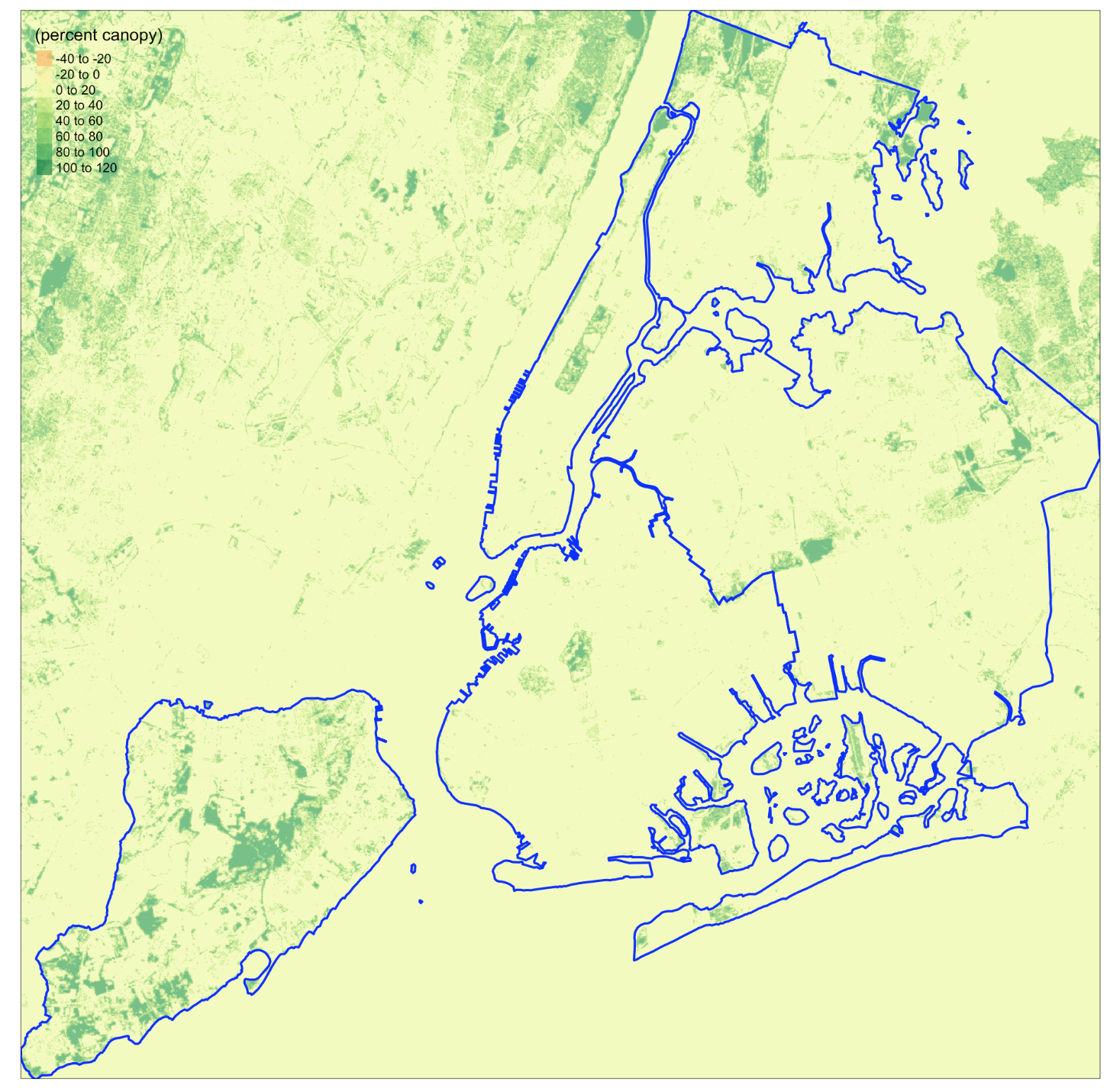 --- # Using color palettes in `tmap` * [`viridis`](https://cran.r-project.org/web/packages/viridis/vignettes/intro-to-viridis.html) * [`RColorBrewer`](http://colorbrewer2.org/#type=sequential&scheme=BuGn&n=3) --- # `palette_explorer()` is great ```r tmaptools::palette_explorer() ``` 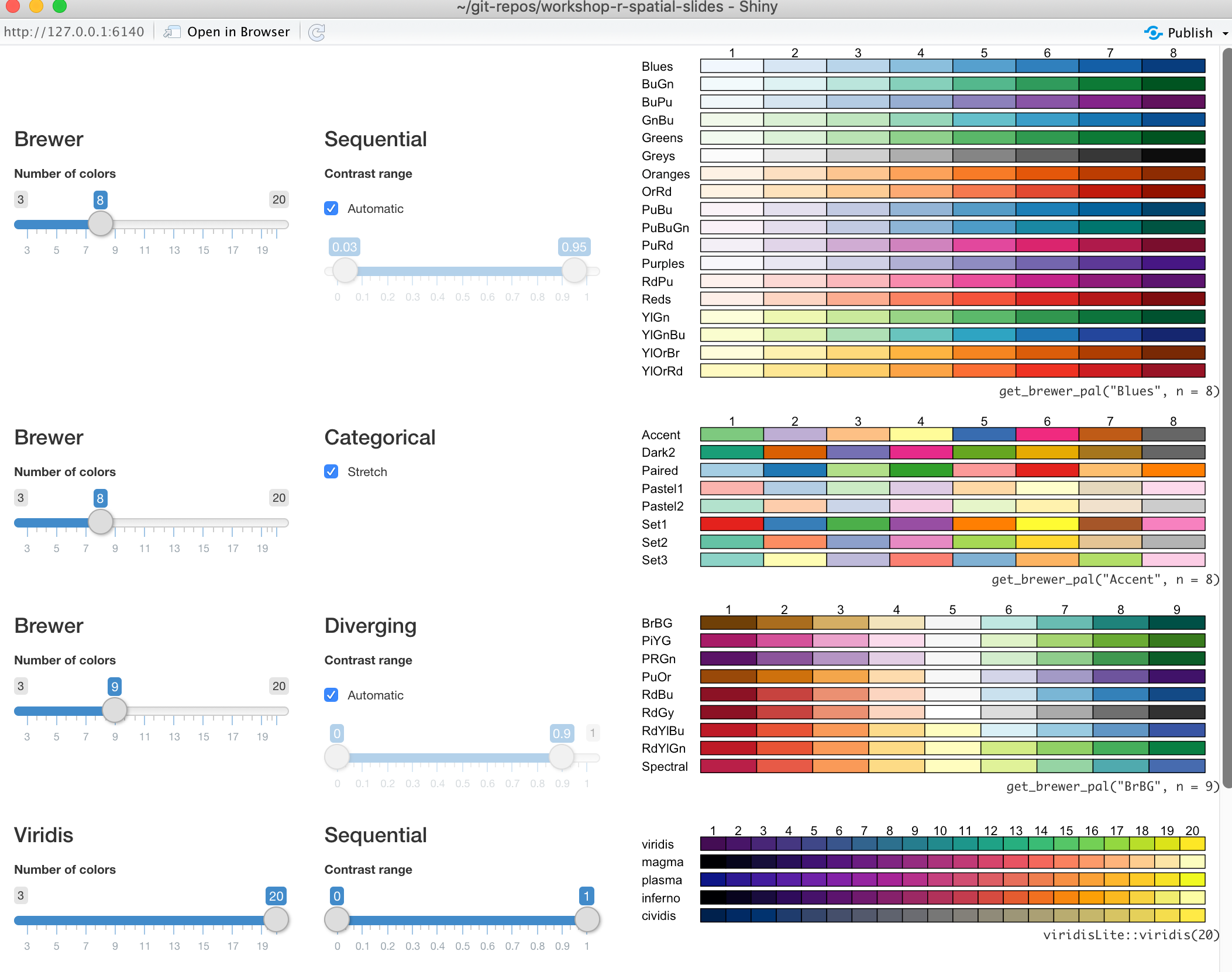 --- # Use a palette with the `pal` argument ```r tm_shape(neighborhoods) + tm_polygons("shape_area", n = 5, pal = "Greens") ``` -- 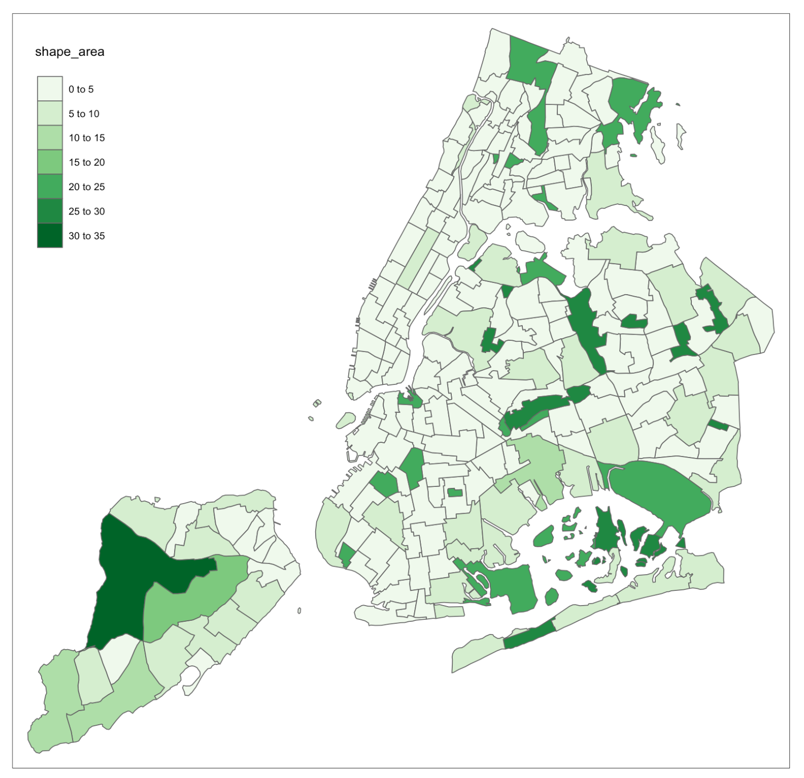 --- # Use `-` to reverse the palette ```r tm_shape(neighborhoods) + tm_polygons("shape_area", n = 5, pal = "-Greens") ``` -- 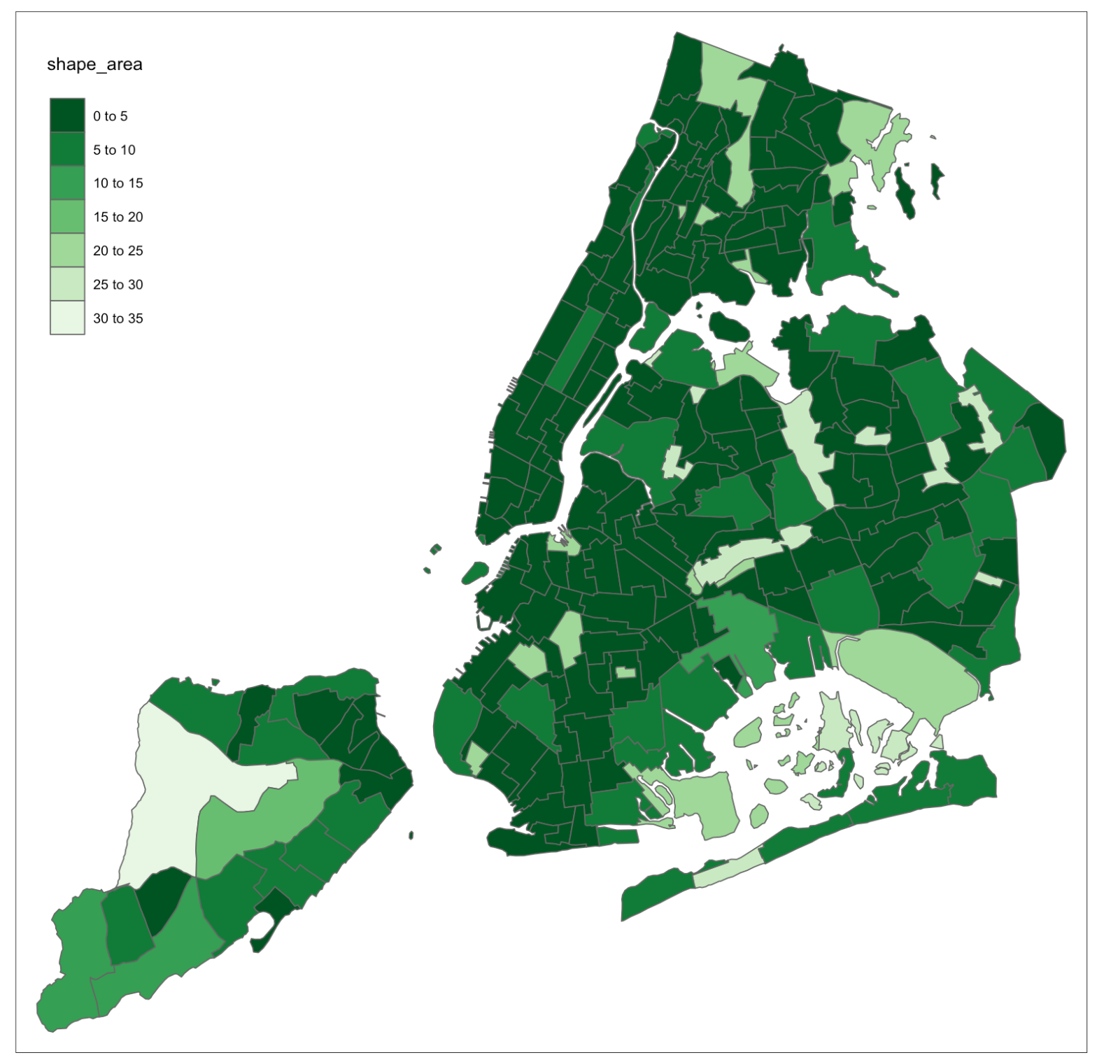 --- # Alter the map layout with `tm_layout()` -- ```r tm_shape(neighborhoods) + tm_polygons("shape_area", n = 5, pal = "Greens") + tm_layout(legend.show = FALSE, frame = FALSE) ``` 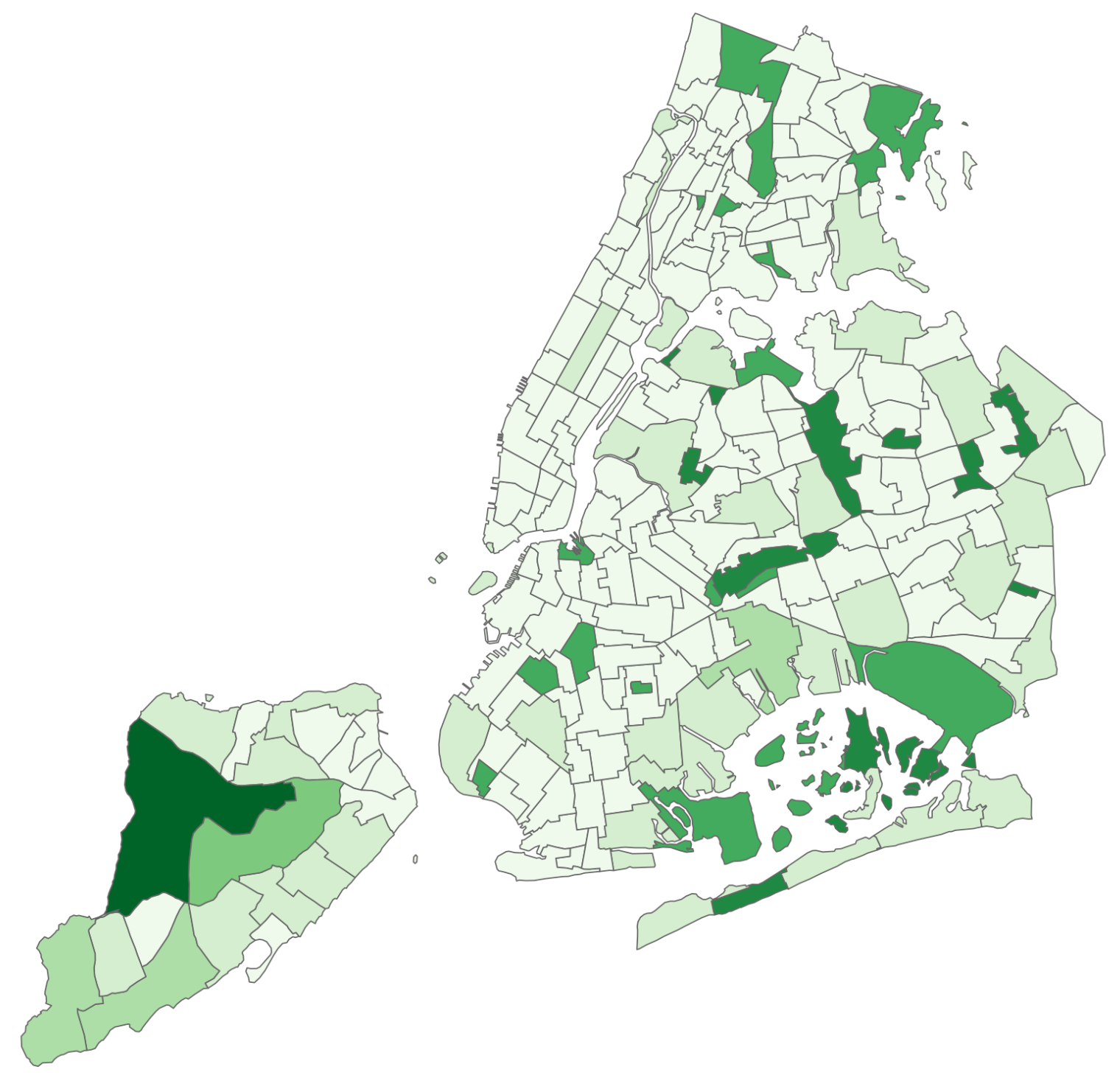 --- # Save your maps with `tmap_save()` -- ```r mymap <- tm_shape(boroughs) + tm_polygons() tmap_save(mymap, "mymap.png") ``` --- # It's easy to include more than one map in an image with `tmap_arrange()` -- ```r # Create three maps m1 <- tm_shape(boroughs) + tm_polygons() m2 <- tm_shape(neighborhoods) + tm_polygons() m3 <- tm_shape(schools) + tm_dots(size = 0.25) ``` --- # Arrange them on one image -- ```r tmap_arrange(m1, m2, m3, nrow = 1) ``` -- <img src="3-mapping_files/figure-html/unnamed-chunk-42-1.svg" style="display: block; margin: auto;" /> --- # So many great other functions to explore * `tmap_save()` * `tm_layout()` * `tm_style()` * `tm_facets()` * `tm_animation()` * `tm_scale_bar()` * `tm_compass()` --- # As promised earlier, three slides on mapping with {ggplot2} --- # {ggplot2} has a special layer for {sf} objects -- * `geom_sf()` --- # With `geom_sf()` no need to specify x and y * Unlike `geom_line()`, `geom_points()` etc --- # To create a choropleth use `aes()` with the fill argument -- ```r library(ggplot2) ggplot() + geom_sf(data = boroughs, aes(fill = BoroCode)) + geom_sf(data = schools, color = "purple") ``` <img src="3-mapping_files/figure-html/unnamed-chunk-43-1.svg" style="display: block; margin: auto;" /> --- # You can also make nice maps with {ggplot2}  .footnote[ [Source: Timo Grossenbacher](https://timogrossenbacher.ch/2019/04/bivariate-maps-with-ggplot2-and-sf/) ] --- # Keep in mind, there are other packages worth exploring --- # Quick example of geogrid 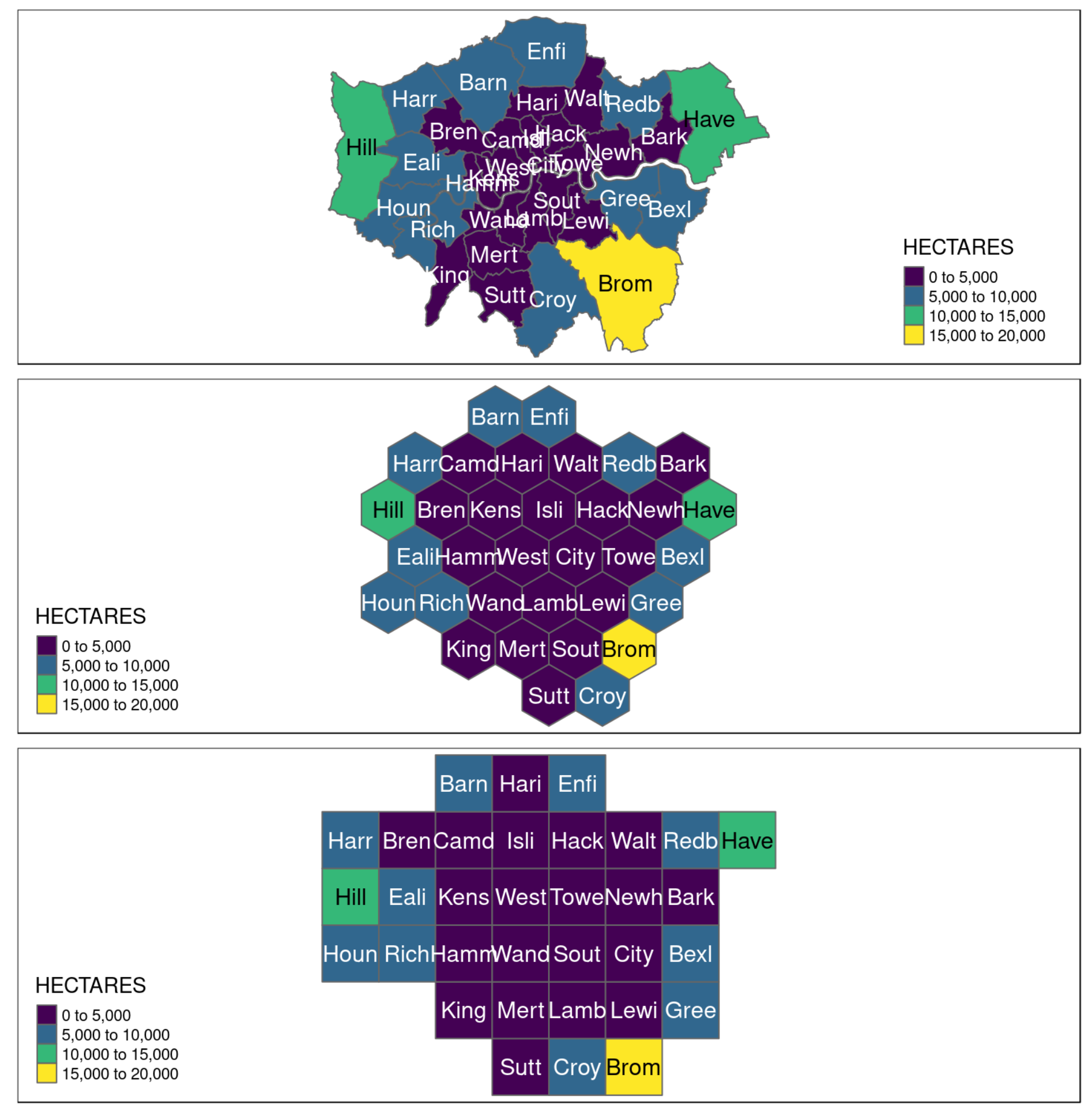 .footnote[ https://github.com/jbaileyh/geogrid ] --- # Hillshading with rayshader  .footnote[ https://github.com/tylermorganwall/rayshader ] --- # Cartographic representations with {cartography} 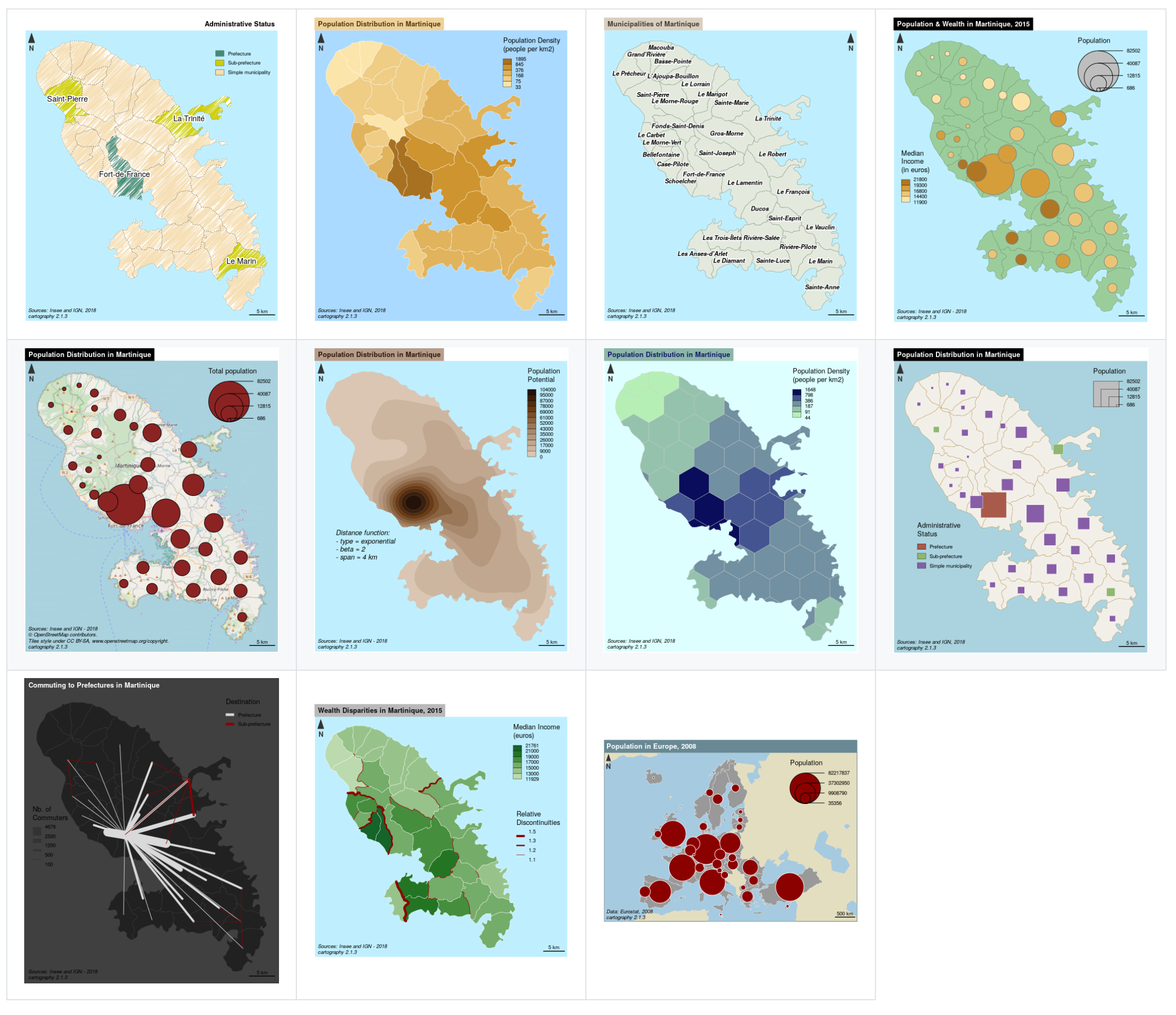 .footnote[ https://github.com/riatelab/cartography ] --- class: center, middle, doExercise # open_exercise(3) and work on activity 1-9 then stop --- background-image: url("images/background-old.jpg") background-size: cover class: center, middle, separator-slide # Interactive maps --- # There are two packages I use for interactive maps * {mapview} (for a quick interactive look) * {tmap} (for a more polished interactive map) --- # Why not RStudio's {leaflet} * Main reason is it requires layers to be unprojected (we will discuss) * There are work-arounds like `leafletCRS()` * But {tmap} and {mapview} do a great job --- # Both {tmap} and {mapview} also use the Leaflet JavaScript API 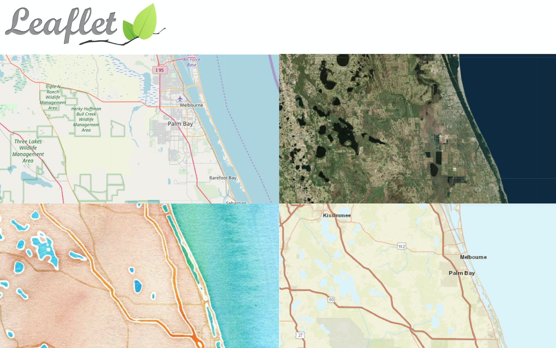 --- # Since we're already talking about {tmap} let's start with {tmap} --- # Remember this static {tmap} from earlier? 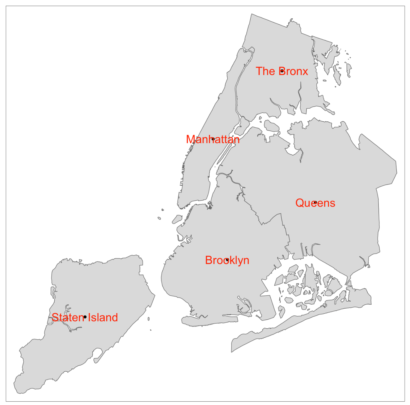 --- # Use `tmap_mode()` to change from static to interactive -- ```r tmap_mode("plot") # default my_map ```  --- # So easy to make it interactive -- ```r tmap_mode("view") # make interactive my_map # recreate plot ``` 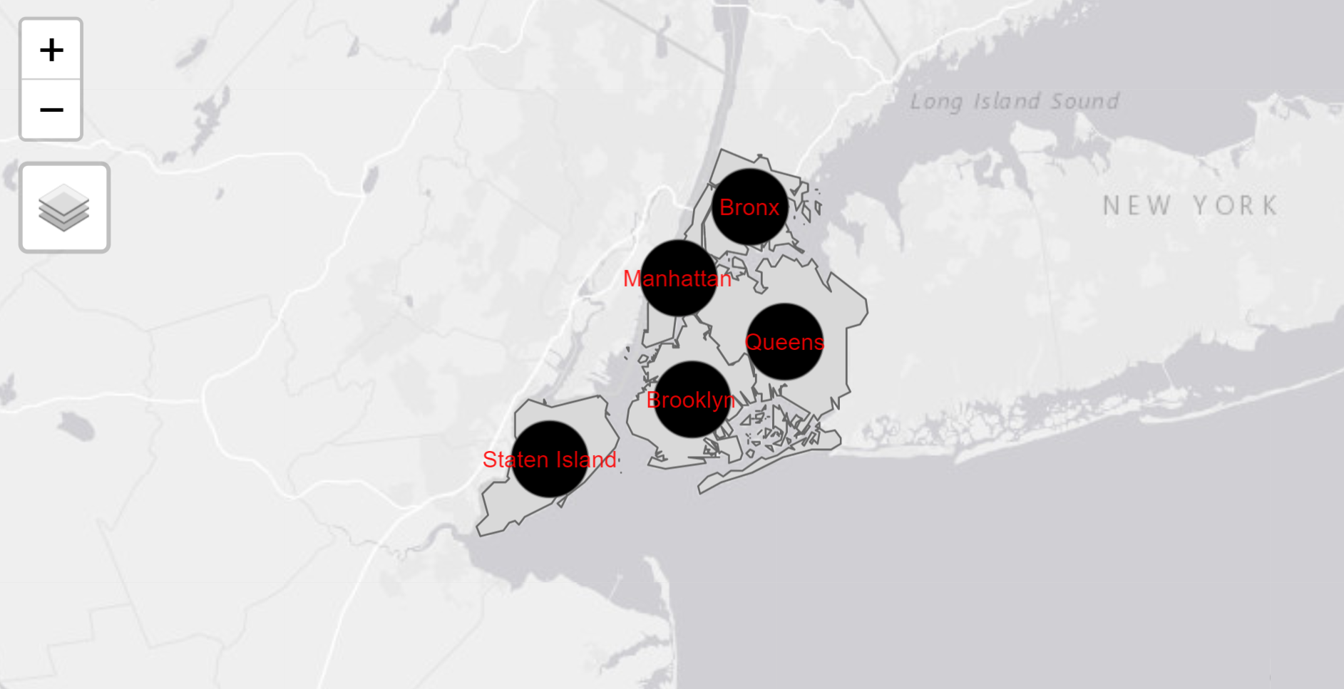 --- # Running `tmap_mode()` with no argument will give the current mode -- ```r tmap_mode() # current tmap mode is "view" ``` --- # `tmap` can do side-by-side linked plots -- ```r tmap_mode("view") tm_shape(boroughs) + tm_polygons(c("pop2018", "pop_change"), palette = "Oranges") ``` 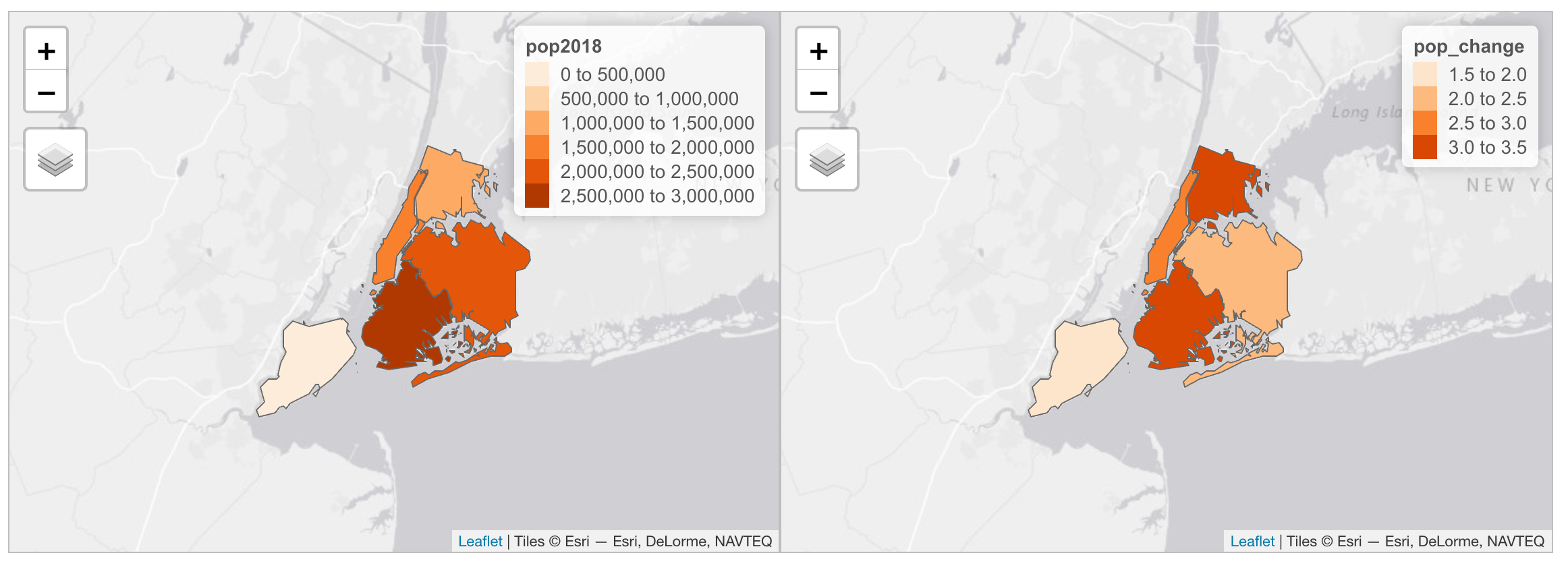 --- # Save your interactive tmap with `tmap_save()` ```r mymap <- tm_shape(boroughs) + tm_polygons() tmap_save(mymap, "mymap.html") ``` -- 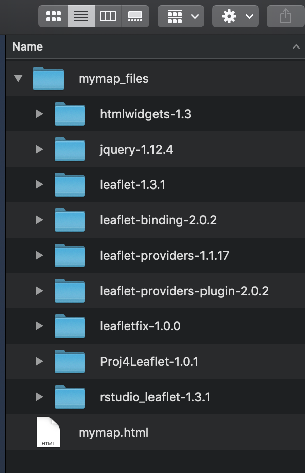 --- class: middle, center # {mapview} --- # Great for a quick interactive look at data -- ```r library(mapview) mapview(boroughs) ``` 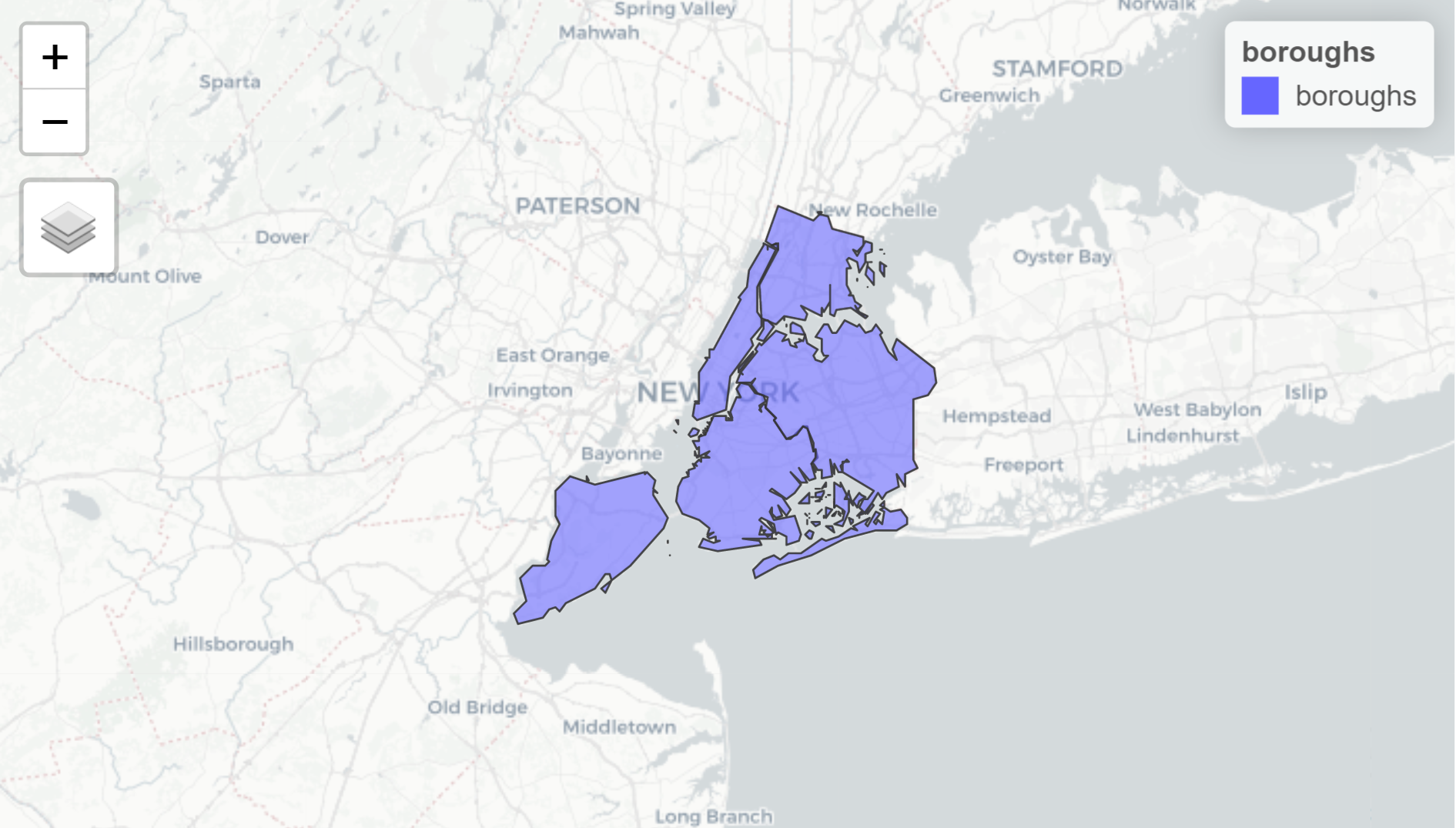 --- # Like {tmap}, a lot of customization allowed ```r mapview(x, map = NULL, maxpixels = mapviewGetOption("mapview.maxpixels"), col.regions = mapviewGetOption("raster.palette")(256), at = NULL, na.color = mapviewGetOption("na.color"), use.layer.names = FALSE, values = NULL, map.types = mapviewGetOption("basemaps"), alpha.regions = 0.8, legend = mapviewGetOption("legend"), legend.opacity = 1, trim = TRUE, verbose = mapviewGetOption("verbose"), layer.name = NULL, homebutton = TRUE, native.crs = FALSE, method = c("bilinear", "ngb"), label = TRUE, query.type = c("mousemove", "click"), query.digits, query.position = "topright", query.prefix = "Layer", viewer.suppress = FALSE, ...) ``` --- # And easier than... ```r tmap_mode("view") tm_shape(boroughs) + tm_polygons() ``` --- # Multiple layers in one map with `list()` -- ```r library(mapview) mapview(list(boroughs, schools)) ``` 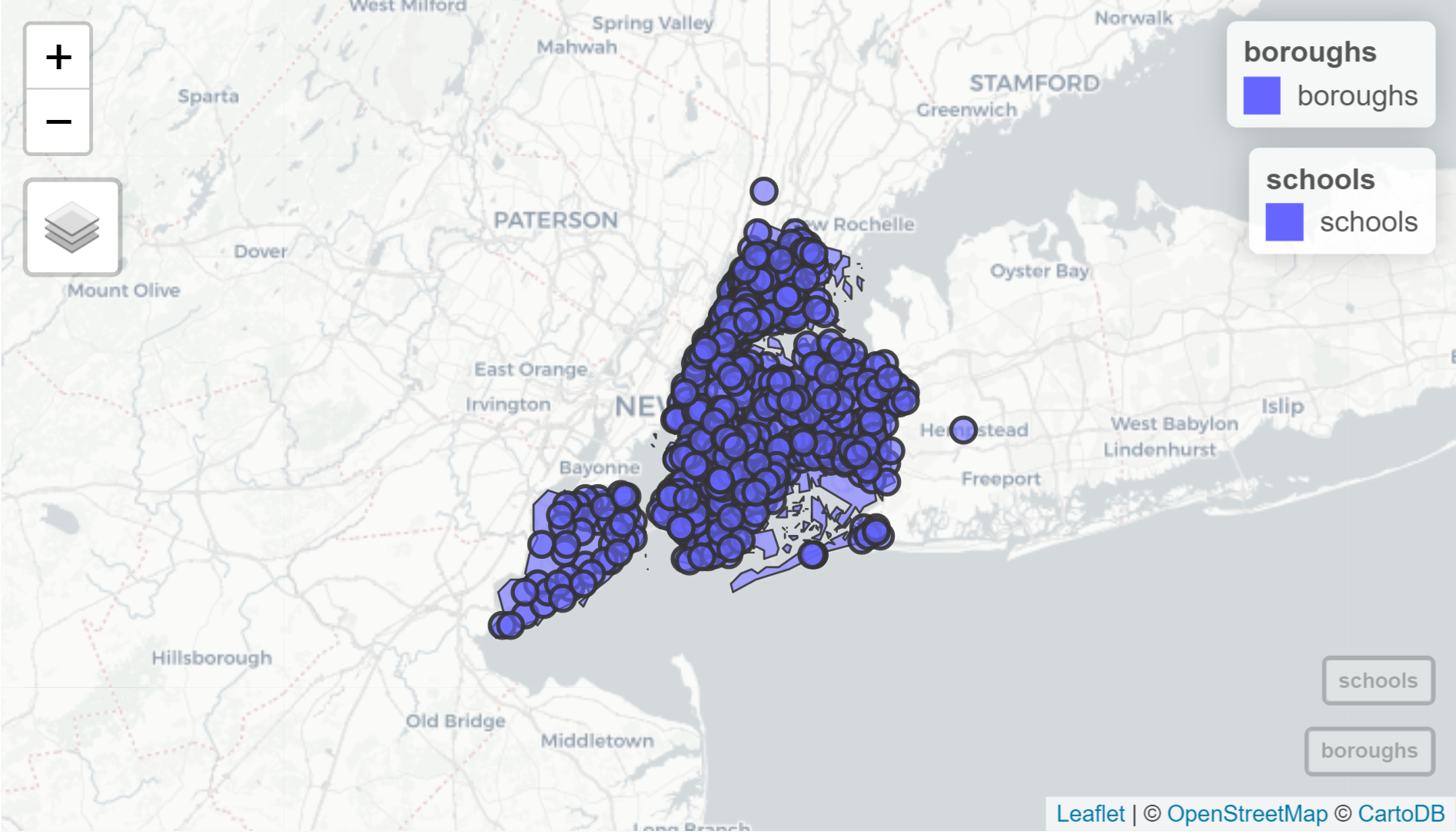 --- # Alternative syntax for multiple layers -- ```r mapview(boroughs) + mapview(schools) ``` -- ```r mapview(boroughs) + schools ``` --- # Color-code based on an attribute use the `zcol` argument ```r mapview(boroughs, zcol = "Shape_Area") ``` 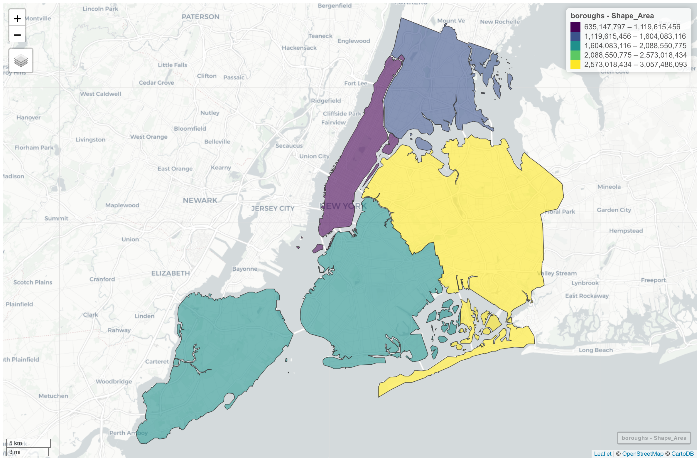 --- # Also allows rasters -- ```r mapview(canopy, alpha.regions = 0.4) ``` 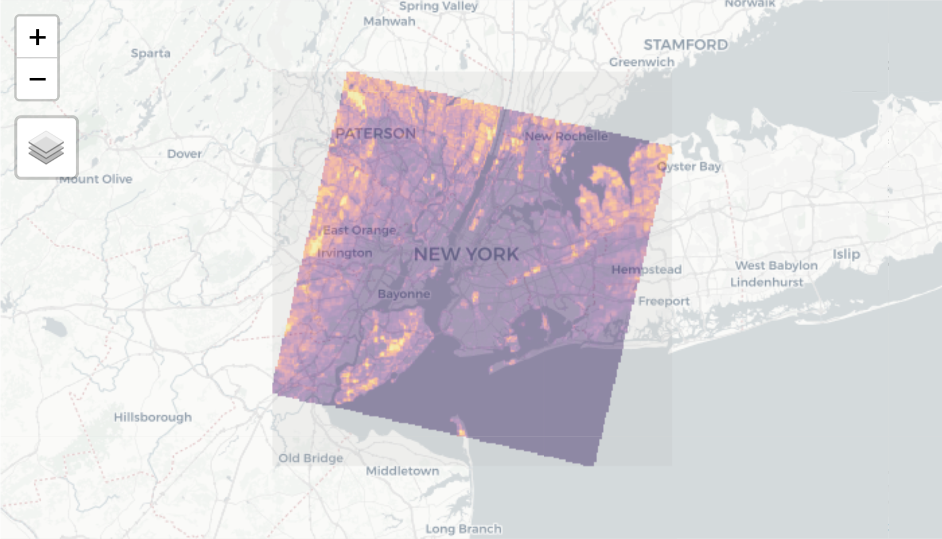 --- # Saving your mapview interactive map with `mapshot` Output is very similar to {tmap} (html file and folder) -- ```r mymap <- mapview(boroughs) mapshot(mymap, "mymap.html") ``` --- # For both static and interactive maps -- * You can include in R markdown -- * You can include in shiny application -- * If you save with `tmap_save()` or `mapshot()` you can upload the files directly to a server --- class: center, middle, doExercise # open_exercise(3) and finish