class: title-slide background-size: cover <h1 class="center middle">Getting Geospatial Data<br>Into R</h1> <h3 class="center middle"></h3> <div class="logo"></div> <div class="databird"></div> --- # Ways to get spatial data into R -- * Load external spatial files -- * Load or fetch data with specialized R packages --- # In this section I'll be showing some code I'll cover in more detail later --- background-image: url("images/background.png") background-size: cover class: center, middle, separator-slide # Reading in existing data --- # What function you use depends on the type of data -- * Read **vector** data with the {sf} package -- * Read **raster** data with the {raster} package --- class: middle, center # Reading vector data --- # For vector data use `read_sf()` from {sf} --- # You can also use `st_read()` from {sf} but `read_sf()` is more "tidy" -- * `stringsAsFactors = FALSE` * `quiet = TRUE` * `as_tibble = TRUE` --- # `read_sf()` to read many different file types * Shapefiles * Geopackages * Geojson * Even databases! --- # This makes things so much easier!  --- # A little more detail on the most common vector file types --- # Shapefiles are the most common spatial files --- # Shapefiles have been around a long time!  --- # Shapefiles can be unpleasant to work with -- * Columns can only be 10 or fewer characters -- * Inconveniently a single shapefile is represented by multiple files --- # This is one "shapefile"  .footnote[A shapefile can also have several other associated files] --- # Time to move away from shapefiles  --- # Geopackages are rapidly gaining acceptance -- * Open format -- * Just one file, technically they are a SQLite container -- * Can store multiple layers in one file --- # Geojson, spatial data for the web -- * geojson is json (javascript) with geographic attributes -- * Files can be a little larger -- * Extension is usually `.geojson` (sometimes `.json`) -- * Can only be latitude/longitude --- # One point in geojson ```js { "type": "FeatureCollection", "crs": { "type": "name", "properties": { "name": "urn:ogc:def:crs:OGC:1.3:CRS84" } }, "features": [{ "type": "Feature", "properties": { "location": "Gimme! Coffee" }, "geometry": { "type": "Point", "coordinates": [-73.995001, 40.722401] } }] } ``` --- # gimme! coffee, one of my favorites  --- # A note on topojson, another format for the web -- * Topojson is similar to geojson but stores geometries more efficiently -- * For example, a border between two countries would be stored just once. -- * `read_sf()` can also read this --- # Let's see `read_sf()` in action --- # Simple example of `read_sf()` -- ```r library(sf) boroughs <- read_sf("boroughs.shp") ``` --- # `read_sf()` has a consistent syntax -- ```r boroughs <- read_sf("boroughs.shp") boroughs <- read_sf("boroughs.geojson") boroughs <- read_sf("boroughs.gpkg") ``` --- # The result will be a {sf} table ... more details later ```r glimpse(boroughs) ``` ``` ## Observations: 5 ## Variables: 7 ## $ BoroCode <int> 1, 2, 5, 3, 4 ## $ BoroName <chr> "Manhattan", "The Bronx", "Staten… ## $ Shape_Leng <dbl> 339736.6, 397460.6, 318700.5, 576… ## $ Shape_Area <dbl> 635147797, 1182399343, 1630762350… ## $ diso <int> 1, 1, 1, 1, 1 ## $ AreaSqMile <dbl> 22.78279, 42.41274, 58.49555, 71.… ## $ geom <MULTIPOLYGON [US_survey_foot]> MULTIPO… ``` --- # You can also read from a URL directly -- ```r # Topojson usa <- read_sf("http://bit.ly/2NhznGt") ``` -- ```r # Plotting discussed later st_geometry(usa) %>% plot() ```  --- # A note on making non-spatial data spatial -- * Addresses -- * Coordinates -- * Place names --- # If you have addresses, you need to "geocode" to get coordinates -- ```r # Uses Google Maps ggmap::geocode("Hilton San Francisco Union Square") ``` -- ```r # Uses Open Street Map tmaptools::geocode_OSM("Hilton San Francisco Union Square", as.sf = TRUE) %>% glimpse() ``` ``` ## Observations: 1 ## Variables: 8 ## $ query <chr> "Hilton San Francisco Union Square" ## $ lat <dbl> 37.78573 ## $ lon <dbl> -122.4104 ## $ lat_min <dbl> 37.78519 ## $ lat_max <dbl> 37.78612 ## $ lon_min <dbl> -122.4112 ## $ lon_max <dbl> -122.4096 ## $ geometry <POINT [°]> POINT (-122.4104 37.78573) ``` --- # What if you have coordinates? You need to convert them to a spatial object with {sf} --- # Here is a table of coordinates ```r regular_table ``` ``` ## # A tibble: 2 x 4 ## id latitude longitude name ## <int> <dbl> <dbl> <chr> ## 1 1 40.7 -74.0 Empire State Building ## 2 2 40.7 -74.0 One World Trade Center ``` --- # By the way X = longitude and Y = latitude A mnemonic for latitude, longitude... -- "A lat lays flat" -- "Lat are steps on a ladder" --- # We'll cover this in more detail later but... You use `sf::st_as_sf()` to convert coordinates to an {sf} object -- ```r spatial_table <- regular_table %>% st_as_sf(coords = c("longitude", "latitude"), crs = 4326) ``` -- ```r st_geometry(spatial_table) %>% plot(cex = 2, col = "blue") ``` <img src="2-spatial-data_files/figure-html/unnamed-chunk-12-1.svg" style="display: block; margin: auto;" /> --- # How about place names? You need to link them to a spatial boundary file --- # An example with US states -- ```r # My list of place names my_states <- data.frame(NAME = c("California", "Nevada")) my_states ``` ``` ## NAME ## 1 California ## 2 Nevada ``` --- # Find an R package or spatial file with the boundaries More on this topic in a second -- ```r options(tigris_class = "sf") states <- tigris::states() ``` --- # Join your place names with the geographic file -- ```r states <- inner_join(states, my_states, by = c("NAME")) ``` -- ```r # Plot! Code explained later tm_shape(states) + tm_polygons() + tm_text("NAME", size = 2) ```  --- # Write with `write_sf()` -- ```r write_sf(spatial_table, "spatial_table.shp") write_sf(spatial_table, "spatial_table.gpkg") write_sf(spatial_table, "spatial_table.geojson") ``` --- class: middle, center # Reading raster data --- # For raster data use `raster()` and `brick()` from {raster} --- # Which to use depends on the raster -- * Use `raster()` for single-band images (e.g. elevation) -- * Use `brick()` for multi-band images (e.g. satellite data) --- # Single vs multi-band 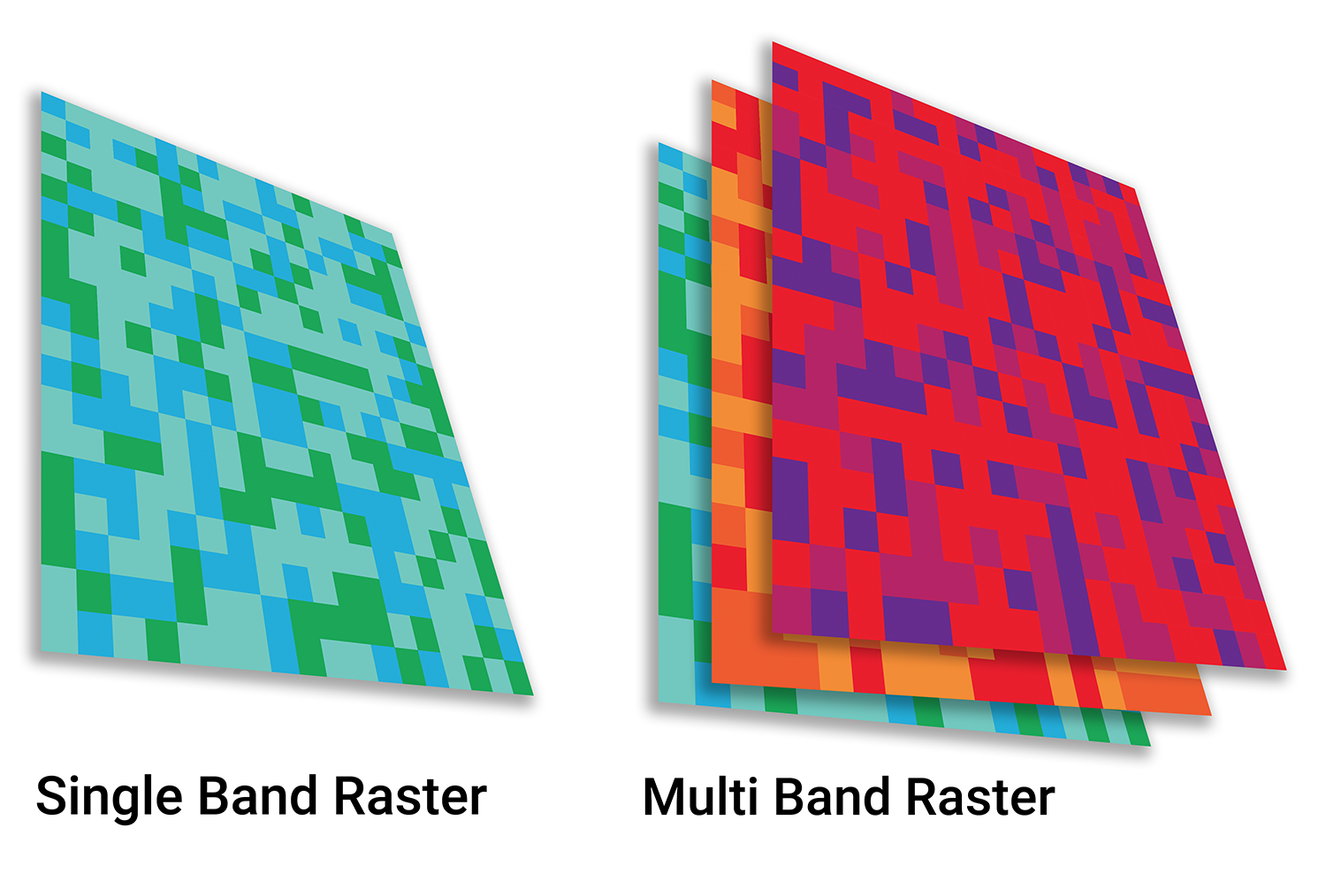 --- # Common multi-band raster -- a color image 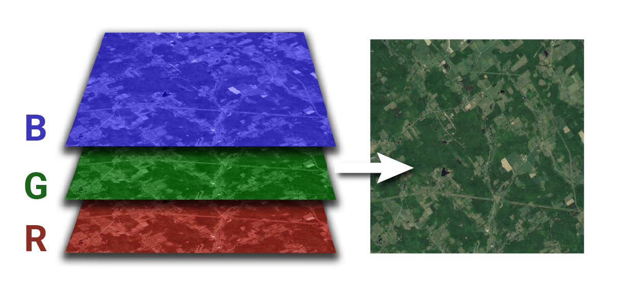 --- # Note that there is also a `stack()` function -- * A sort of "virtual" raster brick -- * Can refer to more than one file on disk -- * We will not cover this --- # `raster()` and `brick()` can read many different file types * TIFF/GeoTIFF * IMG * HDF4/5 --- # A little more detail on the most common raster file types --- # TIFF/GeoTIFF are the most common raster format -- * TIFF images can come with an extra "world" file (.tfw) -- * A TIFF with the world file embedded is a GeoTIFF -- * For storing single or multi-band rasters --- # ERDAS Imagine file * For storing single and multi-band rasters * Suffix is .img --- # HDF4/5 * Hierarchical data format for large scientific data * Multidimensional (often include both space and time and more than one image) --- # All of these formats can store single or multi-band images --- # `raster()` for single band Or to read one band from a multi-band image -- ```r library(raster) canopy <- raster("canopy.tif") ``` -- ```r plot(canopy) ``` 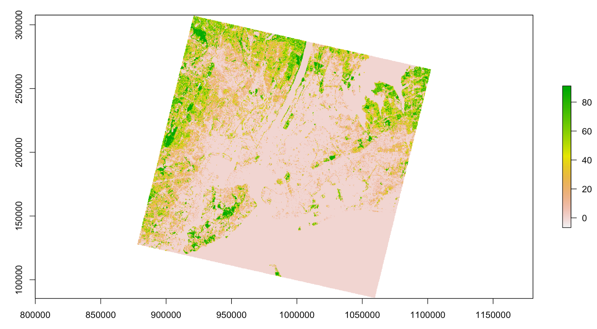 --- # `brick()` for multi-band -- ```r manhattan <- brick("manhattan.tif") ``` -- ```r plotRGB(manhattan) ``` 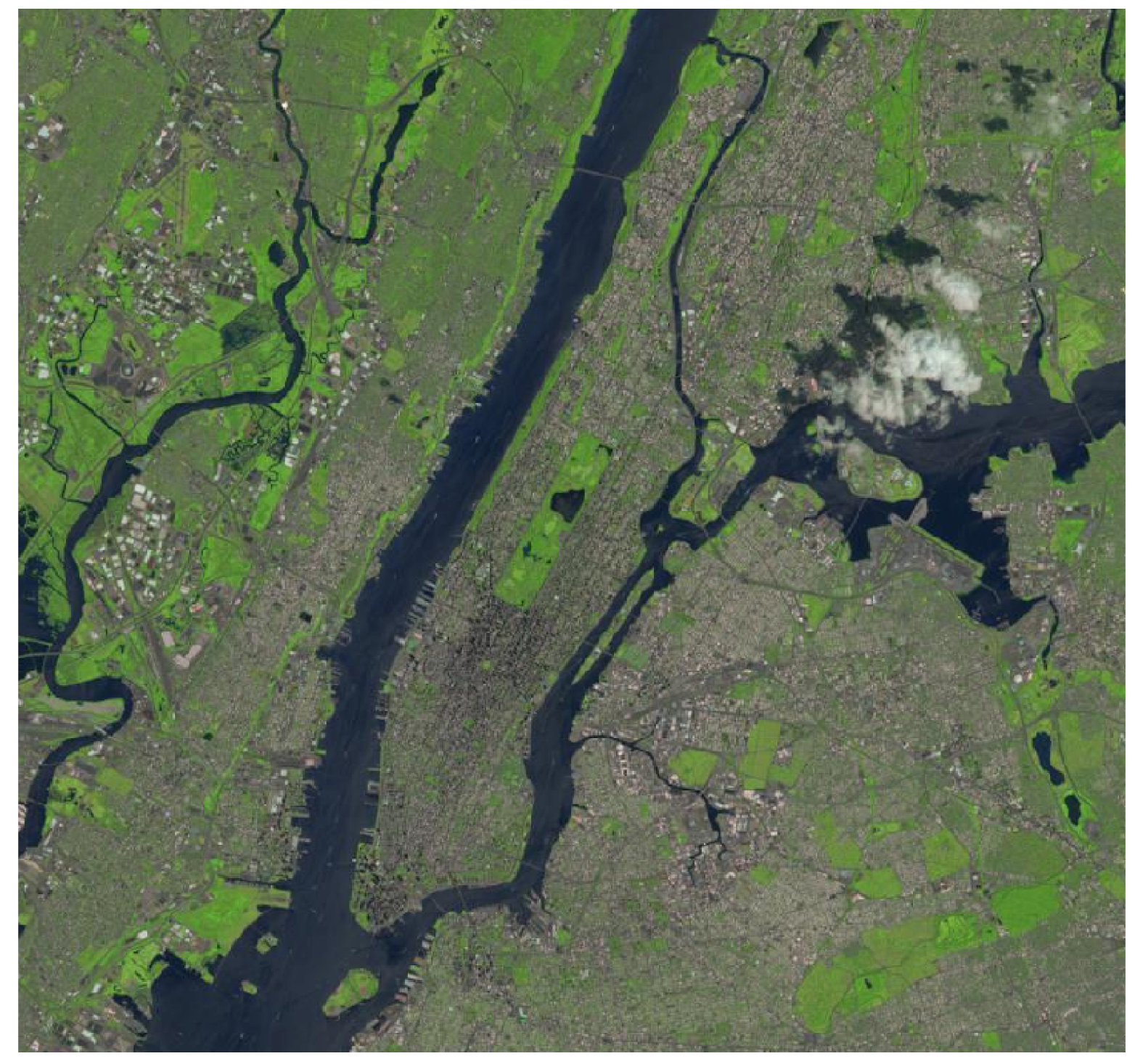 --- # Write with `writeRaster()` for both single and multi-layer files ```r writeRaster(canopy, "canopy.tif") writeRaster(canopy, "canopy.grd") ``` --- background-image: url("images/background.png") background-size: cover class: center, middle, separator-slide # R packages for getting spatial data --- # There are more than a dozen high quality packages for fetching data --- # Examples include... -- * {rnaturalearth} - country and sub-country boundaries, coastline, roads etc -- * {FedData} - mostly US-focused, elevation, landcover, climate -- * {tidycensus} - US only, census data and geography --- # Quick examples of retrieving data using R packages --- # {rnaturalearth} 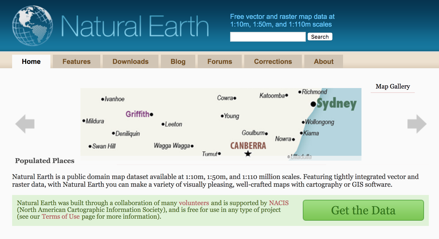 --- # {rnaturalearth} * Countries, states, airports, roads, urban areas, railroads, ocean and more * Retrieves vector data * Andy South, <https://github.com/ropensci/rnaturalearth> --- # {rnaturalearth} to get countries of the world -- ```r library(rnaturalearth) countries <- ne_countries(returnclass = "sf") ``` -- ```r # We will talk about st_geometry() in the next section st_geometry(countries) %>% plot() ``` 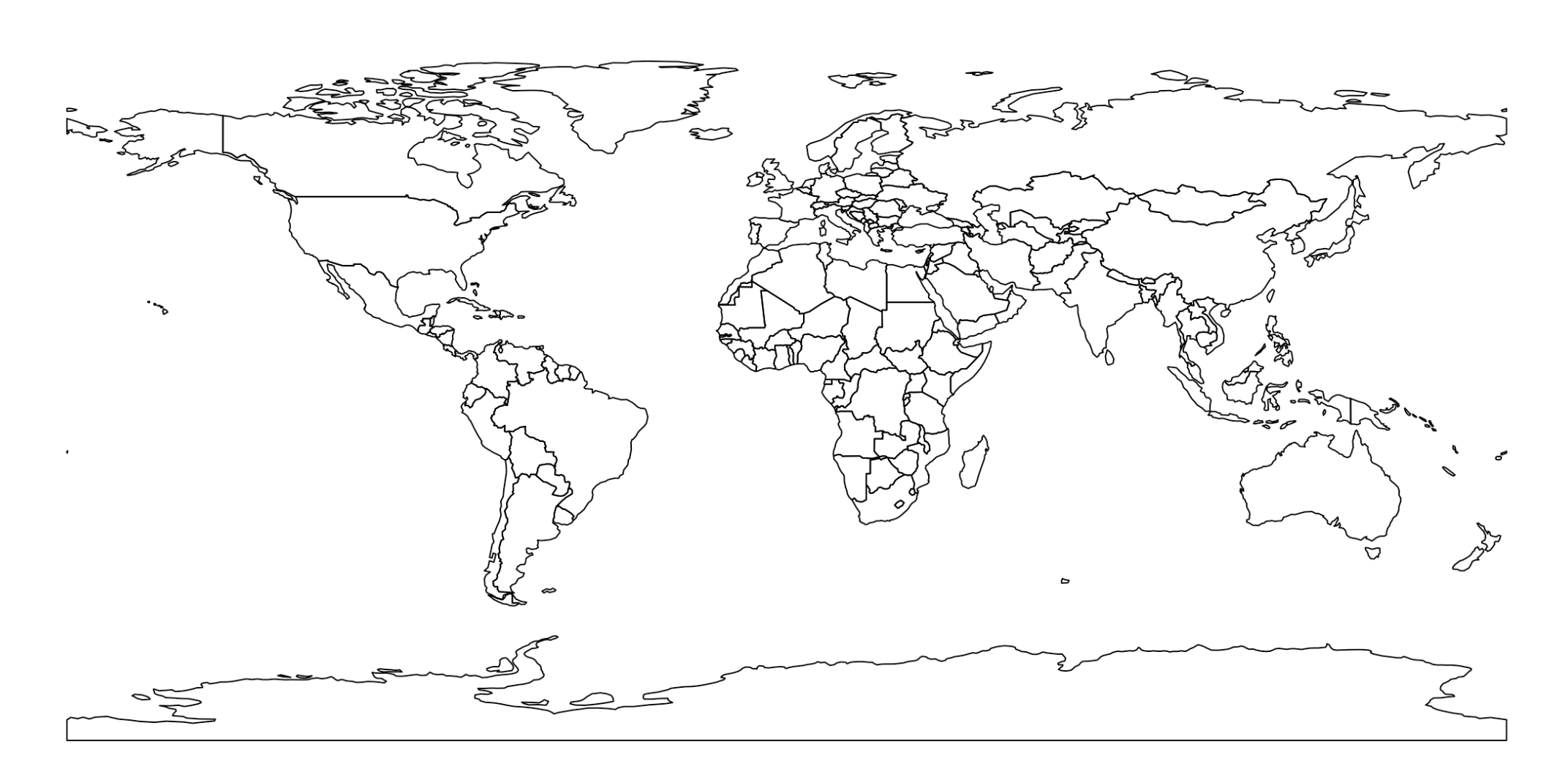 --- # {FedData} 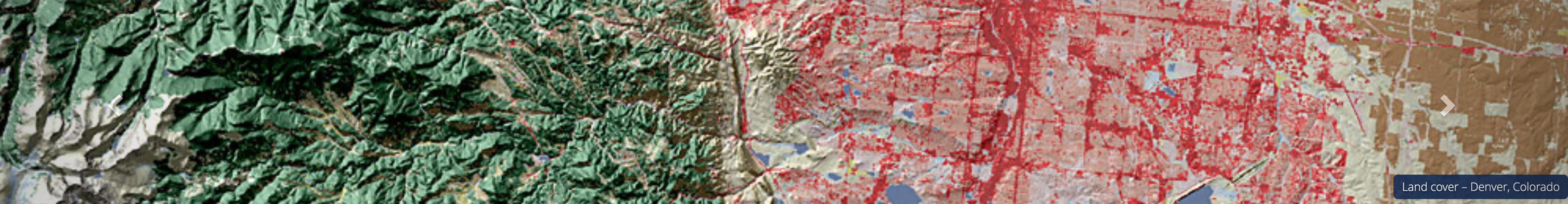 * Elevation, hydrography, soils, climate, land cover * Retrieves raster data * Kyle Bocinsky, <https://github.com/ropensci/FedData> .footnote[www.mrlc.gov] --- # {FedData} elevation in two steps -- Step 1, define your extent: ```r library(FedData) poly <- polygon_from_extent( raster::extent(672800, 740000, 4102000, 4170000), proj4string = "+proj=utm +datum=NAD83 +zone=12") ``` -- Step 2, download elevation data ```r ned <- get_ned(template = poly, label = "elevation") ``` --- # Plot the elevation data from {FedData} -- ```r raster::plot(ned) ``` 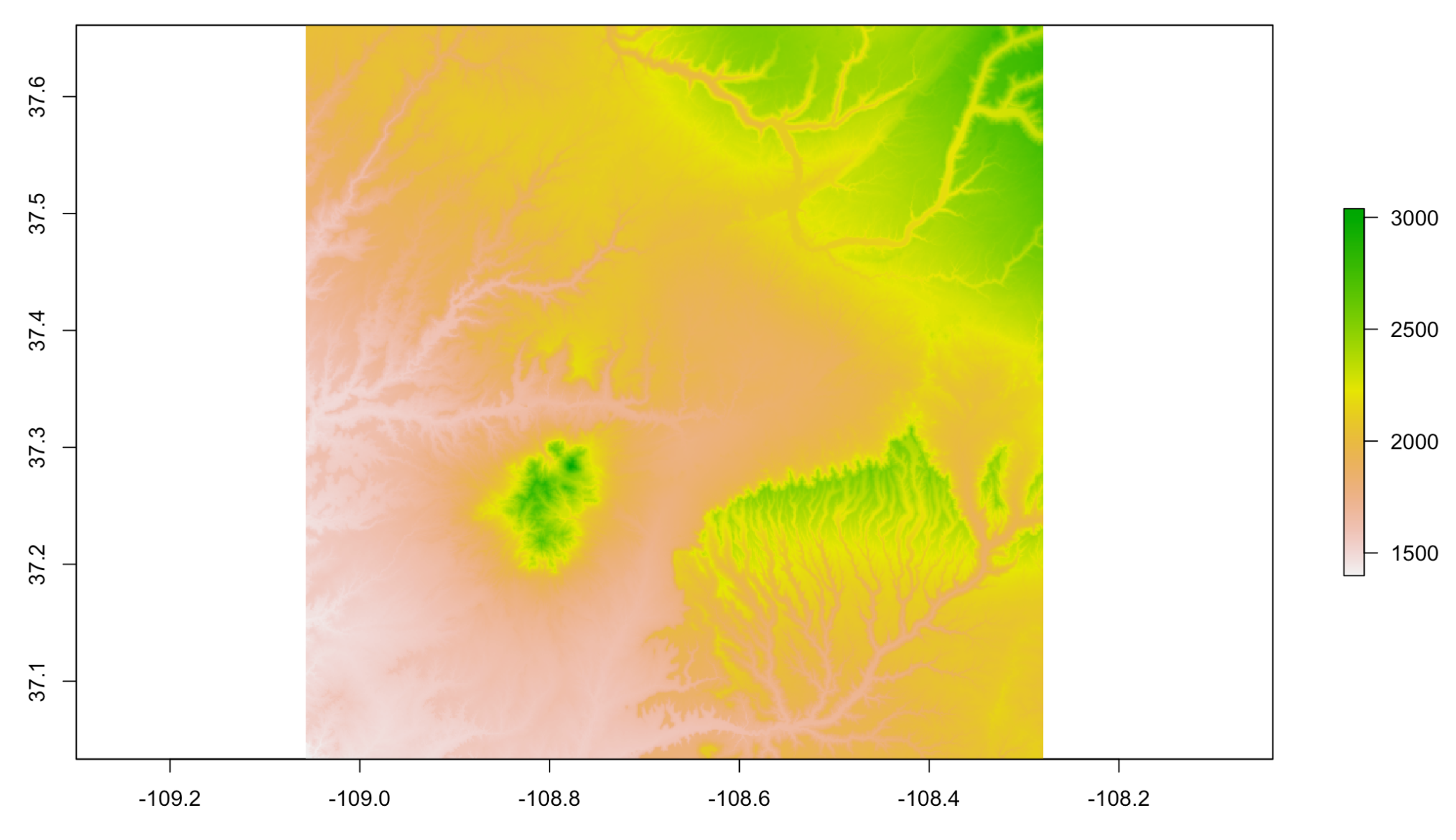 --- # {tidycensus}  .footnote[Map by Austin Wehrwein] --- # {tidycensus} * Access US Census data and geography * Super-handy for my work! * Kyle Walker, <https://github.com/walkerke/tidycensus> --- # You need an API key from the Census! * http://api.census.gov/data/key_signup.html -- * census_api_key("YOUR KEY GOES HERE") --- # If all you need is census geography you can use {tigris} instead This is what `tidycensus` uses --- # Get the data median income ```r us_county_income <- get_acs(geography = "county", variables = "B19013_001", geometry = TRUE) ``` --- # Plot the data ```r library(tmap) tm_shape(us_county_income) + tm_fill("estimate", pal = "-viridis") ```  --- class: center, middle, doExercise # open_exercise(2)