Computability, Complexity, and Algorithms
Charles Brubaker and Lance Fortnow
Computability, Complexity, and Algorithms
Charles Brubaker and Lance Fortnow
Undecidability - (Udacity)
Introduction - (Udacity, Youtube)
As a computer scientist, you have almost surely written a computer program that just sits there spinning its wheels when you run it. You don’t know whether the program is just taking a long time or if you made some mistake in the code and the program is in an infinite loop. You might have wondered why nobody put a check in the compiler that would test your code to see whether it would stop or loop forever. The compiler doesn’t have such a check because it can’t be done. It’s not that the programmers are not smart enough, or the computers not fast enough: it is just simply impossible to check arbitrary computer code to determine whether or not it will halt. The best you can do is simulate the program to know when it halts, but if it doesn’t halt, you can never be sure if it won’t halt in the future.
In this lesson we’ll prove this amazing fact and beyond, not only can you not tell whether a computer halts, but you can’t determine virtually anything about the output of a computer. We build up to these results starting with a tool we’ve seen from our first lecture, diagonalization.
Diagonalization - (Udacity, Youtube)
The diagonalization argument comes up in many contexts and is very useful for generating paradoxes and mathematical contradictions. To show how general the technique is, let’s examine it in the context of English adjectives.
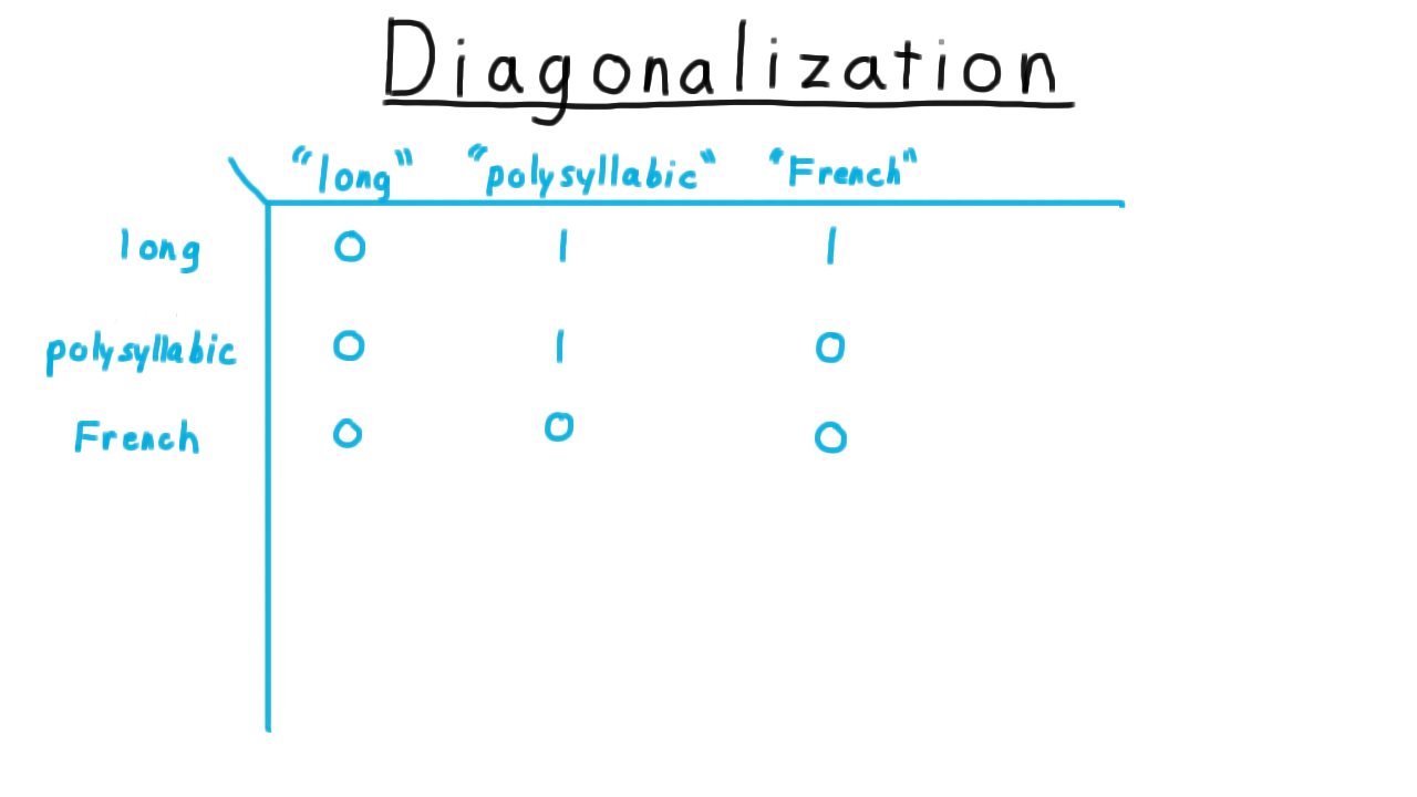
Here I’ve created a table with English adjectives both as the rows and as the columns. Consider the row to be the word itself and the column to be the string representation of the word. For each entry, I’ve written a 1 if the row adjective applies to the column representation of the word. For instance, “long” is not a long word, so I’ve written a 0. “Polysyllabic” is a long word, so I’ve written a 1. “French” is not a French word, it’s an English word, so I’ve written a 0. And so forth.
So far, we haven’t run into any problems. Now, let’s make the following definition: a heterological word is a word that expresses a property that its representation does not possess. We can add the representation to the table without any problems. It is a long, polysyllabic, non-French word. But when we try to add the meaning to the table, we run into problems. Remember: a heterological word is one that express a property that its representation does not posseses. “Long” is not a long word, so it is heterological. “Polysyllabic” is a polysyllabic word, so it is not heterological, and “French” is not a French word, so it is heterological.
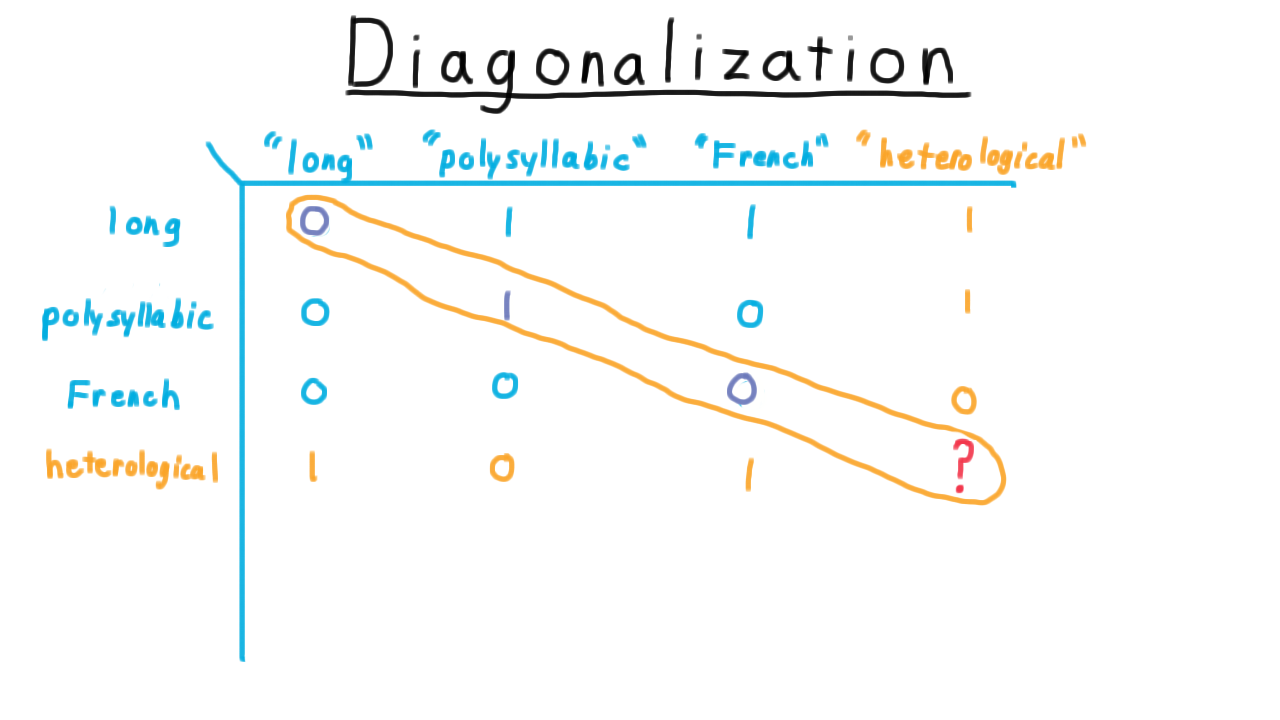
What about “heterological,” however? If we say that it is heterological (causing us to put a 1 here), then it applies to itself and so it can’t be heterological. On the other hand, if we say it is not heterological (causing us to put a zero here), then it doesn’t apply to itself and it is heterological. So there really is no satisfactory answer here. Heterological is not well-defined as an adjective.
For English adjectives, we tend to simply tolerate the paradox and politely say that we can’t answer that question. Even in mathematics the polite response was simply to ignore such questions until around the turn of the 20th century when philosophers began to look for a more solid logical foundations for reasoning and for mathematics in particular.
Naively, one might think that a set could be an arbitrary collection. But what about the set of all sets that do not contain themselves? Is this set a member of itself or not? This paradox posed by Bertrand Russell wasn’t satisfactorily resolved until the 1920s with the formulation of what we now call Zermelo-Fraenkel set theory.
Or from mathematical logic, consider the statement, “This statement is false.” If this statement is true, then it says that it is false. And if this statement is false, then it says so and should be true. It turns out that falsehood in this sense isn’t well-defined mathematically.
At this point, you’ve probably guessed where this is going for this course. We are going to apply the diagonalization trick to Turing machines.
An Undecidable Language - (Udacity, Youtube)
Here is the diagonalization trick applied to Turing machines. We’ll let \(M_1, M_2, \ldots \), be the set of all Turing machines. Turing machines can be described with strings, so there are a countable number of them and therefore such an enumeration is possible. We’ll create a table as before. I’ll define the function
\[ f(i,j) = \left\{ \begin{array}{ll} 1 & \mathrm{if} \; M_i \; \mathrm{accepts }\; < M_j > \\\\ 0 & \mathrm{otherwise} \end{array}\right. \]
For this example, I’ll fill out the table in some arbitrary way. The actual values aren’t important right now.

Now consider the language L, consisting of string descriptions of machines that do not accept their own descriptions. I.e.
\[ L = \{ < M > | < M > \notin L(M) \}. \]
Let’s add a Turing machine \(M_L\) that recognizes this language to the grid.

Again we run into a problem. The row corresponding to \(M_L\) is supposed to have the opposite values of what is on the diagonal. But what about the diagonal element of this row? What does the machine do when it is given its own description? If it accepts itself, then \(< M_L >\) is not in the language \(L\), so \(M_L\) should have accepted itself. On the other hand, if \(M_L\) does not accept its string representation, then \(< M_L >\) is in the language \(L\), so \(M_L\) should have accepted its string representation!
Thankfully, in computability, the resolution to this paradox isn’t as hard to see as in set theory or mathematical logic. We just conclude that the supposed machine \(M_L\) that recognizes the language L doesn’t exist.
Here is natural to object: “Of course, it exists. I just run M on itself and if it doesn’t accept, we accept.” The problem is that M on itself might loop, or it just might run for a very long time. There is no way to tell the difference.
The end result, then, is that the language L of string descriptions of machines that do not accept their own descriptions is not recognizable.
Recall that in order for a language to be decidable, both the language and its complement have to be recognizable. Since L is not recognizable, it is not decidable, and neither is it’s complement, the language where the machine does accept its own description. We’ll call this D_TM, D standing for diagonal,
\[D_{TM} = \{ < M > | < M > \in L(M)\} \]
These facts are the foundation for everything that we will argue in this lesson, so please make sure that you understand these claims.
Dumaflaches - (Udacity)
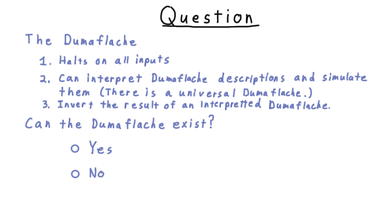
If you think back to the diagonalization of Turing machines, you will notice that we hardly referred to the properties of Turing machines at all. In fact, except at the end, we might as well have been talking about a different model of computation, say the dumaflache. Perhaps, unlike Turing machines, dumaflaches halt on every input. These models exist. A model that allowed one step for each input symbol would satisfy this requirement.
How do we resolve the paradox then? Can’t we just build a dumaflache that takes the description of a dumaflache as input and then runs it on itself? It has to halt, so we can reject it if accepts and accept if it rejects, achieving the needed inversion. What’s the problem? Take a minute to think about it.
Mapping Reductions - (Udacity, Youtube)
So far, we have only proven that one language is unrecognizable. One technique for finding more is mapping reduction, where we turn an instance of one problem into an instance of another.
Formally, we say
A language \(A\) is mapping-reducible to a language \(B\) ( \(A \leq_M B\) ) if there is a computable function \(f\) where for every string \(w\),
\[w \in A \Longleftrightarrow f(w) \in B.\]
We write this relation between languages with the less-than-or-equal-to sign with a little M on the side to indicate that we are referring to mapping reducibility.
It helps to keep in your mind a picture like this.
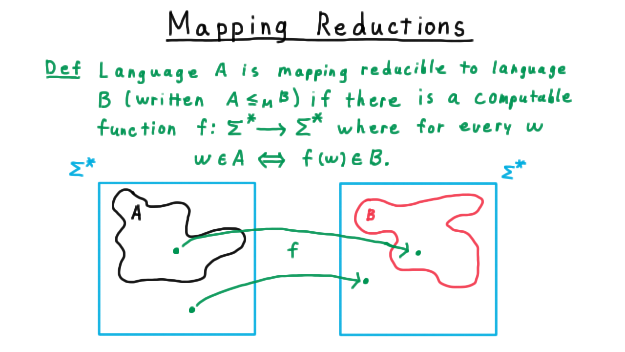
On the left, we have the language \(A\), a subset of \(\Sigma^*\) and the right we have the language \(B\), also a subset of \(\Sigma^*\).
In order for the computable function \(f\) to be a reduction, it has to map
- each string in \(A\) to a string in \(B\).
- each string not in \(A\) to a string not in \(B\).
The mapping doesn’t have to be one-to-one or onto; it just has to have this property.
Some Trivial Reductions - (Udacity, Youtube)
Before using reductions to prove that certain languages are undecidable, it sometimes helps to get some practice with the idea of a reduction itself–as a kind of warm-up. With this in mind, we’ve provided a few programming exercises. Good luck!
EVEN <= {’Even’} - (Udacity)
{’John‘} <= Complement of {’John’} - (Udacity)
{’Jane’} <= HALT - (Udacity)
Reductions and (Un)decidability - (Udacity, Youtube)
Now that we understanding reductions, we are ready to use them to help us prove decidability and even more interestingly undecidability.
Suppose then that we have a language \(A\) that reduces to \(B\) (i.e. \( A\leq_M B\) ), and, let’s say that I want to know whether some string \(x\) is in \(A\).
If there is a decider for \(B\), then I’m in luck. I can use the reduction, which is a computable function, that takes in the one string and outputs another. I just need to feed in \(x\), take the output, and feed that into the decider for \(B\). If \(B\) accepts, then I know that \(x\) is in \(A.\) If \(B\) rejects, then I know that it isn’t.
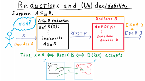
This works because by the definition of a reduction \(x\) is in \(A\) if and only if \(R(x)\) is in \(B\). And by the definition of a decider this is true if and only if \(D\) accepts \(R(x)\). Therefore, the output of \(D\) tells me whether \(x\) is in \(A.\) If I can figure out whether an arbitrary string is in \(B\), then by the properties of the reduction, this also lets me figure out whether a string is in \(A\). We can say that the composition of the reduction with the decider for \(B\) is itself a decider for \(A.\)
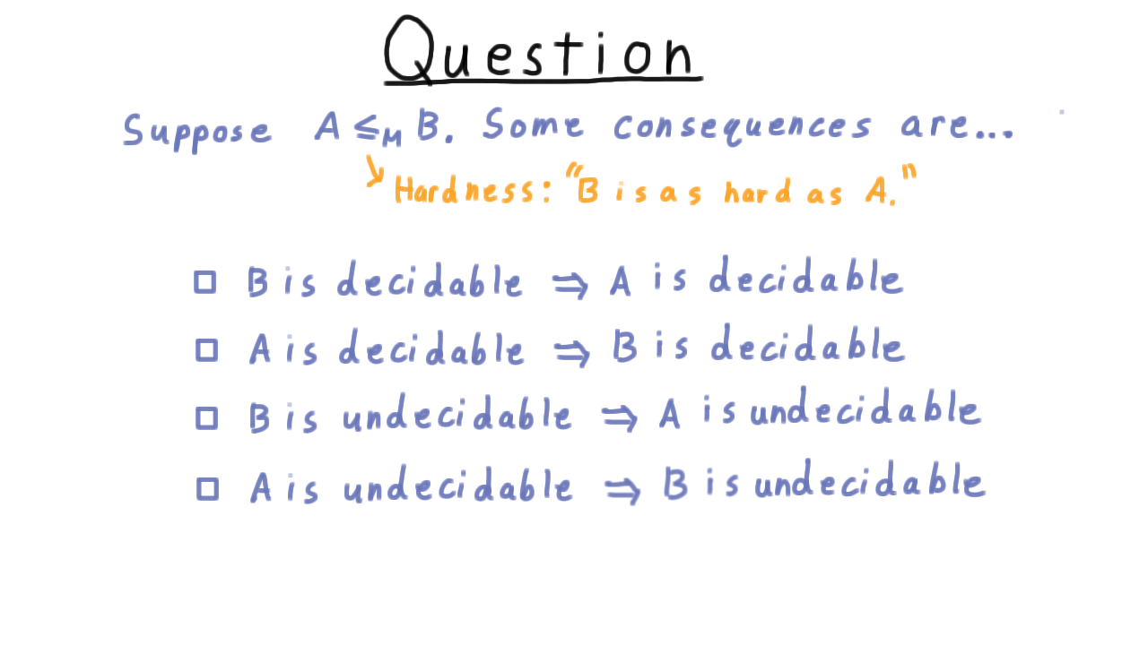
Thus, the fact that \(A\) reduces to \(B\) has four important consequences for decidability and recognizability. The easiest to see are
- If \(B\) is decidable, then \(A\) is also decidable. (As we’ve seen we can just compose the reduction with the decider for \(B.\))
- If \(B\) is recognizable, then \(A\) is also recognizable. (Same logic as above.)
The other two consequences are just the contrapositives of these.
- If \(A\) is undecidable, then B is undecidable. (This composition of the reduction and the decider for B can’t be a decider. Since we are assuming that there is a reduction, the only possibility is that the decider for B doesn’t exist. Hence, B is undecidable.)
- If \(A\) is unrecognizable, then B is unrecognizable. (Same logic as above)
Remember the Consequences - (Udacity)
Let’s do a quick question on the consequences of there being a reduction between two languages.
A Simple Reduction - (Udacity, Youtube)
Now we are going to use a simple reduction to show that the language \(B\), consisting of the descriptions of Turing machines that accept something, i.e.
\[ B = \{ < M > | \; L(M) \neq \emptyset \},\]
is undecidable.
Our strategy is to reduce the diagonal language to it. In other words, we’ll argue that deciding \(B\) is at least as hard as deciding the diagonal language. Since we can’t decide the diagonal language, we can’t decide \(B\) either.
Here is one of many possible reductions.
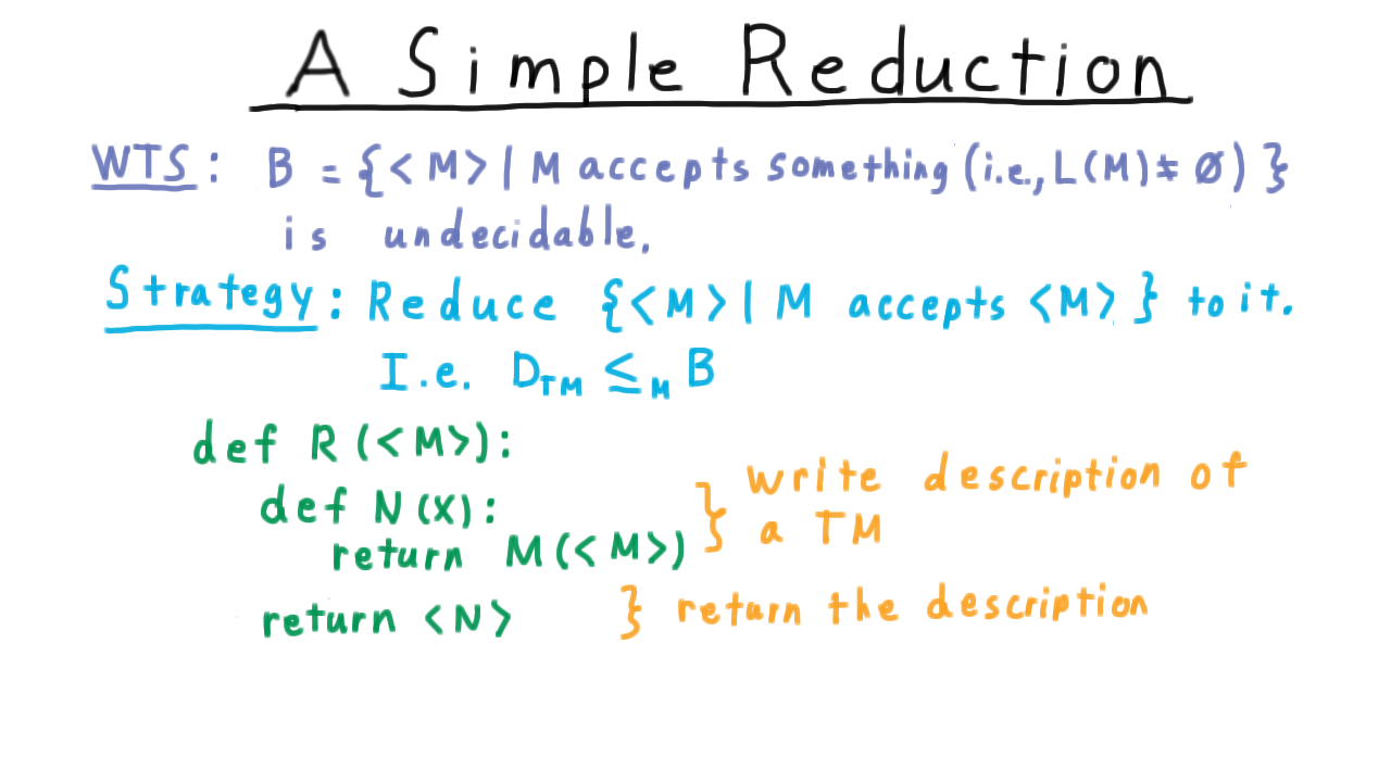
The reduction is a computable function whose input is the description of a machine M, and it’s going to build another machine N in this python-like notation. First, we write down the description of a Turing machine by defining this nested function. Then we return that function. An important point is that the reduction never runs the machine N: it just writes the program for it!
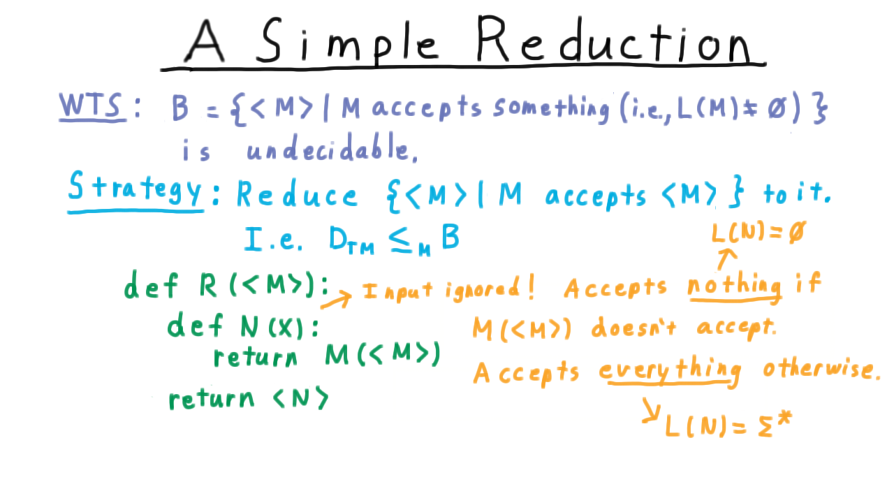
Note here that, in this example, N totally ignores the actual input that is given to it. It just accepts if M(
In other words, the language of N will be the empty set in one case and Sigma-star in the other. A decider for B would be able to tell the difference, and therefore tell us whether M accepted its own description. Therefore, if B had a decider, we would be able to decide the diagonal language, which is impossible. So B cannot be decidable.
The Halting Problem - (Udacity, Youtube)
Next, we turn to the question of halting. As we have seen, not being able to tell whether a program will halt or not plays a central role in the diagonalization paradox, and it is at least partly intuitive that we can’t tell whether a program is just taking a long time or if it will run forever. It shouldn’t be surprising, then, that given an arbitrary program-input pair, we can’t decide whether the program will halt on that input. But actually, the situation is much more extreme. We can’t even decide if a program will halt when it is given no input at all: just the empty string.
Let’s go ahead prove this:
The language of descriptions of Turing machines that halt on the empty string, i.e.
\[ H_{TM} = \{ < M > |\; M \; \mathrm{halts}\; \mathrm{on} \; \epsilon\}\]
is undecidable.
We’ll do this by reducing from the diagonal language. That is, we’ll show the halting problem is at least as hard as the diagonal problem. Here is one of many possible reductions.
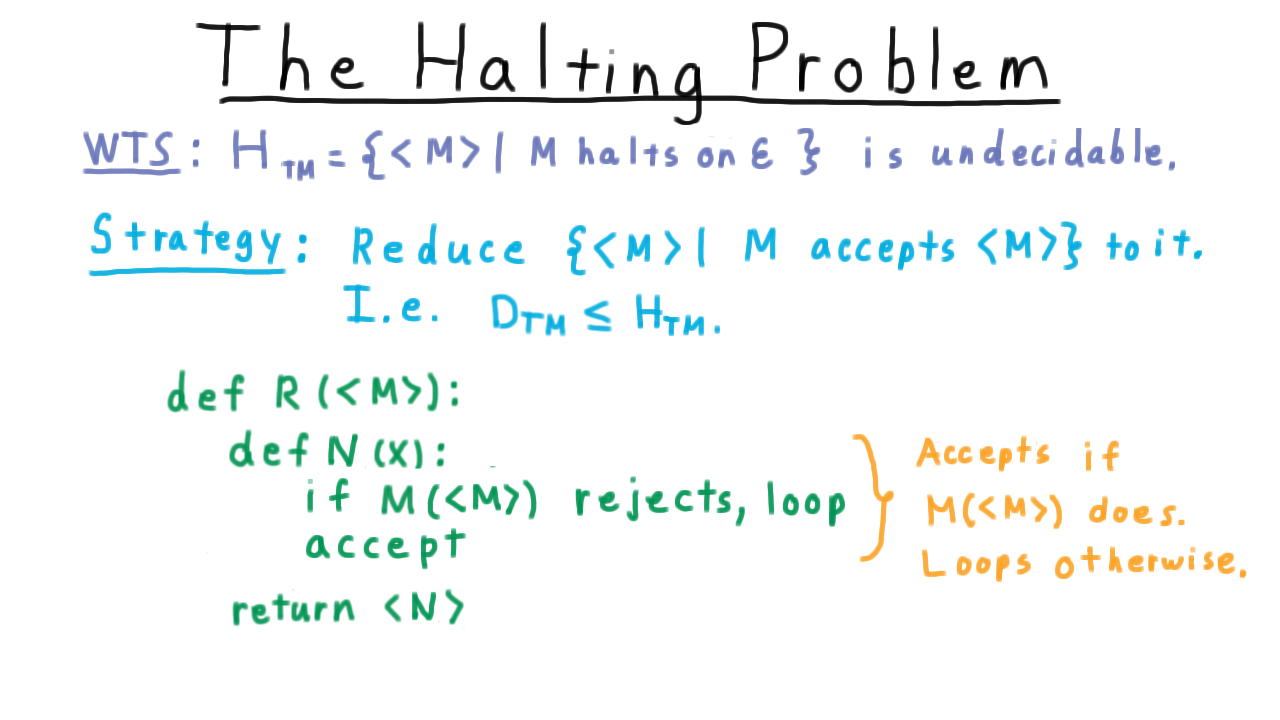
The reduction creates a machine N that simply ignores its input and runs M on itself. If M rejects itself, then N loops. Otherwise, N accepts.
At this point it might seem we’ve just done a bit of symbol manipulation but let’s step back and realize what we’ve just seen. We showed that no Turing machine can tell whether or not a computer program will halt or remain in a loop forever. This is a problem that we care about it and we can’t solve it on a Turing machine or any other kind of computer. You can’t solve the halting problem on your iPhone. You can’t solve the halting problem on your desktop, no matter how many cores you have. You can’t solve the halting problem in the cloud. Even if someone invents a quantum computer, it won’t be able to solve the halting problem. To misquote Nick Selby: “If you want to solve the halting problem, you’re at Georgia Tech but you still can’t do that!”
Filtering - (Udacity, Youtube)
So far, the machines we’ve made in our reductions (i.e. the \(N\)s) have been relatively uncomplicated: they all either accepted every string or no strings. Unfortunately, reductions can’t always be done that way, since the machine that always loops and the machine that always accepts might both be in or both not be in the language we’re reducing to. In these cases, we need \(N\) to pay attention to its input. Here is an example where we will need to do this: the language of descriptions of Turing machine where the Turing machine accepts exactly one string, i.e.
\[ S = \{ < M > |\; |L(M)| = 1 \}. \]
It doesn’t make much of a difference which undecidable language we reduce from, so this time we will reduce from the halting problem to \(S\). Again, there are many possible reductions. Here is one.
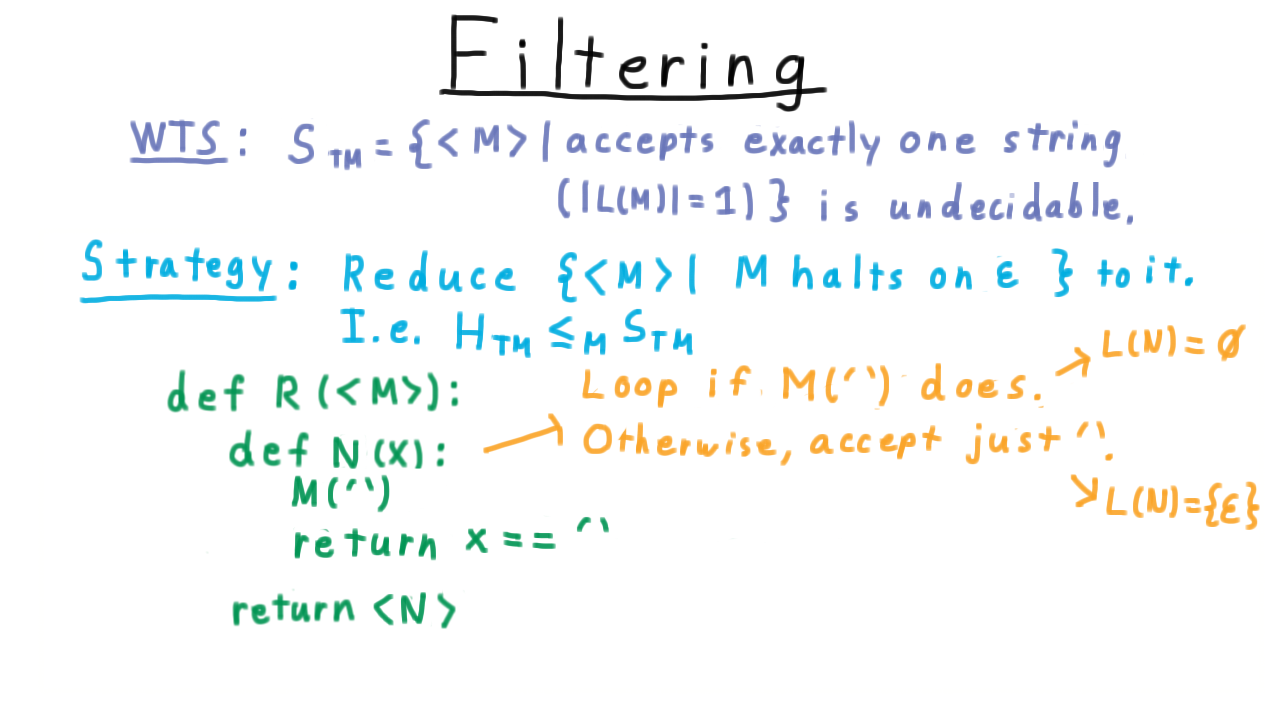
We run the input machine \(M\) on the empty string. If \(M\) loops, then so will \(N\). We don’t accept one string, we accept none. On the other hand, if \(M\) does halt on the empty string, then we make \(N\) act like a machine in the language \(S.\) The empty string is as good as any, so we’ll test to see if \(N\)’s input \(x\) is equal to that and accept or reject accordingly. This works because if \(M\) halts on the empty string, then \(N\) accepts just one string–the empty one–and so is in \(S\). On the other hand, if M doesn’t halt on the empty string, then N won’t halt on (and therefore won’t accept) anything, and therefore N isn’t in L.
In the one case, the language of \(N\) is the empty string. In the other case, the language of \(N\) is the empty set. A decider for the language \(S\) can tell the difference, and therefore we’d be able to decide if \(M\) halted on the empty string or not. Since this is impossible, a decider for \(S\) cannot exist.
Not Thirty-Four - (Udacity)
Now you get a chance to practice doing reductions on your own. I’ve been using a python-like syntax in the examples, so this shouldn’t feel terribly different. I want you to reduce the language LOOP to the language L of Turing machines that do not accept 34 in binary.
As we’ll see later in the lesson, it’s not possible for the Udacity site to perfectly verify your software, but if you do a straightforward reduction, then you should pass the tests provided.
\(0^n 1^n\) - (Udacity)
Now for a slightly more challenging reduction. Reduce \(H_\{™\}\) to the language L of Turing machines that accept strings of the form \(0^n1^n\).
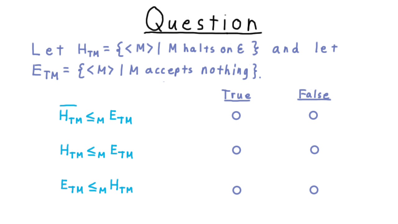
Which Reductions Work? - (Udacity)
We’ve seen a few examples, and you’ve practiced writing reductions of your own at this point. Now, I want you to test your understanding by telling me which of the following statements about these two languages is true. Think very carefully.
Rice’s Theorem - (Udacity, Youtube)
Once you have gained enough practice, these reductions begin to feel a little repetitive and it’s natural to wonder whether there is a theorem that would capture them all. Indeed, there is, and it is traditionally called Rice’s theorem after H.G. Rice’s 1953 paper on the subject. This is a very powerful theorem, and it implies that we can’t say anything about a computer just based on the language that it recognizes.
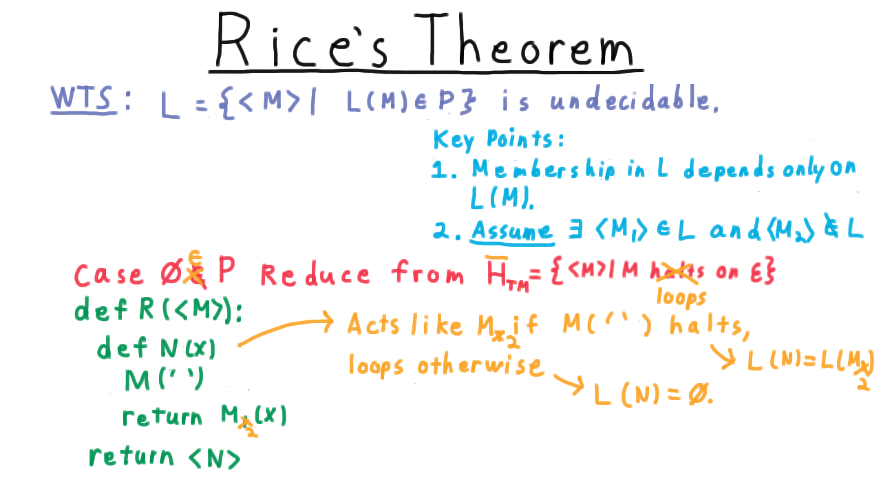
So far, the pattern has been that we have wanted to show that some language \(L\) was undecidable, where this language \(L\) was about descriptions of Turing machines whose language has certain property. It’s important to note here that the language \(L\) can’t depend on the machine \(M\) itself, only on the language it recognizes.
Two important things have been true about this language.
- Membership can only depend on the set of strings accepted by M, not about the machine M itself–like the number of states or something like that.
- The language can’t be trivial, either including or excluding every Turing machine. We’ll assume that there is a machine, \(M_1\), in the language and another, \(M_2\), outside the language.
Recall that in all our reductions, we created a machine \(N\) that either accepts nothing or else it has some other behavior depending on the behavior of the input machine \(M.\)
Similarly, there are two cases for Rice’s theorem: either the empty set is in P and therefore every machine that doesn’t accept anything is in the language L, or else the empty set is not in P. Let’s look at the case where the empty set is not in P first.

In that case, we reduce from \(H_{TM}\). The reduction looks like this. \(N\) just runs \(M\) with empty input. If \(M\) halts, then we define \(N\) to act like the machine \(M_1.\)
Thus, \(N\) acts like \(M_1\) (a machine in the language \(L\)) if \(M\) halts on the empty string, and loops otherwise. This is exactly what we want.
Now for the other case, where the empty set is in P.
In this case, we just replace \(M_1\) by \(M_2\) in the definition of the reduction, so that \(N\) behaves like \(M_2\) if \(M\) halts on the empty string.
This is fine, but we need to reduce from the complement of \(H_{TM}\): that is, from the set of descriptions of machines that loop on the empty input. Otherwise, we would end up accepting when we wanted to not accept and vice-versa.
All in all then, we have proved the following theorem.

Slightly more intuitively, we can say the following. Let \(L\) be a subset of strings representing Turing machines having two key properties:
- if \(M_1\) and \(M_2\) accept the same set of strings, then their descriptions are either both in or both out of the language–this just says that the language only depends on the behavior of the machine not its implementation.
- the language can’t be trivial–there must be a machine whose description is in the language and a machine whose description is not in the language.
If these two properties hold true, then the language is be undecidable.
Undecidable Properties - (Udacity)
Using Rice’s theorem, we now have a quick way of detecting whether certain questions are decidable. Use your knowledge of the theorem to indicate which of the following properties is decidable. For clarity’s sake, let’s say that a virus is a computer program that modifies the data on the hard disk in some unwanted way.

Conclusion - (Udacity, Youtube)
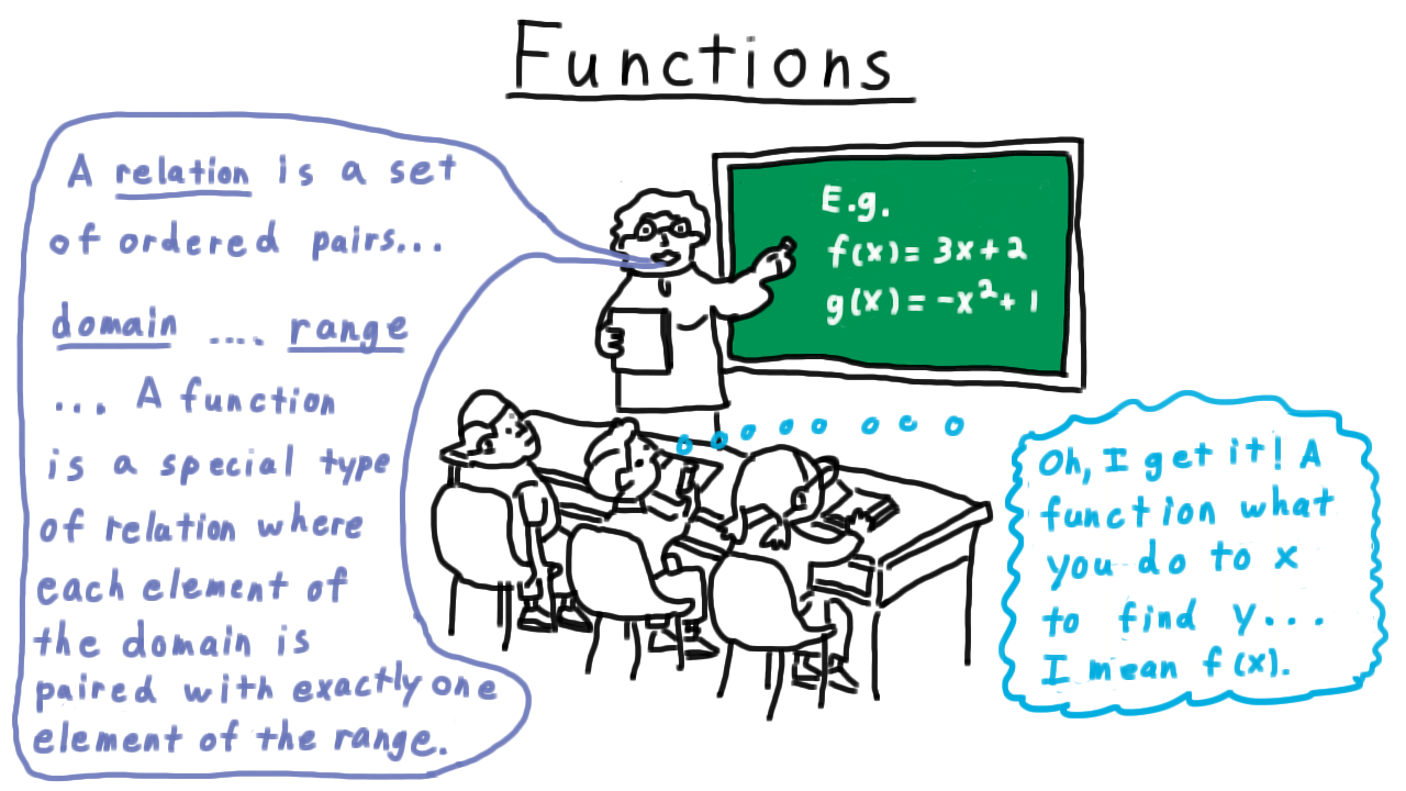
I want to end this section on computability by revisiting the scene we used at the beginning of the course, where the teacher was explaining functions in terms of ordered pairs, and the students were thinking of what they had to do to x to get y.
The promise of our study of computability was to better appreciate the difference between these understandings, and I hope you will agree that we have achieved that. We have seen how there are many functions that are not computable in any ordinary sense of the word by a counting argument. We made precise what we meant by computation, going all the way back to Turing’s inspiration from his own experience with pen and paper to formalize the Turing machine. We have seen how this model can compute anything that any computer today or envisioned for tomorrow can. And lastly, we have described a whole family of uncomputable functions through Rice’s theorem.
Towards Complexity - (Udacity, Youtube)
Even since the pioneering work of Turing and his contemporaries such as Alonzo Church and Kurt Godel, mathematical logicians have studied the power of computation and connecting it to provability as well as giving new insights on the nature of information, randomness, even philosophy and economics. Computability has a downside, just because we can solve a problem on a Turing machine doesn’t mean we can solve it quickly. What good is having a computer solve a problem if our sun explodes before we get the answer?
So for now we leave the study of computable functions and languages and move to computational complexity, trying to understand the power of efficient computation and the famous P versus NP problem.