Computability, Complexity, and Algorithms
Charles Brubaker and Lance Fortnow
Computability, Complexity, and Algorithms
Charles Brubaker and Lance Fortnow
Turing Machines - (Udacity)
Motivation - (Udacity, Youtube)
In the last lesson we talked informally about what it means to be computable. But what even is a computer? What kinds of problem can we solve on a computer? What problem can’t be solved?
To answer these questions we need a model of computation. There are many, many ways we could define the notion of computability–ideally something simple and easy to describe, yet powerful enough so this model can capture everything any computer can do, now or in the future.
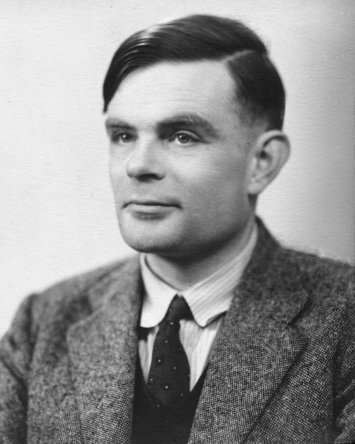
Luckily one of the very first mathematical model of a computer serves us quite well, a model developed by Alan Turing in the 1930’s. Decades before we had digital computers, Turing developed a simple model to capture the thinking process of a mathematician. This model, which we now call the Turing machine, is an extremely simple device and yet completely captures our notion of computability.
In this lesson we’ll define the Turing machine, what it means for the machine to compute and either accept or reject a given input. In future lessons we’ll use this model to give specific problems that we cannot solve.
Introduction - (Udacity, Youtube)
In the last lesson, we began to define what computation is with the goal of eventually being precise about what it can and cannot do. We said that the input to any computation can be expressed as a string, and we assumed that, whatever instructions there were for turning the input into output, that these too could be expressed as a string. Using a counting argument, we were able to show that there were some functions that were not computable.
In this lesson, we are going to look at how input gets turned into output more closely. Specifically, we are going to study the Turing machine, the classical model for computation. As we’ll see in a later lesson, Turing machines can do everything that we consider as computation, and because of their simplicity, they are a terrific tool for studying computation and its limitations. Massively parallel machines, quantum computers they can’t do anything that a Turing machine can’t also do.
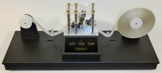
Turing machines were never intended to be practical, but nevertheless several have been built for illustrative purposes, including this one from Mike Davey.
The input to the machine is a tape onto which the string input has been written. Using a read/write head the machine turns input into output through a series of steps. At each step, a decision is made about whether and what to write to the tape and whether to move it right or left. This decision is based on exactly two things:
- the current symbol under the read-write head, and
- something called the machines state, which also gets updated as the symbol is written.
That’s it. The machine stops when it reaches one of two halting states named accept and reject. Usually, we are interested in which of these two states the machine halts in, though when we want to compute functions from strings to strings then we pay attention to the tape contents instead.
It’s a very interesting historical note that in Alan Turing’s 1936 paper in which he first proposed this model, the inspiration does not seem to come from any thought of a electromechanical devise but rather from the experience of doing computations on paper. In section 9, he starts from the idea of a person who he call the computer working with pen and paper, and then argues that his proposed machine can do what this person does.
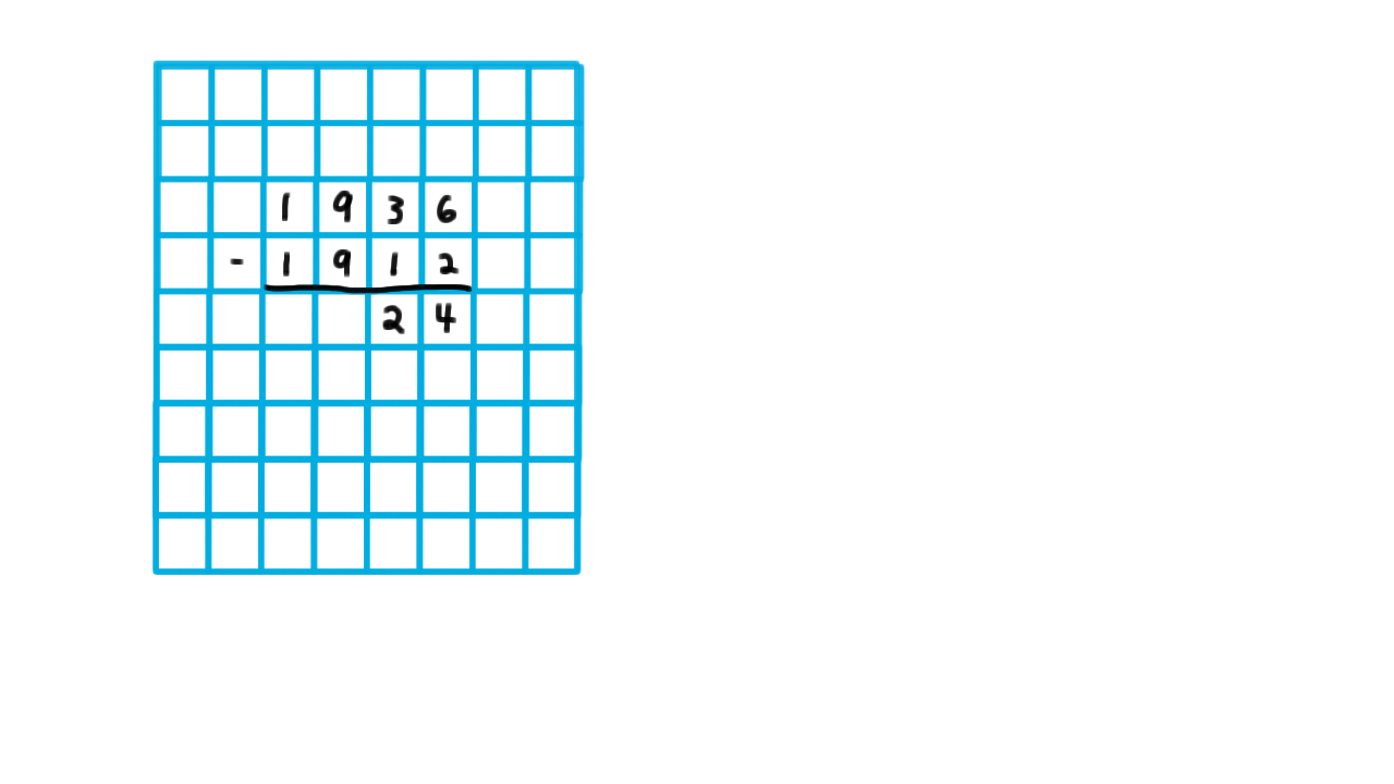
Let’s follow his logic by considering my computing a very simple number: Alan Turing’s age when he wrote the paper.
\[1936 - 1912 = 24.\]
Turing argues that any calculation like this can be done on a grid. Like a child arithmetic book, he says. By this he means something like wide-ruled graph paper. He argues that all symbols can be made to fit inside of one of these squares.
Then he argues, that the fact that the grid is two-dimensional is just a convenience, so he takes away the paper and says that computation can done on tape consisting of a one-dimensional sequence of squares. This isn’t convenient for me, but it doesn’t limit what the computation I can do.
Then points out that there are limits to the width of human perception. Imagine I am reading in a very long mathematical paper, where the phrase “hence by theorem this big number we have …” is used. When I look back, I probably wouldn’t be sure at a glance that I had found the theorem number. I would have to check, maybe four digits at a time, crossing off the ones that I had matched so as to not lose my place. Eventually, I will have matched them all and can re-read the theorem.

Since Turing was going for the simplest machine possible, he takes this idea to the extreme and only let’s me read one symbol be read at a time, and limits movement to only one square at time, trusting to the strategy of making marks on the tape to record my place and my state of mind to accomplish the same things as I would under normal operation with pen and paper. And with those rules, I have become a Turing machine.
So that’s the inspiration, not a futuristic vision of the digital age, but probably Alan Turing’s own everyday experience of computing with pen and paper.
Notation - (Udacity, Youtube)
Now that we have some intuition for the Turing machine, we turn to the task of establishing some notation for our mathematical model. Here, I’ve used a diagram to represent the Turing machine and its configuration.

We have the tape, the read/write head, which is connected to the state transition logic and a little display that will indicate the halt state–that is, the internal state of the Turing machine when it stops.
Mathematically, a Turing machine consists of:
A finite set of states \(Q\). (Everything used to specify a Turing machine is finite. That is important.)
An input alphabet of allowed input symbols. (This must NOT include the blank symbol which we will notate with this square cup most of the time. For some of the quizzes where we need you to be able to type the character we will use ‘b’. We can’t allow the input alphabet to include the blank symbol or we wouldn’t be able to tell where the input string ended.)
A tape alphabet of symbols that the read/write head can use (this WILL include the blank symbol)
It also includes a transition function from a (state,tape symbol) to a (state, tape symbol, direction) triple. This, of course, tells the machine what to do. For every, possible current state and symbol that could be read, we have the appropriate response: the new state to move to, the symbol to write to the tape (make this same an the read symbol to leave it alone), and the direction to move the head relative to the tape. Note that we can always move the head to the right, but if the head is currently over the first position on the tape, then we can’t actually move left. When the transition function says that the machine should be left, we have it stay in the same position by convention.
We also have a start state. The machine always starts in the first position on the tape and in this state.
Finally, we have an accept state,
and a reject state. When these are reached the machine halts its execution and displays the final state.

At first, all of this notation may seem overwhelming–it’s a seven-tuple after all. Remember, however, that all the machine ever does is to respond to the current symbol it sees based on its current state. Thus, it’s the transition function that is at the heart of the machine and most all of the important information like the set of states and the tape alphabet is implicit in it.
Testing Oddness - (Udacity, Youtube)
For our first Turing machine example, consider one that tests the oddness of a binary representation of a natural number. Note that I’ve cheated here in the transition function by including only (state,symbol) pairs in the domain that we would actually encounter during computation. By convention, if there is no transition is specified for the current (state,symbol) pair, then the program just halts in the reject state.
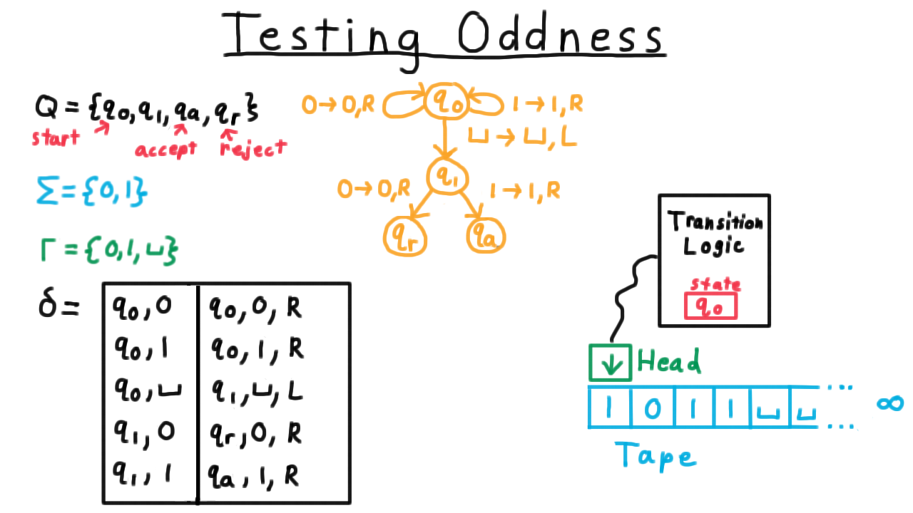
One convenient way represent the transition function, by the way, is with a state diagram, similar to what is often used for finite automata for those familiar with that model of computation. Each state gets its own vertex in a multigraph and every row of the transition table is represented as an edge. The edge gets labeled with remaining information besides the two states, that is the symbol that is read, the one that is written and the direction in which the head is moved.
See if you can trace through the operation of the Turing machine for the input shown. If you are unsure, watch the video.
Configuration Sequences - (Udacity, Youtube)
Recall that a Turing machine always starts in the initial state and with the head at the first position on the tape. As it computes, it’s internal state, the tape contents, and the position of the head will change, but everything else will stay the same. We call this triple of state, tape content, and head position a configuration, and any given computation can be thought of as a sequence of configurations. It starts with the initial state, the input string and with the head position on the first location, and it proceeds from there.
Now, it isn’t very practical always draw a picture like this one every time that we want to refer to the configuration of a Turing machine, so we develop some notation that captures the idea.

We’ll do the same computation again, but this time we’ll write down the configuration using this notation. We write the start configuration as \(q_0\)1011. The part to the left of the state represents the contents of the tape to the left of the head. It’s just the empty string in this case. Then we have the state of the machine and then the rest of the tape contents.
After the first step, 1 is to the left of the head, we are state \(q_0\) still and ‘1’ is the string to the right. In the next, configuration ‘10’ is to the left, we are still in state \(q_0\) and ‘11’ to right, and so on and so forth.
This notation is a little awkward, but it’s convenient for typesettings. It’s also very much in the spirit of Turing machines, where all structured data must ultimately be represented as strings. If a Turing machine can handle working with data like this, then so can we.
At a slightly higher level, a whole sequence of configurations like this captures everything that a Turing machine did on a particular input, and so we will sometimes call such a sequence a computation. And actually, this representation of a computation will be central as when we discuss the Cook-Levin theorem in the section on complexity.
The Value of Practice - (Udacity, Youtube)
Next, we are going get some practice tracing though Turing machine computations and programming Turing machines. The point of these exercises is not, so that you can put on your resume that you are good at programming Turing machines. And if someone asks you in an interview to write a program to test whether an input number is prime, I wouldn’t recommend trying to draw a Turing machine state diagram. Somehow, I doubt that will land you the job.
Rather, the point is to help you convince yourself that Turing machines can do everything that we mean by computation, and if you really had to, you could program a Turing machine to do anything that your could write a procedure to do in your favorite programming language. There are two ways to convince yourself of this. One is to just practice so that you build up enough of a facility with programming them – that is to say, it becomes easy enough for you– so that it just seems intuitive that you could do anything. Another way is to show that a Turing machine can simulate the action of models that are closer to real-world computers like the Random Access Model. We’ll do that in a later lesson. But, to be able to understand these simulation arguments, you need a pretty good facility with how Turing machines work anyway, so make the most of these examples and exercises.
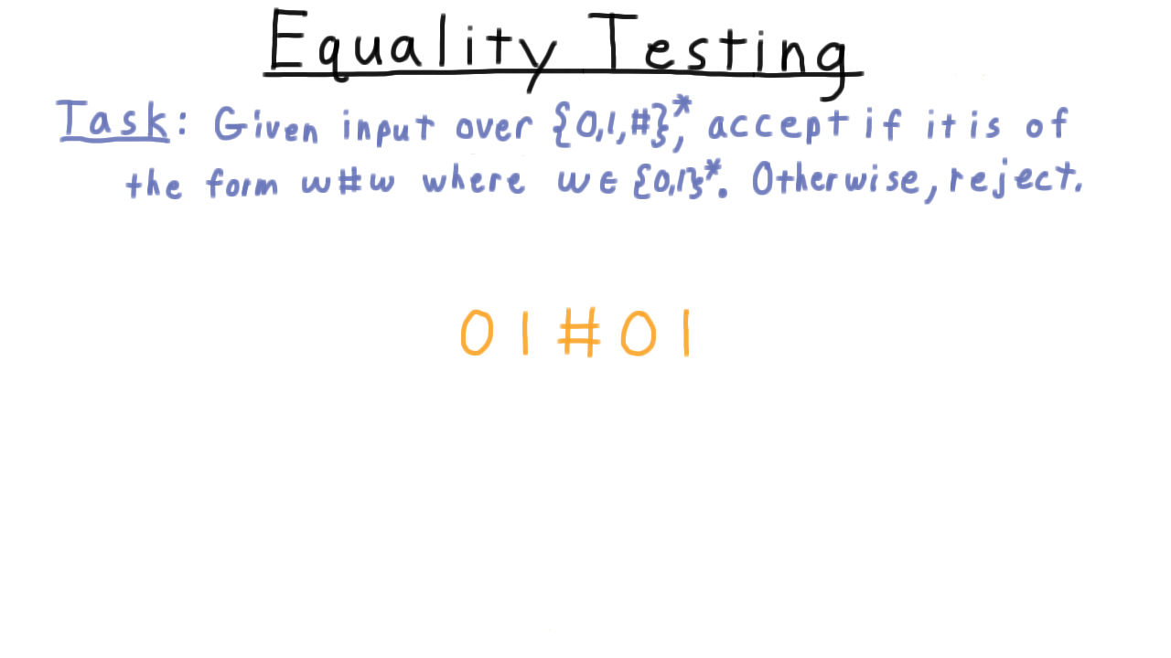
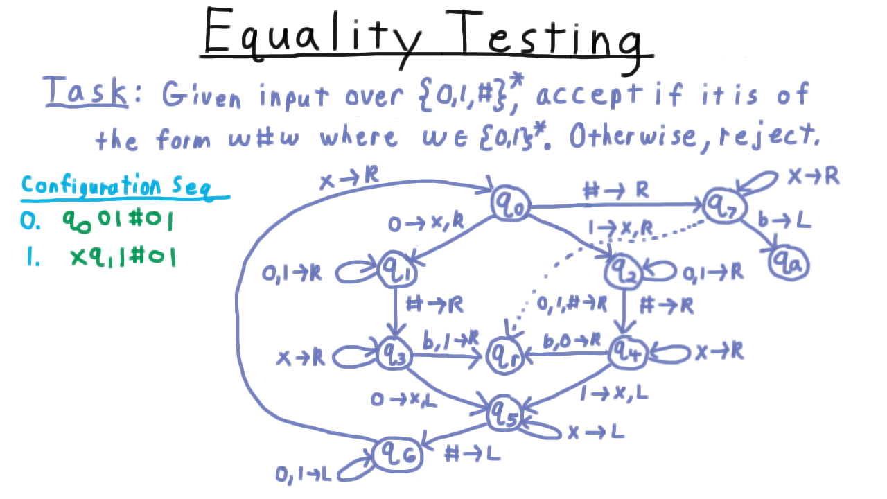
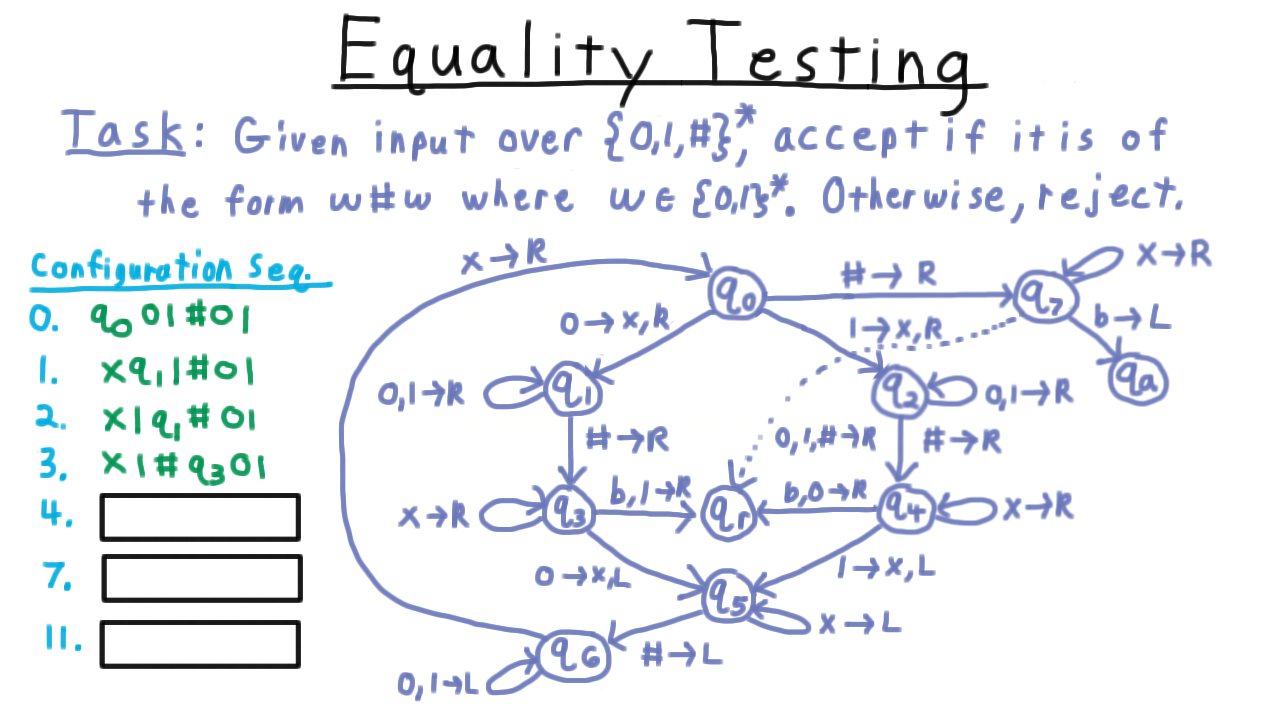
Equality Testing - (Udacity, Youtube)
To illustrate some of the key challenges in computing with Turing machines and how to overcome them, we’ll examine this task here, where we are given an input string, and want to tell if it is of the form w#w, where w is a binary string. In other words, we want to test whether the string to the left of the first hash is the same as the string to the right of it.
(Watch the video for an illustration on this example.)
As Turing machines go this is a pretty simple program, but as you can see here the state diagram gets a little messy. Like the Sisper textbook, I’ve used a little shorthand here in the diagram. When two symbols appear to the left of the arrow, I mean to either one of those. It’s easier than writing out a whole other edge. Also, sometimes, I will only give a direction on the right. Interpret that to mean that the tape should be left alone.
(Watch the video for an illustration of the state transitions in the diagram.)
Configuration Exercise - (Udacity)
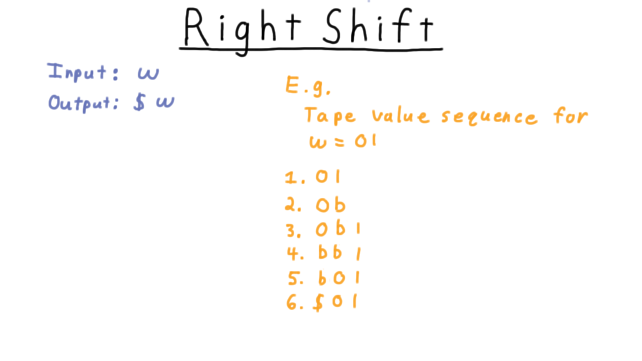
Right Shift - (Udacity)
Now, I want you to actually build a Turing machine. The goal is to right-shift the input and place a dollar sign symbol in front of the input and accept. Unlike our previous examples, accept vs. reject isn’t important here. This is more like a subroutine within a larger Turing machine that you might want to build, though you could think about it as a Turing machine that computes a function from all strings over the input alphabet to string over the tape alphabet, if you like.
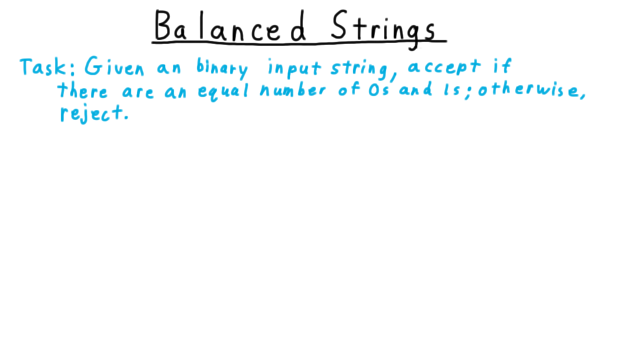
Balanced Strings - (Udacity)
Language Deciders - (Udacity, Youtube)
If you completed all those exercises, then you are well on your way towards understanding how Turing machines compute, and hopefully, also are ready to be convinced that they can compute as well as any other possible machine.
Before we move onto that argument, however, there is some terminology about Turing machines and the languages that they accept and reject those that they might loop on that we should set straight. Some of the terms may seem very similar, but the distinctions are important ones and we will use them freely throughout the rest of the course, so pay close attention. First we define what it means for a machine to decide a language.
A Turing machine decides a language L if and only if accepts every x in L and rejects every x not in L.

For example, the Turing machine we just described decided the language L consisting of strings of the form w#w, where w is a binary string. We might also say the Turing machine computed the function that is one if x is in L and 0 otherwise. Or even just that the Turing machine computed L.
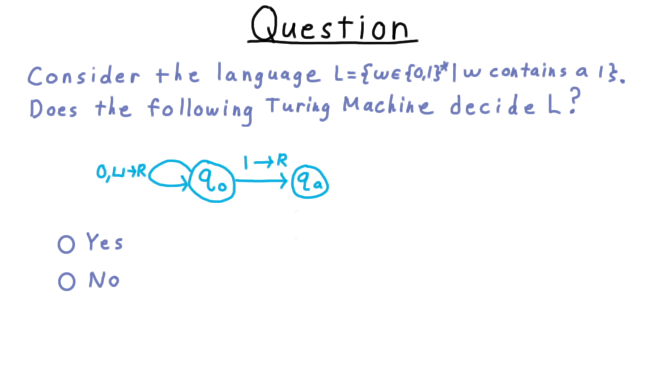
Contains a One - (Udacity)
Now for a question that is a little tricky. Consider the language that consists of all binary strings that contain a symbol 1. Does this Turing machine decide L?
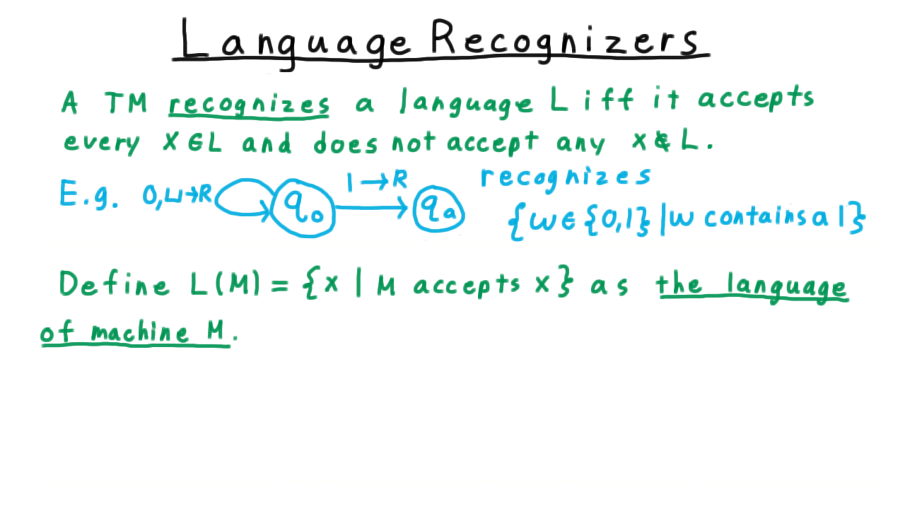
Language Recognizers - (Udacity, Youtube)
The possibility of Turing machines looping forever leads us to define the notion of a language recognizer.
We say that a Turing machine recognizes a language L if and only if it accepts every string in the language and does not accept every string not in the language. Thus, we can say that the Turing machine from the quiz does indeed recognize the language consisting of strings that contain a 1. It accepts those containing 1 and it doesn’t accept the others; it loops on them.

Contrast this definition with what it takes for a Turing machine to decide a language. Then it needs not only to accept everything in the language but it must reject everything else. It can’t loop like this Turing machine.
If we wanted to build a decider for this language we would need to modify the Turing machine so that it detects the end of the string and move into the reject state.
At this point, it also makes sense to define the language of a machine, which is just the language that the machine recognizes. After all, every machine recognizes some language, even if it is the empty one.
Formally, we define \(L(M)\) to be the set of strings accepted by \(M\), and we call this the language of the machine \(M\).
Conclusion - (Udacity, Youtube)
In this lesson, we examined the workings of Turing machines, and if you completed all the exercises, you should have a strong sense of how to use them to compute functions and decide languages. We’ve also seen how unlike some simpler models of computation, Turing machines don’t necessarily halt on all inputs. This forced us to distinguish between language deciders and language recognizers. Eventually, we will see how this problem of halting or not halting will be the key to understanding the limits of computation.
We’ve shown Turing machines can test equality of strings, not something that could be computed by simpler models like finite or push-down automaton that you might have seen in your undergraduate courses. But equality is a rather simple problem–can Turing machines solve the complex tasks we have our computer do. Can a Turing machines do your taxes or play a great game of chess? Next lesson, we’ll see that Turing machines can indeed solve any problem that our computers can solve and truly do capture the idea of computation.