Computability, Complexity, and Algorithms

Charles Brubaker and Lance Fortnow

Randomized Algorithms - (Udacity)

Introduction - (Udacity, Youtube)

In this lesson we are going to introduce a new element to our algorithms: randomization. In a full course on complexity or one on randomized algorithms, we might go back to the definition of Turing machines, include randomness in the model, and then argue that other models are equivalent. Here we are just going to assume that the standard built-in procedures available in most programming language work. Of course, in reality, these only produce pseudorandom numbers, but for the purpose of studying algorithms we assume that they produce truly random ones.

The lesson will use a few simple randomized algorithms to help motivate probability theory, and then use the basic theorems to characterize the behavior of a few slightly more sophisticated algorithms. Some ideas that come up include Independence, Expectation, Monte Carlo vs. Las Vegas algorithms, Derandomization, and in the end we’ll tie our study of algorithms back to complexity with a brief discussion of Probabilistically Checkable Proofs.

Verifying Polynomial Identities - (Udacity, Youtube)

Our first randomized algorithm will one that verifies polynomial identities. Suppose that you are working at company that is building a numerical package for some parallel or distributed system. A colleague claims that he has come up with some clever algorithm for expanding polynomial expressions into their coefficient form.
His algorithm takes in some polynomial expression and outputs a supposedly equivalent expression in coefficient form, but you are a little skeptical that his algorithm works for the large instances that he claims it works on. You decide that you want to write a test. That is to say that you want to verify that the polynomial represented by the input expression \(A\), is equivalent to the one represented by the output \(B.\)

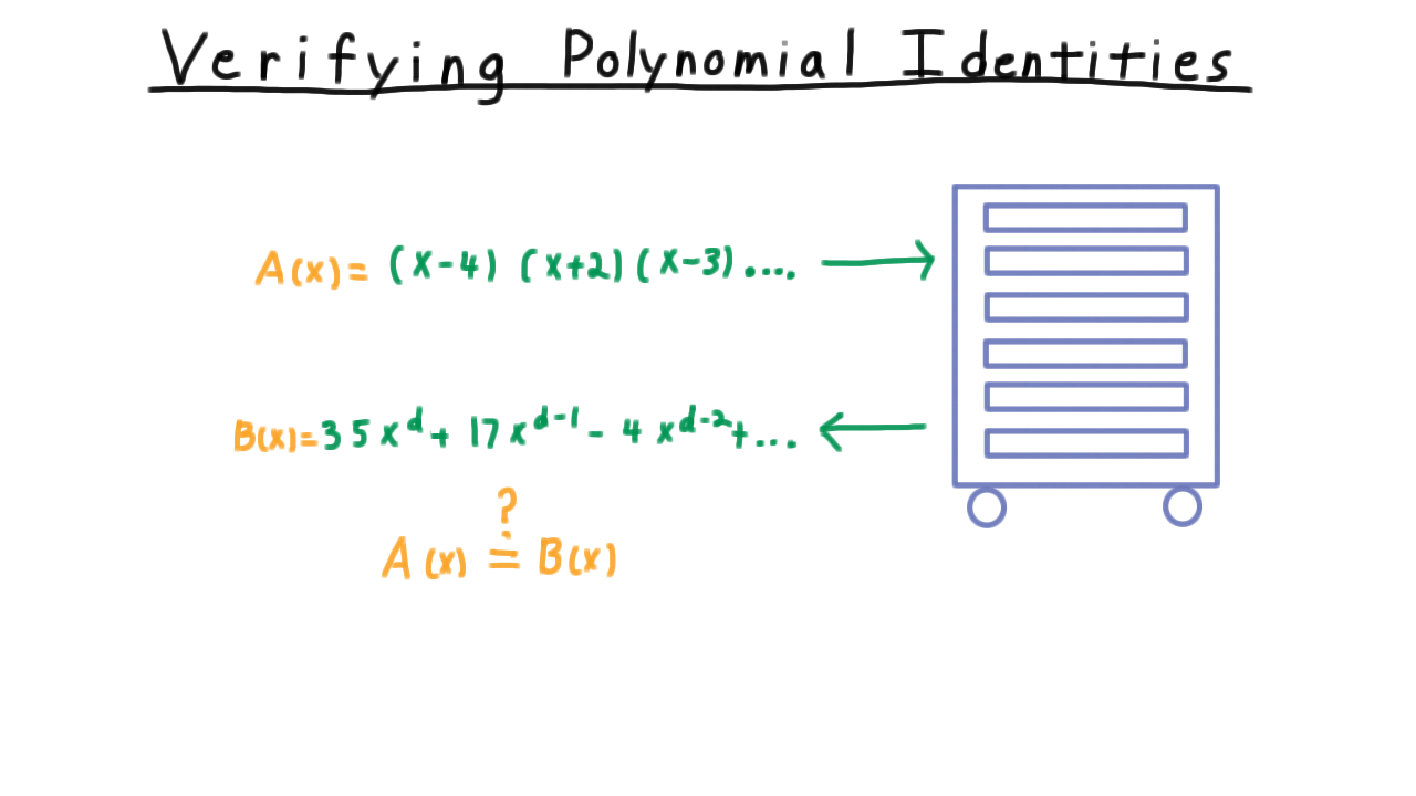
Being slightly more general, we can state the problem like this. Given representations of polynomials \(A\) and \(B\) having degree \(d,\) decide whether they represent the same polynomial. Note that we are being totally agnostic about how \(A\) and \(B\) are represented. We are just assured that \(A\) and \(B\) are indeed polynomials, and we have a way of evaluating them. Well, here is a fantastically simple algorithm for deciding whether these two polynomials are equal.

1. Pick a random integer in the range \([1, 100d].\)
2. Evaluate the polynomials at this points.
3. Say that the polynomials are equal if they are equal at this point.

Why does this work? Well, the so-called Fundamental Theorem of Algebra says that any non-zero polynomial can have at most d roots.

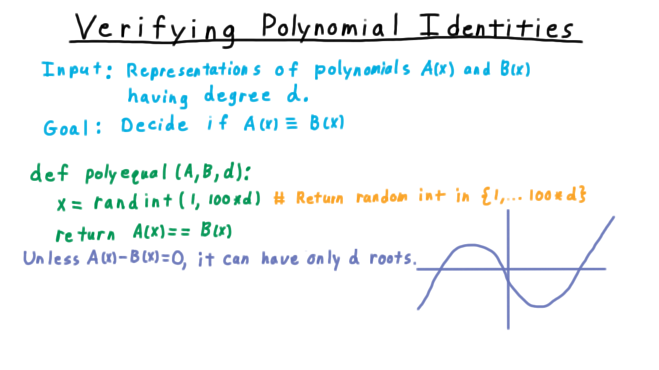
So if \(A\) and \(B\) are different, the bad case is that it has \(d\) roots and what’s worse that all of them are integers in this range \([1,100d]\). Even so, the chance that the algorithm picks on of these is still only \(1/100.\) So if the polynomials are the same, we will always say so, but if they are different, then we will say they are the same is a chance 1 in 100. This is pretty effective, and if it is found that \(A\) is not equal to \(B\) in some case, your algorithm is so simple that there can’t be much dispute o over which piece of code is incorrect.

Discrete Probability Spaces - (Udacity, Youtube)

In the analysis of the algorithm for polynomial identity verification, I avoided the word probability because we haven’t defined what it means yet. We’ll do that now and use the algorithm to illustrate the meaning of the abstract mathematical turns.

A discrete probability space consists of a sample space Omega that is finite or countably infinite. This represents the set of possible outcomes from whatever random process we are modeling. In the case of the previous algorithm, this is the value of x that is chosen.

Second, a discrete probability space has a probability function with these properties. It must be defined from the set of subsets of the sample space to the reals. Typically, we call a subset of the sample space an event \(E.\) For every event, the probability must be at least 0 and at most 1. The probability of the whole sample space must be 1. And for any pairwise disjoint collection of events the probability of the union of the events must be the sum of the probabilities.

To illustrate this idea with the polyequal example, let’s define the events \(F_i\) to be the set consisting of the single element \(i,\) i.e. \(F_i = \{i\}.\) This corresponds to \(i\) being chosen as the value at which we test the polynomials. And we define the probability of the event \(F_i\) as \(\Pr(F_i) = 1/100d.\) Now, these \(F_i\) aren’t the only possible events. They are just the single elements sets of the probability space. We need to define our function over all subsets. But actually, we have done so implicitly already because of property 2c above. For any subset \(S\) of the sample space, we have that the subset is the union of the individual events \(F_i.\) These are disjoint, so the probability of the union is the sum of the probabilities, and so the result is the size of the set divided by the size of the sample space, as we would expect. That is to say
\[ \Pr(S) = \Pr(\cup_{i \in S} F_i)= \sum_{i \in S} \Pr(F_i) = \frac{|S|}{|\Omega|}\]

Let’s confirm that this function meets all of the requirements of the definition. Property 2c holds because the size of a disjoint union is the sum of the sizes of the individual sets. We see from the ratio \(\Pr(S) = |S|/|\Omega|\) that the probability of the whole sample space is \(1.\) And the probability of any event is between 0 and 1. So this example here is, in fact a discrete probability space.

By the way, this example probability function is called uniform, because the probability of every single element event–that is to say the \(F_i\) here are the same. Not all probability functions are like that.

Bounding Probabilities - (Udacity)

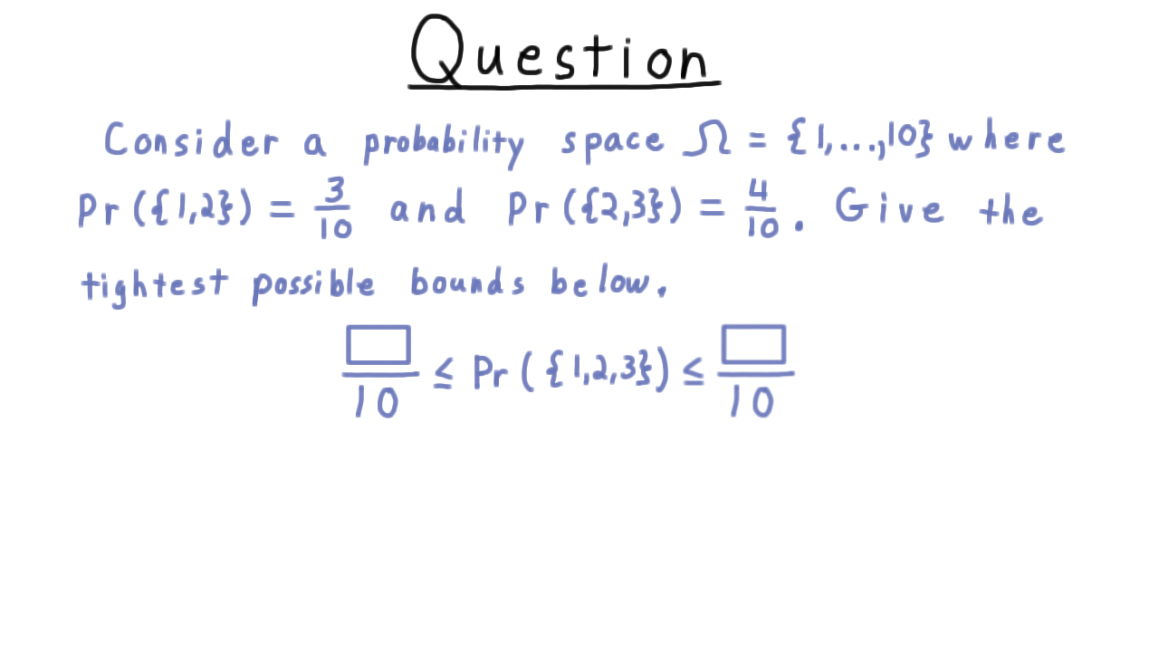
Here is a quick exercise on probability spaces. Consider one where the sample space are the integers 1 to 10, where the probability of 1 or 2 is 3/10 and the probability of 2 or 3 is 4/10. Based on this information, I want you to give the tightest bound you can on the probability of 1, 2, or 3.

Repeated Trials - (Udacity, Youtube)

Let’s return to our polynomial identity verification algorithm and see if we can improve it. So far, we’ve seen how if the two polynomials are equal, the algorithm will always say so. But if the polynomials are different, there is up to a \(1/100\) probability that the algorithm will say that they are equal anyway. Maybe this isn’t good enough. We want to do better. One idea is just to change out the number \(100\) for a larger number. This works, but on a real computer we might start to run into range problems. We don’t want our algorithm to strain the difference between the theoretical models and practice.

Another solution is repeated trials. Instead of just testing for equality at one point, we’ll do it at several random ones. Such an algorithm might look like this.

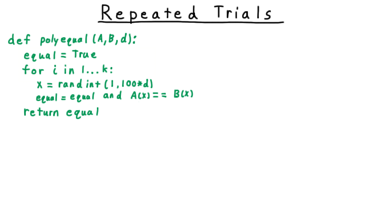
We start out by assuming that the two polynomials are equal. Then we try different values for \(x,\) and if we ever find a value for which the two polynomials are not equal then we know that they aren’t. Note that we could terminate as soon as a difference is found, but this version of the algorithm makes the analysis a little more clear.

For simplicity, we’ll make this \(k\) equal to \(2\) so that we can visualize the sample space with a 2D grid like so.

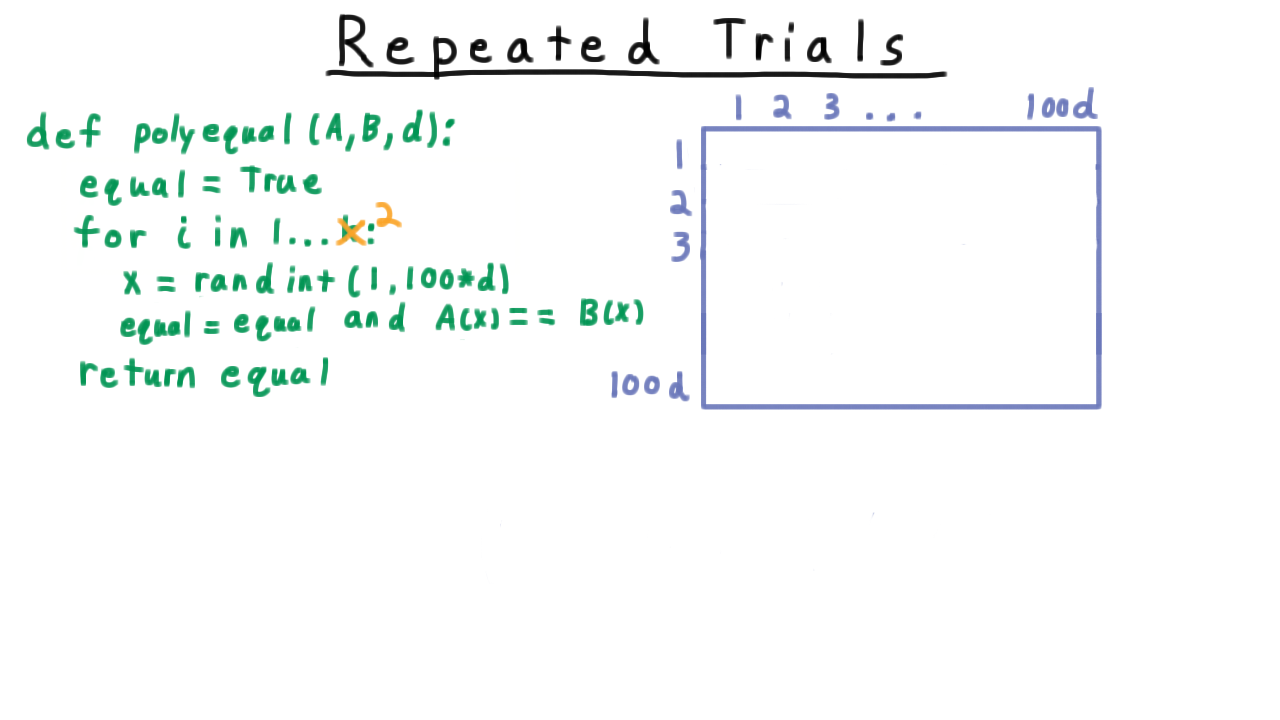
The row corresponds to the value of \(x\) in the first iteration, the column to the value of \(x\) in the second iteration. Now, the size of the sample space is \((100d)^2\) and since there are \(d^2\) pairs of roots for the difference between \(A\) and \(B,\) at most \(d^2\) of these possibilities make the algorithm fail.We’ll let \(F\) be the event that the algorithm fails on unequal polynomials. That is, the probability that \(A(x) = B(x)\) for both chosen \(x.\) By symmetry, we can argue that all elements of the sample space should have equal probability, so the probability of the algorithm failing on two unequal polynomials \[ \Pr(F) \leq \frac{d^2}{(100d)^2} = \frac{1}{100^2}.\] That’s 1/100th of the probability one for just one trial.

We can also make the argument by following the actual process of the algorithm more closely. We let \(E_1\) be the even that the polynomials are equal at \(x\) in the first iteration. In terms of our grid, this is the subset of the sample space as subset of the rows.

As we argued before, this probability is \(\Pr(E_1) \leq \frac{1}{100}\).

Similarly, we let \(E_2\) be the event that the polynomials are equal at \(x\) in the second iteration. In the grid, this event corresponds to a certain subset of the columns. Again, these red columns take up at most 1/100th of the whole probability mass.

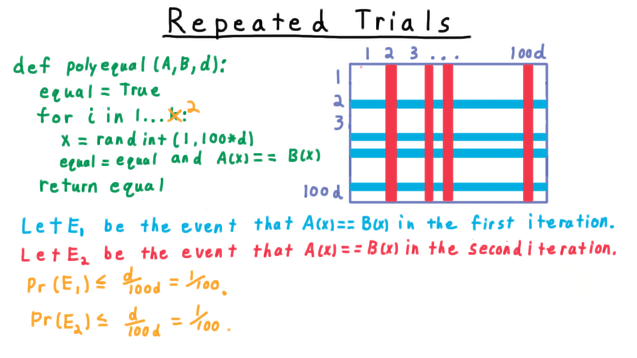
We are interested in the probability of both \(E_1\) and \(E_2\) happening–i.e. the intersection of these two events, represented as the black region in our grid.

What fraction of the probability mass does it take up? Notice that in order for a sample to fall into the black region, the first iteration must restrict us to the the blue region. The probability of this happening is is just the probability of \(E_1.\) Then from within the blue region, we ask what fraction of the probability mass does of \(E_2\) take up? Well, that’s just \(\Pr(E_1 \cap E_2)/\Pr(E_1),\) and we want to multiply this quantity with \(Pr(E_1)\) to get the result. This sort of ratio is common enough that it gets its own name and notation. We notate it like so, \[\Pr(E_2|E_1) \equiv \frac{\Pr(E_1\cap E_2)}{\Pr(E_1)},\]

and read this as the probability of \(E_2\) given \(E_1.\) This is called a conditional probability. The interpretation is that it gives the probability of \(E_2\) happening, given that \(E_1\) has already happened.

More specifically for our polynomial verification, the probability that the second iteration will pick a value where the polynomials are equal given that the first one did. Well, of course, this is that same probability as \(E_2\) happening, regardless of what happened with in the first iteration, so this is just the probability of \(E_2\). This is a condition known as independence, and it corresponds to our intuitive notion of one event not depending on another.

Substituting in these values we find that that this approach gives the same result as the other.

\[Pr(E_1 \cap E_2) = \Pr(E_1) \Pr(E_2 | E_1) = \Pr(E_1) \Pr(E_2) = \frac{1}{100^2}.\]

Independence and Conditional Probability - (Udacity, Youtube)

We just used the ideas of conditional probability and independence in the context of our polynomial verification algorithm. Now, let’s discuss these ideas in general. We define the conditional probability that an event \(E\) occurs given that event \(F\) occurs as the ratio between the probability than both \(E\) and \(F\) occur divided by the probability that \(F\) occurs.

We can visualize this quantity using a traditional Venn diagram. We draw the whole sample space as a large rectangle, and within here we draw the set F like so.

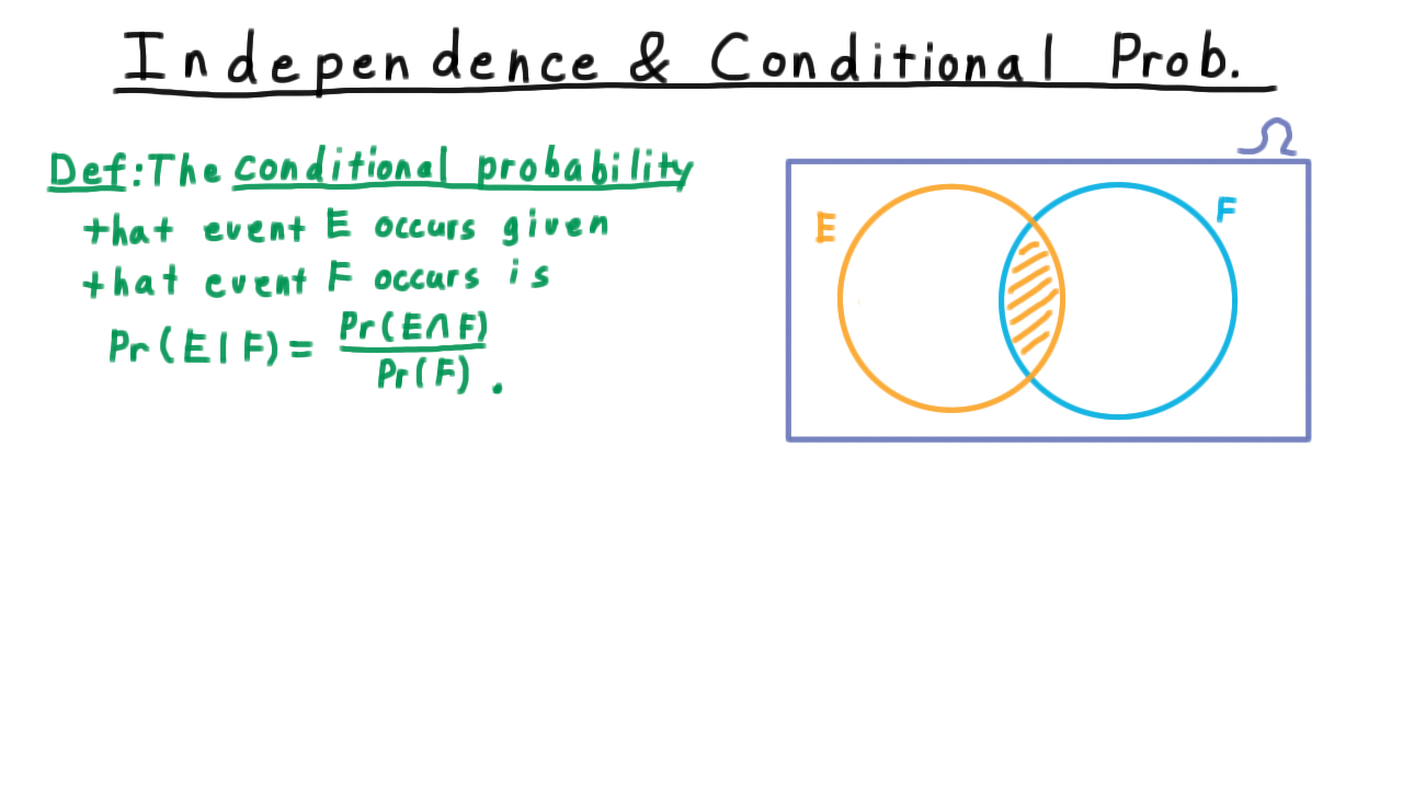
When we talk about conditional probability of \(E\) given \(F,\) we are restricting ourself to the set \(F\) within the sample space. Thus, only the portion of \(E\) that is also in \(F\) is important to us. To make this a proper probability we have to renormalize by dividing by the probability of \(F.\) That way, the probability of \(E\) given \(F\) and the probability of not \(E\) given \(F\) sum up to 1.

\[\Pr(E|F) + \Pr(\overline{E}|F) = \frac{\Pr(E \cap F)}{\Pr(F)} + \frac{\Pr(\overline{E} \cap F)}{\Pr(F)} = \frac{\Pr(F)}{\Pr(F)} = 1\]

An interesting situation is where the probability of an event \(E\) given \(F\) is the same as the probability when \(F\) isn’t given.
\[\Pr(E|F) = \Pr(E)\]
This implies that \(E\) and \(F\) are independent. One doesn’t depend on the other. Formally, we say

Two events \(E\) and \(F\) are independent if \[\Pr(E \cap F) = \Pr(E)\Pr(F)\]

Note that this is a slightly more general statement than saying \(\Pr(E|F) = \Pr(E).\) The quantity \(\Pr(E|F)\) isn’t defined if \(\Pr(F) = 0.\)

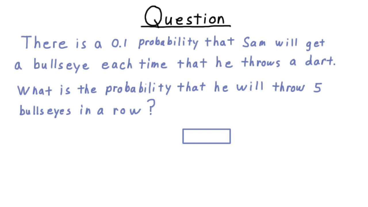
Bullseyes - (Udacity)

Here is a quick question on independence. Suppose that there is a 0.1 probability that Sam will get a bulleyes each time that he throws a dart. What is the probability that he gets 5 bullseyes in a row?

Monte Carlo and Las Vegas - (Udacity, Youtube)

Let’s go back to our polynomial verification algorithm with repeated trials and review its behavior.

If the two input polynomials are equal, then the probability that the algorithm says so is 1. On the other hand, if the polynomials are different, there is a chance that the algorithm we get the answer wrong, but this happens only with probability \(100^{-k}\) where \(k\) is the number of trials that we did. We just need to extend the argument we made before for \(k=2\) to general \(k.\)

The fact that our algorithm might sometimes return an incorrect answer makes it what computer scientists call a Monte Carlo algorithm. And because it makes a mistake only when the polynomials differ, it is called one-sided Monte Carlo algorithm. This idea can be extended to arbritrary languages. Here strings in the language represent equal polynomials. This algorithm only makes mistakes on strings not in the language. Of course, its possible for the situation to be reversed so that the algorithm makes mistakes on string in the language. This is another kind of one sided Monte Carlo algorithm. I should say that there are also two-sided Monte-Carlo algorithm, where both errors are possible, but regardless of what input is given the answer is more likely to be correct than not.

Suppose, however, that any possibility of error is intolerable. Can we still use randomization? Well, yes we can. Instead of picking a new point uniformly at random from the \(100d\) possible choices, we can pick one from the choices that we haven’t picked before. This is known as sampling without replacement, since we don’t replace the same we took back in the pool before choosing again. There are only d possible roots, by the time we’ve pick the \((d+1)\)th point, so we must have picked one of the non-roots.

This algorithm still uses randomization, but nevertheless it always gives a correct answer. If the polynomials are equal, the probability that the algorithms says so is 1. If they are unequal, the probability that it says they are equal is 0.
The fact that this algorithm never returns an incorrect answer makes it a Las Vegas algorithm. The randomization can effect the running time, but not the correctness. If the polynomials are equal, the algorithm definitely takes \(d+1\) iterations, but when they are unequal, it gets a little more complicated.

Let \(E_i\) be the event that \(A\) and \(B\) are equal at the ith element of the order array chosen randomly by the algorithm above. Then, we characterize the probability that the algorithm takes at least \(k\) steps as \(\cap_{i=0}^{k-1} E_i.\) Note, however, that these events are no longer independent. If \(A\) and \(B\) are equal at the first element of the list order, then that’s one fewer root that could have been chosen to be the second element. So how do we go about calculating this probability?

Sampling without Replacement - (Udacity)

Let’s make this calculation for a concrete example an exercise. Suppose that the difference \(A-B\) is a polynomial of degree 7 with 7 roots in the set of integers 1 through 700. An algorithm samples 3 of these numbers uniformly without replacement. Give an expression for the probability that all of these points are roots of the difference \(A-B.\)

Returning to the Las Vegas version of our polynomial identity verifier, we can write the probability that we don’t detect a difference in k iterations as the product

\[\Pr(\cap_{i=0}^{k-1}) = \Pr(E_1)\Pr(E_2|E_1) \ldots \Pr(E_{k-1}|E_1 \cap E_2 \cap \ldots \cap E_{k-2}) = \prod_{i=0}^{k-1} \frac{d-k}{100d-k} \leq \frac{1}{100^k}.\]

With a little more work, we can get a tighter bound that this, but for our purpose this simple bound works. Note that even though the probabilities for the LasVegas and Monte Carlo algorithms are the same, the meanings are different. In the Monte Carlo algorithm, our analysis captured the probability of the the algorithm returning a correct answer. In the Las Vegas algorithm, our analysis something about the running time for an algorithm that will always produce the correct answer.

Random Variables - (Udacity, Youtube)

So far, all the probabilistic objects we’ve discussed have been events–things that either happen or don’t happen. As we go further in our analysis, however, it will be convenient to talk about other random quantities: what is value of a random die roll? or how many times did we have to repeat that procedure before we got an acceptable outcome? For this, we introduce the idea of a random variable.

A random variable on a sample space \(\Omega\) is a function \(X:\Omega \rightarrow \mathbb{R}\)

For example, let \(X\) be the sum of two die throws. Then, the sample space is \(\Omega = \{1,\ldots,6\}\times \{1,\ldots,6\}\), and the random variable \(X\) is the function that just adds those two numbers together,
\[X((i,j)) = i+j.\]

We use the notation \(X = a\) where \(a\) is some constant to indicate the event that \(X\) is equal to \(a.\) Thus, it is the set of elements for the sample space for which the function X is equal to A. In our example,
\[ (X=3) = \{(1,2),(2,1)\}.\]

Expectation - (Udacity, Youtube)

Having defined a random variable, it now makes to talk about a random variable’s average or expected value. Formally,

The expectation of a random variable \(X\) is \[ E[X] = \sum_{v \in X(\Omega)} v \Pr(X=v),\] where \(X(\Omega)\) is the image of \(X.\)

A can be seen from the formula, the expectation is a weighted average of all the values that the variable could take on. For example, let the random variable \(X\) be number of heads in 3 fair coin tosses. Then, according to this definition, the expectation would be:

• \(0 \cdot \frac{1}{8}\) for getting no heads.


• \(1 \cdot \frac{3}{8}\) for getting 1 head, as there are three possible tosses that could have come up heads.


• \(2 \cdot \frac{3}{8}\) for getting 2 heads, as there are three possible tosses that could have come up tails to give us two heads.


• \(3 \cdot \frac{1}{8}\) for getting 3 heads.

Adding these all up we get \(12/8 = 3/2.\) Now, if I asked you casually, how many heads will there be in three coins tosses on average, you probably would have said\( 3/2\) rather quickly and without doing all this calculation. Each toss should get you \(1/2\) a head, so with \(3\) your should get \(3\) halves, you might have reasoned.

In terms of our notation, we can express the argument like this. We let \(X_i\) be 1 if the \(i\)th fair coin toss is heads and 0 otherwise. Then we say that the average number of heads in three tosses is
\[E[X_1 + X_2 + X_3] = E[X_1] + E[X_2] + E[X_3] = \frac{3}{2}.\]

The key step in the proof is the first equality here, which says that the expectation of the sum is the sum of the expectations. This is called the linearity of expectation, and as we will see, this turns out to be a very powerful idea.

In general,

For any two random variables \(X\) and \(Y\) and any constant \(a\), the following hold \[ E[X + Y] = E[X] + E[Y] \] and \[E[aX] = aE[X]\].

The expectation of the sum is the sum of the expectations, and we can just factor out constant factors from expectations. Remember this theorem.

Counting Cycles in a Permutation - (Udacity)

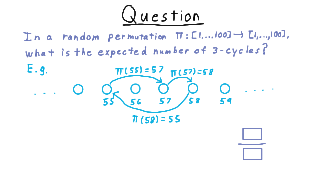
Here is an exercise that will help illustrate the power of the linearity of expectations. In a random permutation over 100 elements, what is the expected number of 3-cycles?

We can think about the permutation as defining a directed graph over 100 vertices, where every vertex has exactly one outgoing and one incoming edge, which are defined by the permutation. Thus, if \(\pi(55)=57,\) we would draw this edge here, if \(\pi(57)=58,\) we draw this edge here, and if \(\pi(58) = 55,\) we would draw this edge here. Together, these form 3 cycle.

Use the linearity of expectation and write down the expected number of 3-cycles as a ratio here.

Quicksort - (Udacity, Youtube)

At this point, we’ve covered the basics of probability theory, so we’ll be able to turn our focus on the algorithms themselves and their analysis. Up first is the classic randomized quicksort algorithm.

I case you don’t recall randomized quicksort from a previous algorithms course, here is the pseudocode.

To keep things simple, we’ll assume that the elements to be sorted are distinct. This is a recursive algorithm, with the base case being a list of 0 or 1 elements, where the list can simply be returned. For longer lists, we choose a pivot uniformly at random from the elements of the list, and then split the list into two pieces: one with those element less than the pivot and one with those elements larger than the pivot. We then recursively sort these shorter lists and then join them back together once they are sorted.

The efficiency of the algorithm depends greatly on the choices of the pivots. We can visualize a run of the algorithm by drawing out the recursion tree. I’ll write out the list is sorted order so that we can better see what is going on, though the algorithm itself will likely have these elements in some unsorted order.

The ideal choice of pivot is always the middle value in the list. This splits the list into two equal-size sublists. One consisting of the larger elements, the other of the smaller elements. Then in the recursive calls, we split these lists into two pieces, until we get down to the base case.

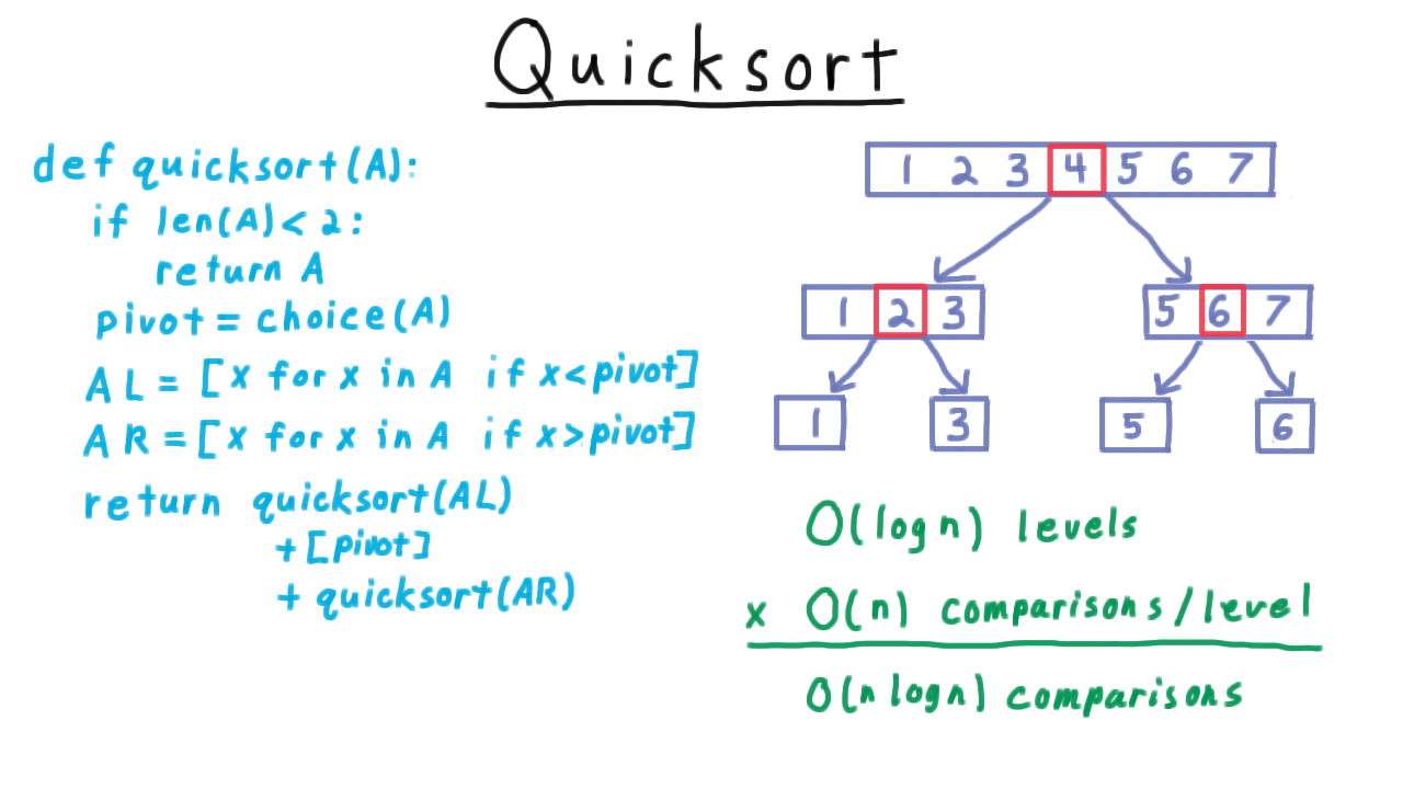
Because the size get cut in half with each call, there are only \(\log n\) levels to the tree. Every element gets compared with a pivot, so there are \(O(n)\) comparisons at each level, for a total of \(O(n \log n)\) comparisons overall. That’s if we are lucky and pick the middle element for the pivot every time.

How about if we are unlucky? Suppose we pick the largest element in every iteration.

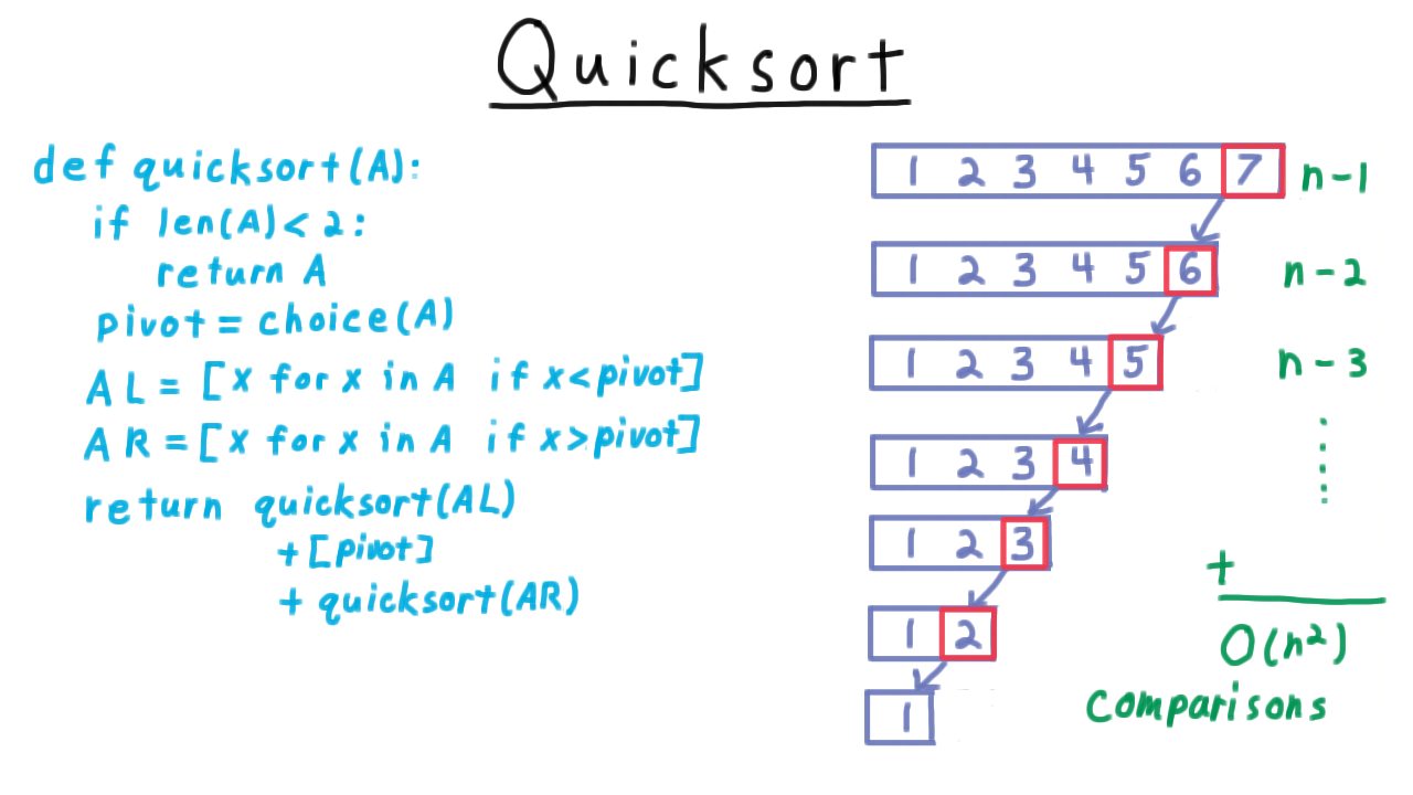
Then the size of the list only decreased by one in every iteration, so there are n levels. The first level require \(n-1\) comparison, the second \(n-2\) and so forth, so that the total number of comparisons is an arithmetic sequence and therefore is \(O(n^2).\) This is as bad as a naive algorithm like insertion sort. The natural question to ask then, how does quicksort behave on average? Is it like the best case where the pivot is chosen in the middle, the worst case that we have here, or somewhere in-between?

Analysis of Quicksort - (Udacity, Youtube)

Now, we’ll analyze the average case performance of quicksort and show that it is \(O(n \log n)\), just like the optimum case. Suppose that the randomized quicksort algorithm is used to sort a list consisting of elements \(a_1 < a_2 < \ldots < a_n \) all of which are distinct.

We’ll let \(E_{ijk}\) be the event that \(a_i,\) the ith largest element in the list, is separated from \(a_j,\) the jth largest element in the list, by the kth choice of a pivot. And, we’ll let \(X_{ij}\) be a variable that is 1 if the algorithm actually compares \(a_i\) with \(a_j\) and 0 otherwise. The sum of the \(X_{ij}\) will count the number of comparisons that the algorithm uses.

Claim: \[E [ \sum_{i < j} X_{ij}] = \frac{2}{j-i+1}\]

For the proof, observe that
\[ E[X_{ij}] = 1 \cdot \Pr(X_{ij} = 1) + 0 \cdot \Pr(X_{ij} = 0) = \Pr(X_{ij} = 1)\]
In fact, the expectation of all zero-one variables is just the probability that the variable is equal to one.

The element \(a_i\) has to be separated from \(a_j\) by some pivot in the algorithm, and they won’t be separated by two. Therefore, fixing \(i\) and \(j,\)the events \(E_{ijk}\) are disjoint, so
\[ \Pr(X_{ij} = 1) = \sum_k \Pr(X_{ij} = 1 \cap E_{ijk}).\]

This argument is known as the law of total probability.

Each non-zero term here can be written as a conditional expectation,
\[\sum_{k : \Pr(E_{ijk}) > 0} \Pr(X_{ij} = 1 \cap E_{ijk}) = \sum_{k : \Pr(E_{ijk}) > 0} \Pr(X_{ij} = 1| E_{ijk})\Pr(E_{ijk})\]
and it’s the conditional probability that will be easiest to reason about.

Given that \(a_i\) is going to be separated from \(a_j\), it must be that they haven’t been separated yet. So this list must include \(a_i, a_j,\) every element in-between possibly some more to the outside.

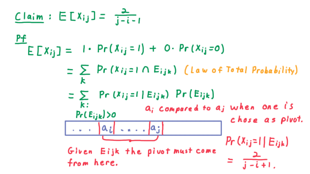
Given that the separation does occur, however, the pivot must be chosen in the range \([a_i,a_j].\) The element \(a_i\) will only be compared to \(a_j,\) however, if one of the two are chosen as the pivot. Therefore, given that the separation is going to occur, the probability that is will actually require a comparison is only \(2\) divided by the number of possible choices for the pivot \((j-i+1).\) Substituting, this value here will give us the answer.
\[\sum_{k : \Pr(E_{ijk}) > 0} \Pr(X_{ij} = 1| E_{ijk})\Pr(E_{ijk}) = \sum_{k : \Pr(E_{ijk}) > 0} \frac{2}{j-i+1} \Pr(E_{ijk}) = \frac{2}{j-i+1}.\]

With the claim established, we argue that by the linearity of expectation the expected number of total comparisons is just the sum of the expectations for
these \(X_{ij}\)s.
\[\sum_{i < j} E[X_{ij}] = \sum_{i < j} \frac{2}{j-i+1} \leq \sum_{i=1}^n \sum_{j=1}^n \frac{1}{j} = O(n \log n). \]

It’s possible to do some tighter analysis, but for our purposes is enough to use this loose bound, which becomes just the sum of n harmonic series. Summing \(1/j\) is rather like integrating \(1/x,\) so the inner sum becomes a \(\log\) and we get \(O(n \log n)\) in total.

Overall, then we can state our results as follows.

For any input of distinct elements quicksort with pivots chosen uniformly at random compares \(O(n \log n)\) elements in expectation.

The average case is on the same order as the worst case. This is comforting but by itself it is not necessarily a good guarantee of performance. It’s conceivable that the distribution of running times could be very spread out, so that it would be possible for the running time to be a little better than the guarantee or potentially much worse.

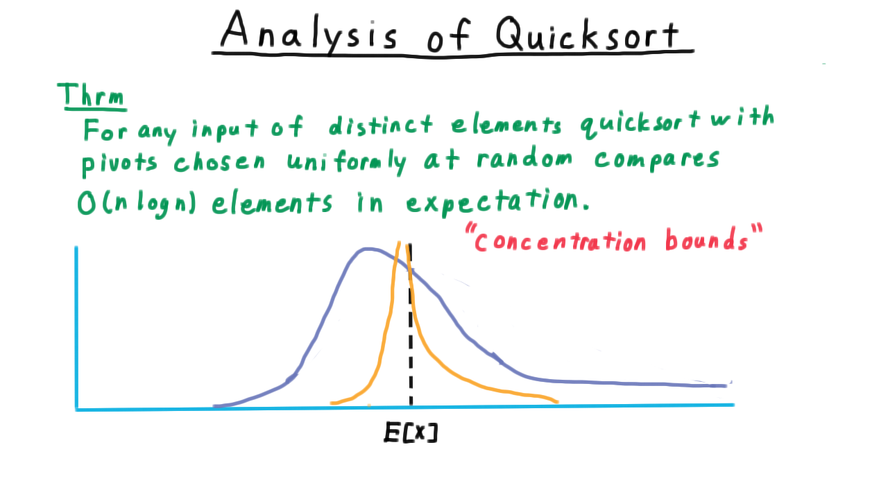
It turns out that this is not case. The running times are actually quite concentrated around the expectation, meaning the one is very unlikely to get running time much larger than the average. This sort of argument is called a concentration bound, and if you ever take a full course on randomized algorithms, a good portion will be devoted to these types of arguments.

A Minimum Cut Algorithm - (Udacity, Youtube)

Next, we consider a randomized algorithm for finding a minimum cut in a graph. Likely, this won’t be as familiar as quicksort. We are given a connected graph G, and the goal is to find a minimum sized set of edges whose removal from the graph causes the graph to have two connected components.

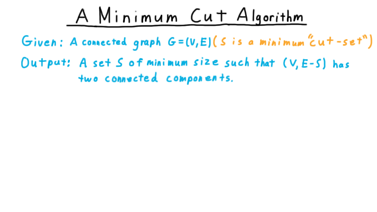
This set of edges \(S\) is called a minimum cut set. Note that this is a different problem from the minimum s-t cuts that we considered in the context of the maximum flow. There are no two particular vertices that we are trying to separate here–any two will do–, and all the edges have equal weight here. We can use a the minimum s-t cut algorithm to help solve this problem, but I think you will agree that this randomized algorithm is quite a bit simpler.

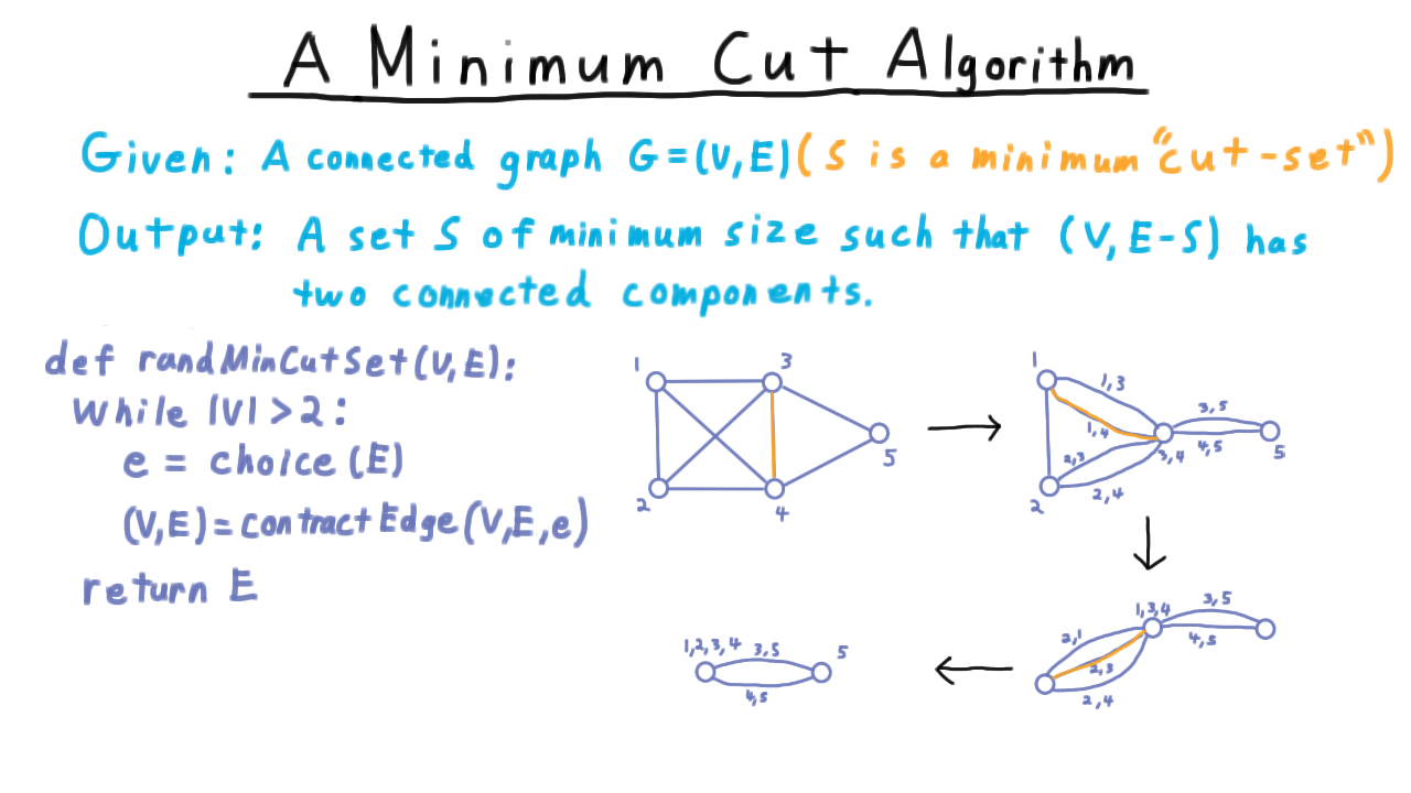
The algorithm operates by repeatedly contracting edges so as to join the two vertices together. Once there are only two vertices left, they define the partition. (See video for animated example.)

Now, this particular choice of edges led to a minimum a cut set, but not all such choices would have. How then should we pick an edge to contract?

It turns out that just picking a random one is a good idea. More often than not, this won’t yield a correct answer, but as we’ll see its will be often enough to be useful.

Analysis of Min Cut - (Udacity, Youtube)

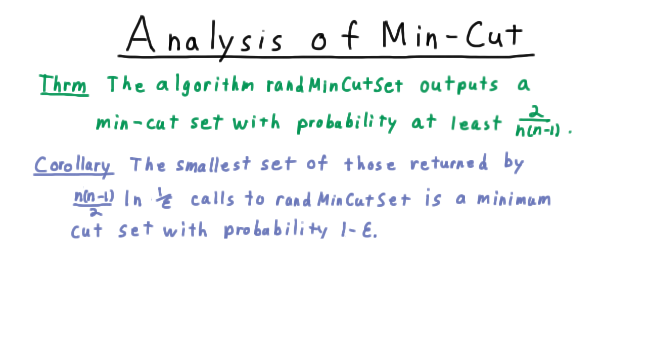
The algorithm just presented is known as “Karger’s Min-Cut Algorithm” and it turns out that

Karger’s minimum cut algorithm outputs a min-cut set with probability at least \(\frac{2}{n(n-1)}\).

Now at first, you might look at this result and ask “what good is that?” The algorithm doesn’t even promise to be right more often than not. The trick is that we can call the algorithm multiple times an just take this minimum of the result. If we do this \(n(n-1) \log (1/\epsilon)\) times then there is a \(1-\epsilon\) chance that we will have found a minimum cut set.

The proof for this corollary is that each call to the algoirthm is independent, so the probability that all of the calls fail is given by
\[ \left(1 - \frac{2}{n(n-1)}\right)^{\frac{n(n-1)}{2} \log (1/\epsilon)}.\]

In general \(1-x \leq e^{-x}\), so applying that inequality, we have that the n(n–1)/2 factors cancel in the exponent and we are left with

\[ \exp( - \log (1/\epsilon)) = \epsilon. \]

Thus, the probability that all the iterations fail is at most \(\epsilon,\) so the chance that at least one them succeeds is \(1-\epsilon.\) This bound here is extremely useful in analysis and is one that you should always have handy in your mental toolbox.

So if the theorem is true, we can boost it up into an effective algorithm just by repeating it, but why is the theorem true?

Consider a minimum cut set, and let \(E_i\) be the event that the edge chosen in iteration i of the algorithm in not in \(C.\) Note that there could be other minimum cut sets as well. For the analysis, however, we’ll just consider the probability of picking this particular one.

Returning the cut-set \(C\) means not picking an edge in \(C\) in each iteration, so it’s the intersection of all the events \(E_i,\) which we can turn into this product,
\[ \Pr(\cap_{i=1}^{n-2}) = \Pr( E_{n-2} | \cap_{i=1}^{n-3} E_i ) \ldots \Pr(E_2|E_1) \Pr(E_1)\]

as we’ve done before. We’re just conditioning the probability of avoiding \(C\) in the ith iteration given that we’ve avoid it in all previous ones.

We now make the claim

Claim: \[\Pr( E_{j+1} | \cap_{i=1}^{j} E_j ) \geq \frac{n-j-2}{n-j}. \]will be a little easier to analyze if we write as

We’ll warm-up just be considering, the probability of \(E_1\)–of avoiding the cut in the first iteration.

Letting the size of the cut be \(k,\) we have that every vertex must have degree at least \(k.\) Otherwise, the edges incident on the smaller degree vertex would be smaller cut set. This then implies that \(|E| \geq \frac{nk}{2}\)–every vertex must have degree at least \(k\) and summing up the degrees for every vertex counts every edge exactly twice. Therefore, the probability of avoiding the cut set \(C\) is
\[ \Pr(E_1) = 1 - \frac{|C|}{|E|} \leq 1 - \frac{k}{nk/2} = \frac{n-2}{n}\]
The more general argument will be similar.

Given that the first \(j\) edges chosen were not in \(C,\) then \(C\) is still a min cut-set. If not, then by taking those same edges in the original graph we would have a smaller cut-set than \(C.\) Note that throughout we count parallel edges.

Again, letting \(k\) be the size of \(C\), we have that there must be at least \(k(n-j)/2\) edges left. The \(n-j\) comes from the fact that there are only \(n-j\) vertices left after \(j\) iterations.
With the same argument as before, we have that the probability of avoiding \(C\) in the \(j+1\) iteration given that no edges in \(C\) have been chosen yet is
\[ \Pr(E_{j+1} | \cap_{i=1}^{j} E_i ) = 1 - \frac{|C|}{|E|} \geq 1 - \frac{k}{(n-j)k/2} = 1 - \frac{2}{n-j} = \frac{n-j-2}{n-j}.\]
as claimed.

Substituting, back into our equation here,

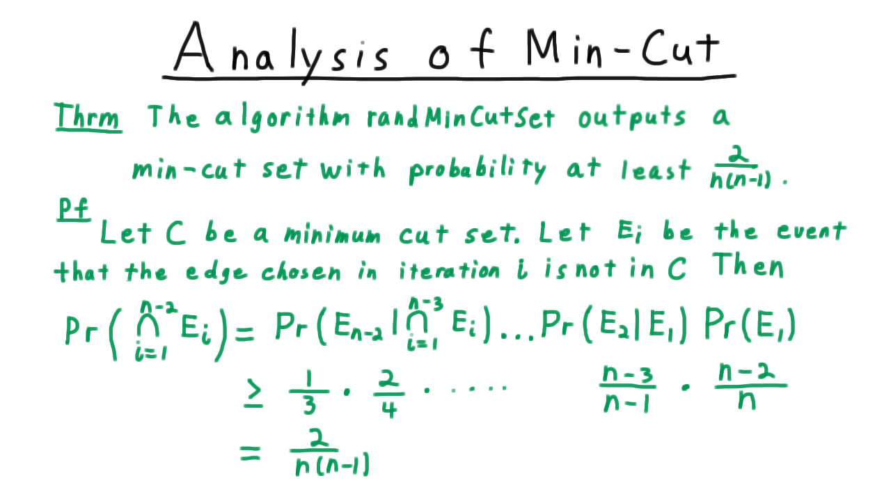
we see that we are down to a \(1/3\) probability in the last iteration, \(2/4\) in the iteration before than, etc. This product telescopes and leaves us with the bound of \(\frac{2}{n(n-1)}\) as claimed.

Altogether then, this extremely simple procedure has given us a fairly efficient algorithm for finding a minimum cut set.

Max 3 SAT - (Udacity, Youtube)

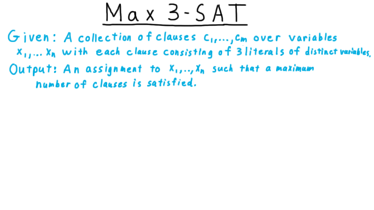
For our last algorithm we will consider maximum 3-SAT. This will tie together randomized algorithms, approximation algorithms, and complexity. We are given given a collection of clauses each with 3 literals, all coming from distinct variables. And we want to output an assignment to the variables such that a maximum number of clauses is satisfied.

First, we are going to show that

For any 3CNF formula there is an assignment that satisfies at least 7/8 of the literals.

Consider an assignment chosen uniformly at random. Define \(Y_j\) to be 1 if the clause \(c_j\) is satisfied and to be 0 otherwise. Since all the literals come from distict variables, then there are eight possible ways of assignment them true or false values, but only one of them will cause \(Y_j\) to be equal to 0. The rest satisfy the clause and cause \(Y_j\) to be 1. Thus, \(E[Y_j] = 7/8\) for every \(j.\)

Now we consider the formula as a whole and let \(Y = \sum_{j=1}^m Y_j\). Using the linearity of expectations, we have that
\[ \sum_{v \in Y(\Omega)} v \Pr(Y = v) = E[Y] = \sum_{j=1}^m E[Y_j] = m\frac{7}{8} \]

The key realization is that this value represents a kind of average. This mean that not all of the \(v\) in this sum on the left can be less than the average on the right. There has to be a \(v\) where the probability is positive and the value of \(v \geq 7m/8.\) Because this probability is positive, however, there must be some assignment to the variables that achieves it. Therefore, there is always a way to satisfy \(7/8\) of the clauses in any 3-SAT formula.

This technique of proof is called the “expectation argument” and it is part of a larger collection of very powerful tools called the probabilistic method, which were developed and popularized by the famous Paul Erdos.

Approx Max 3 SAT - (Udacity, Youtube)

So far, we’ve seen how there must be an assignment that satisfies at least 7/8 of the clauses in any 3-CNF formula, and in fact, the same argument gives us an algorithm that satisfies 7/8 on average: just pick a random assignment.

By itself, however, this does not provide any guarantee that we will actually find an assignment that satisfies 7/8 of the clauses. To obtain such a guarantee, we are going to use a technique called derandomization that will take randomness of the algorithm our and give us a deterministic algorithm with a guaranteed 7/8 factor approximation.

An important part of the algorithm will be a subroutine that assigns a value to a variable and simplifies the clauses. We will call this procedure instantiate.

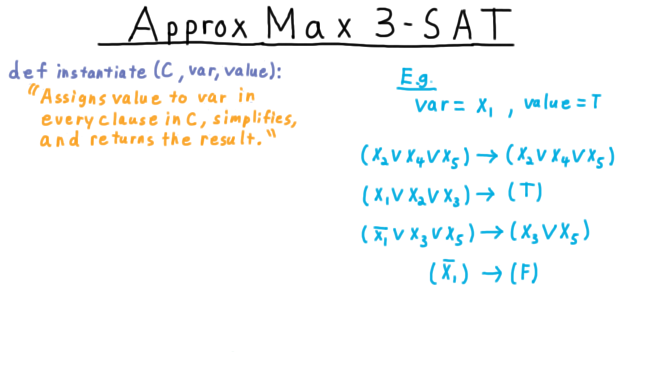
Let’s say that we set variable \(x_1\) to True. Then any clauses not using \(x_1\) are left alone. If a clause has \(x_1\) in it, then it gets set to True. If a clause has \(\overline{x_1}\) in it, then we just eliminate that literal from the clause. If the \(\overline{x_1}\) is the only literal in a clause, then we just set the clause to False.

Another important subroutine, will be one that calculates the expected number clauses that will be satisfied if the remaining variables are assigned True or False uniformly at random.

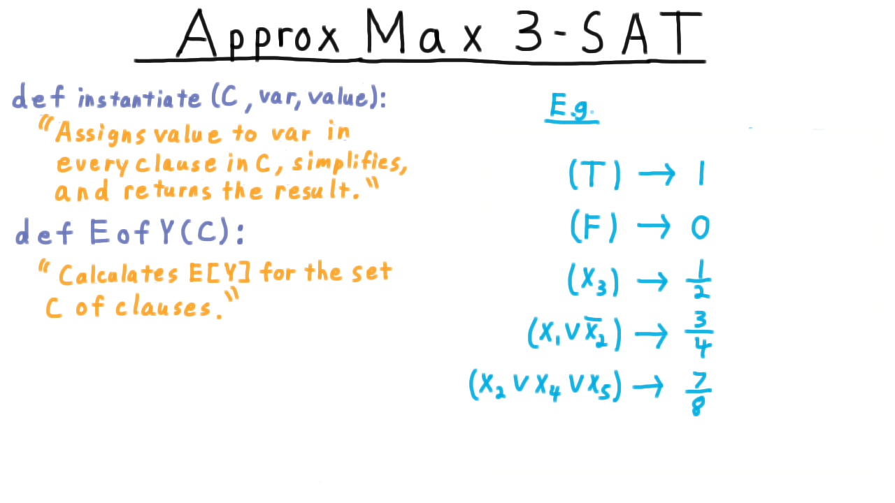
Of course, if a clause is just true, it gets assigned a value 1, false get assigned 0. A single literal gets assigned 1/2, two literals gets a value of 3/4 and three literals gets a value of 7/8. Remember that there is just one way to assign the relevant variables to that this clause is false. The EofY procedure simply calculates these values for every clause and sums them up.

With these subroutines defined, we can write down our derandomized algorithm as follows.

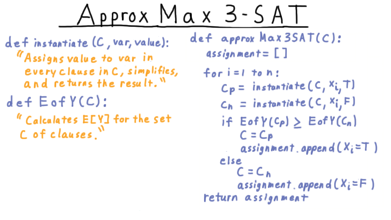
Start with an empty assignment to the variables. Then for each variable in turn, consider the formula resulting from its being set to True and its being set to False. Between these two, pick the one that gives a larger expected value for the number of satisfied clauses assuming that the remaining variables were set at random. Note that we are using our knowledge of how a random assignment would behave here, but we aren’t actually using any randomization. Having picked the better of the two ways of assigning the \(x_i\) variable, we update the set of clauses record our assignment to \(x_i.\)

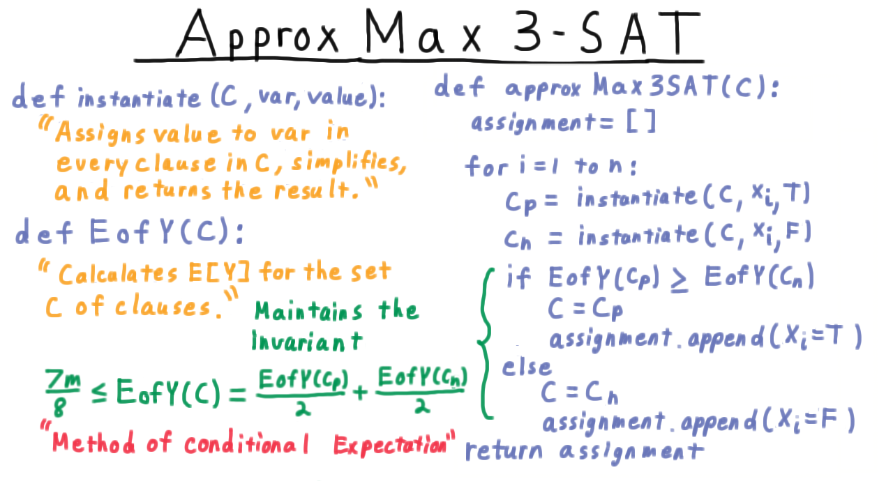
The reason this algorithm works is that it maintains the invariant that the expected number of clauses of \(C\) that would be satisfied if the remaining variable were assigned random is at least 7/8. This is true at the beginning, just by our previous theorem. But this expectation for \(C\) is always just the average of the expected number that would be satisfied in \(C_p\) and \(C_n.\) So by picking the new \(C\) to be the one for which this EofY quantity is larger, the invariant is maintained. Of course, at the end, all of the variables have been assigned, so this computing the expectation of \(C\) amounts to just counting up the number of True clauses. This technique is known as the method of conditional expectation and it has a number of clever applications.

Overall, then we have shown that there is a deterministic algorithm which give any 3-CNF formula finds an assignment that satisfies 7/8 of the clauses. Remarkably, it turns our that this is the best we can do assuming P is not equal to NP. For this argument, we turn to the celebrated and extremely popular PCP theorem.

PCP Theorem - (Udacity, Youtube)

PCP stands for probabilistically checkable proofs. It turns out that if you take the verifiers we talked about when we defined the class NP, and

1. you give them access to random bits, and

2. you give them random access into the certificate or proof

then they become extremely efficient. These types of verifiers are called probabilistically checkable proof systems, and the famous PCP theorem relates the set of languages they can verify under certain constraints back to the class NP.

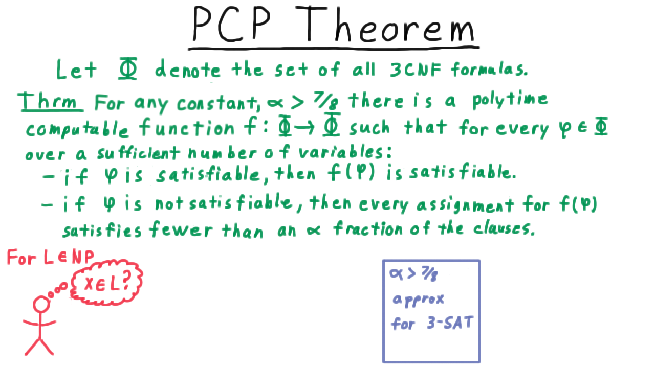
In a course on complexity, we would place these proof systems within the larger context of other complexity classes and interactive proof systems. For our purposes, however, the PCP theorem can be stated in this much more accessible way.We’ll let \(\Phi\) denote the set of all 3CNF formulas. Remember that we are assuming that all clauses have exactly 3 literals and that they come from 3 distinct variables. Then a version of the PCP theorem can be stated like this:

For any constant \(\alpha > 7/8\), there is a polytime computable function \(f \Phi \rightarrow \Phi\) such that for every 3CNF formula that has a sufficient number of variables, we have that

1. if \(\phi\) is satisfiable, then \(f(\phi)\) is satisfiable, and
2. if \(\phi\) is not satisfiable, then every assignment of the variables satisfies fewer than an \(\alpha\) fraction of the clauses.

So if \(\phi\) is satisfiable, there is a way to satisfy all the clauses of \(f(\phi)\). If \(\phi\) is unsatisfiable, then you can’t even get close to satisfying all the clauses of \(f(\phi).\) We’ve introduced a gap here, and this gap is extremely useful for proving the hardness of approximation.

Many, many hardness of approximation results follow from this theorem. The most straightforward of them, however, is that you can’t do better than the 7/8 algorithm for max-sat that we just went over–not unless P=NP. Why?

Well, suppose that I wanted to test whether strings were in some language in NP.
And at my disposal, I had a polytime alpha-approximation for 3-SAT, where alpha is strictly greater than 7/8.

Then, I could use the Cook-Levin reduction to transform my string into an instance of SAT that will be satisfiable if and only if x is in L.

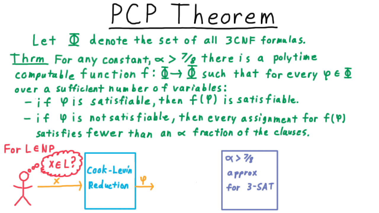
Then, I can use this f function from the PCP theorem to transform this into another 3SAT clauses where either all the clauses are satisfiable or fewer than an alpha fraction of them are.

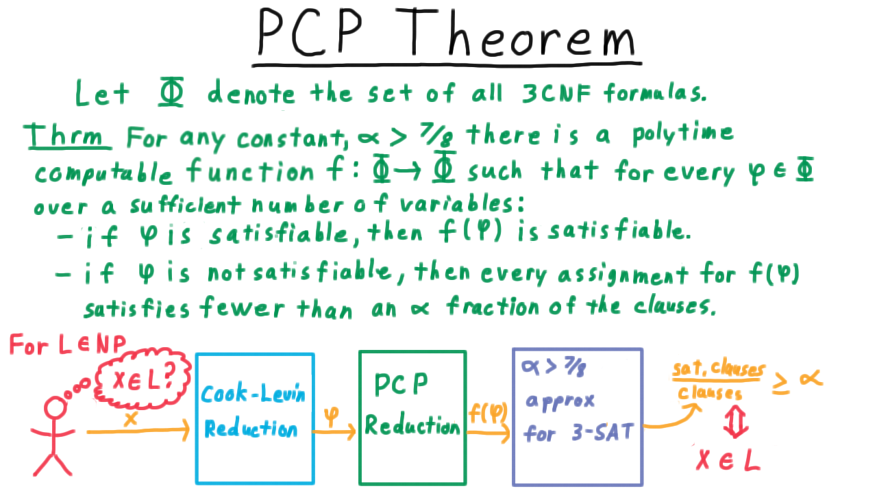
That way, I just run this \(\alpha\) approximation on \(f(\phi)\) and see if the fraction of clauses satisfied is at least than \(\alpha\) or not. If it is, then from the PCP theorem, I can reason that phi must have been satisfiable, and so from the Cook-Levin reduction \(x\) must have been in \(L.\)

On the other hand, if the fraction of satisfied clauses is less than \(\alpha,\) then \(f(\phi)\) cannot have been satisfiable, so \(\phi\) must not have been satisfiable, so from the Cook-Levin reduction \(x\) must not be in \(L.\)
Using this reasoning, we just found a way to decide an arbitrary language in NP in polynomial time. So if such an \(\alpha\) approximation exists, then P=NP. Or more likely, P is not equal to NP, so no such approximation algorithm can exist.

Many hardness of approximation proofs can be done in a similar way. All that’s necessary is to stick in another transformation here, transforming the 3SAT problem that has this gap into another problem, which might have a potentially different gap, to show that certain approximation factors would imply P=NP.

Conclusion - (Udacity, Youtube)

As we’ve seen, randomization can be a very useful tool in the design and analysis of algorithms, and it turns out that this is true in practical programming too, as many real-world computer programs rely on pseudorandomness to achieve their desired behavior. Nevertheless, it is an open question whether randomization actually helps in the sense of the complexity classes that we discussed earlier on in the course. It simply isn’t known whether there is a language that can be decided in polynomial time with a two-sided Monte-Carlo algorithm, that can’t be decided with a normal Turing machine in polynomial time. This is known as the P equals BPP question, and it’s one of the major open problems in Complexity.