Computability, Complexity, and Algorithms
Charles Brubaker and Lance Fortnow
Computability, Complexity, and Algorithms
Charles Brubaker and Lance Fortnow
P and NP - (Udacity)
Introduction - (Udacity, Youtube)
So far in the course, we have answered the question: what is computable? We modeled computability by Turing machines and showed that some problems, like the halting problem, cannot be computed at all.
In the next few lectures we ask, what can we compute quickly? Some problems, like adding a bunch of numbers or solving linear equations, we know how to solve quickly on computers. But how about playing the perfect game of chess? We can write a computer program that can search the whole game tree, but that computation won’t finish in our lifetime or even the lifetime of the universe. Unlike computability, we don’t have clean theorems about efficient computation. But we can explore what we probably can’t solve quickly through what known as the P versus NP problem.
P represents the problems we can solve quickly, like your GPS finding a short route to your destination. NP represents problems where we can check that a solution is correct, such as solving a Sudoku puzzle. In this lesson we will learn about P, NP, and their role in helping us understand what we may or may not be able to solve quickly.
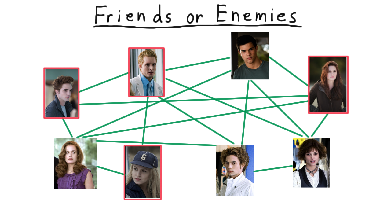
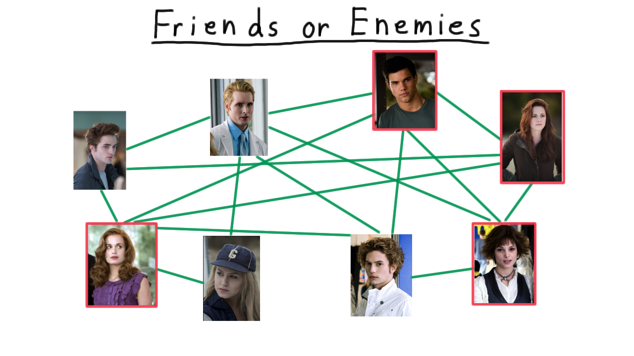
Friends or Enemies - (Udacity, Youtube)
We’ll illustrate the distinction between P and NP by trying analyze a world of friends and enemies. Everyone is this world is either a friend or an enemy, and we’ll represent this by drawing an edge between all of the friends like so.
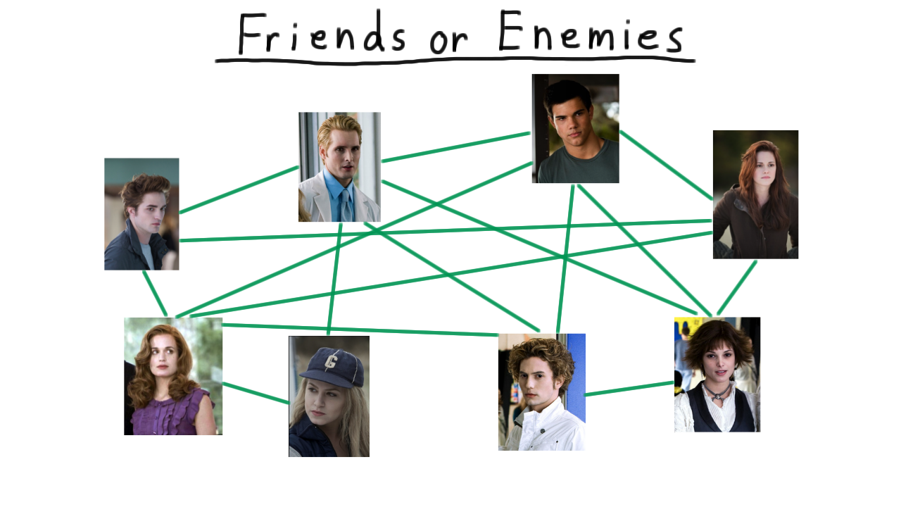
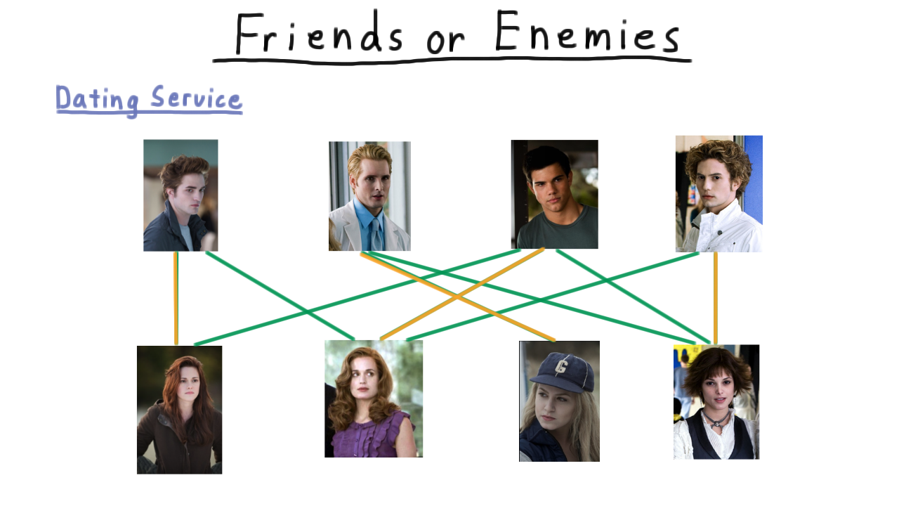
Given all this information, there are several types of analysis that you might want to do, some easier and some harder. For instance, if you wanted to run a dating service, you would be in pretty good shape. Say that you wanted to maximize the number of matches that you make and hence the number of happy customers. Or perhaps, you just want to know if it’s possible to give everyone a date. Well, we have efficient algorithms for finding matchings, and we’ll see some in a future lesson. Here, in this example, it’s possible to match everyone up, and such a matching is fairly easy to find.
Contrast this with problem of identifying cliques. By clique, I mean a set of people who are all friends with each other. For instance, here is a clique of size three: every pair of members has an edge between, and cliques of that size aren’t too hard to find.
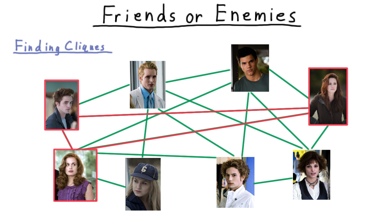
As we start to look for larger cliques, however, the problem becomes harder and harder to solve.
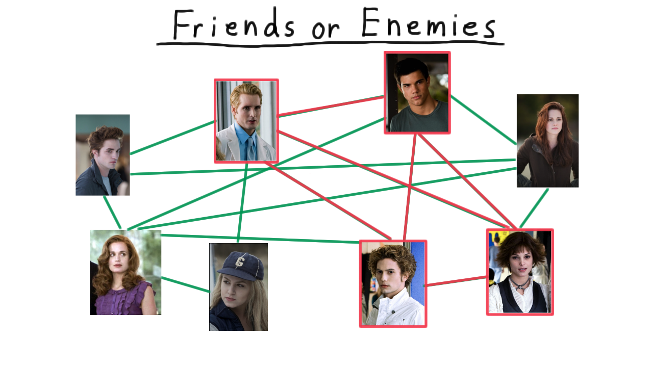
Find a Clique - (Udacity)
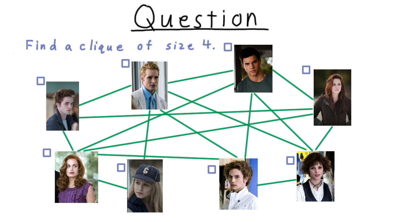
In fact, finding a clique of size four, even for a relatively small graph like this one isn’t necessarily easy. See if you can find one.
P and NP - (Udacity, Youtube)
Being a little more formal now, we define P to be the set of problems solvable in polynomial time. By polynomial time, we mean that the number of Turing machine steps is bounded a by a polynomial. We’ll formalize this more in a moment. Bipartite matching was one example of this class of problems.
NP we define as the class of problems verifiable in polynomial time. This includes everything in P, since if a problem can be solved in polynomial time, a potential solution can be verified in that time, too. Most computer scientists strongly believe that this containment is strict. That is to say, there are some problems that are efficiently verifiable but not efficiently solvable, but we don’t have a proof for this yet. The clique problem that we encountered is one of the problems that belongs in NP but we think does not belong in P.

There is one more class of problems that we’ll talk about in this section on complexity, and that is the set of NP-complete problems. These are the hardest problems in NP, and we call them the hardest, because any problem in NP can be efficiently transformed into an NP-complete problem. Therefore, if someone were to come up with a polynomial algorithm for even one NP-complete problem, then P would expand out in this diagram, making P and NP into the same class. Finding a polynomial solution for clique would do this, so we say that clique is NP-complete. Since solving problems doesn’t seem to be as easy as checking answers to problems, we are pretty sure that NP-complete problems can’t be solved in polynomial time, and therefore that P does not equal NP.
To computer science novices the difference between matching and clique might not seem to be a big deal and it is surprising that one is so much harder than the other. In fact, the difference between a polynomially solvable problem and a NP-complete one can be very subtle. Being able to tell the difference is an important skill for anyone who will be designing algorithms for the real world.
Delicacy of Tractability - (Udacity, Youtube)
As we discussed, one way to see the sublety of the difference between problems in P and those that are NP-complete is to compare what it takes to solve seemingly similar real-world problems.
Consider the shortest path problem. You are given two locations and you want to find the shortest valid route between them. You phone does this in a matter of milliseconds when you ask it for directions, and it gives you an exact answer according to whatever model for distance it is using. This is computationally tractable.
On the other hand, consider this warehouse scenario where a customer places an order for several different items and a person or a robot has to go around and collect them before going to the shipping area for them to be packed. This is called the traveling salesman problem and it is NP-complete. This problem also comes up in the unofficial guide to Disney World, which tries to tell you how to get to all the rides as quickly as possible.
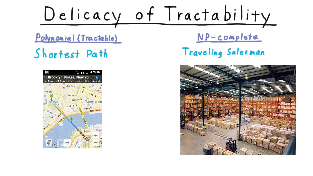
This explains why your phone can give you directions but supply chain logistics–just figuring out how things should be routed– is a billion dollar industry.
Actually, however, we don’t even need to change the shortest path so much to get an NP-complete problem. Instead of asking for the shortest path, we could ask for the longest, simple path. We have to say simple so that we don’t just go around in cycles forever.
This isn’t the only possible pairing of similar P and NP-complete problems either. I’m going to list some more. If you aren’t familiar with these problems yet, don’t worry. You will learn about them by the end of the course. Vertex cover in bipartite graphs in polynomial, but vertex cover in general graphs is NP complete.
An class of optimization problems called Linear Programming is in P, but if we restrict the solutions to integers, then we get an NP-complete problem Finding an Eulerian cycle in a graph where you touch each edge once is polynomial. On the other hand, finding a Hamiltonian cycle that touches each vertex once is NP-complete
And lastly, figuring out whether a boolean formula with two literals per clause is polynomial, but if there are three literals per clause, then the problem is NP-complete.

Unless you are familiar with some complexity theory, problems in P aren’t always easy to tell from those that are NP-complete. Yet, in the real world when you encounter a problem it is very important to know which sort of problem you are dealing with. If your problem is like one of the problems in P, then you know that there should be an efficient solution and you can avail yourself of the wisdom of many other scientists who have thought hard about how to efficiently solve these problems. On the other hand, if your problem is like one the NP-complete problems, then some caution is in order. You can expect to be able to find exact solutions for small enough instances, and you may be able to find a polynomial algorithm that will give an approximate solution that is good enough, but you should not expect to find an exact solution that will scale well for all cases.
Being able to know which situation you are in is one of the main practical benefits of studying complexity.
Running Time Analysis - (Udacity, Youtube)
Now, we are going to drill down into the details and make many of the notions we’ve been talking about more precise. First we need to define running time.
We’ll let M be a Turing machine– single-tape, multi-tape, random access, the definition works for all of them. The running time of the machine then is a function over the natural numbers where f(n) is the largest number of steps taken by the machine for an input string of length n. We can extend this definition to machines that don’t halt as well by making their running time infinite. We always consider the worst case.
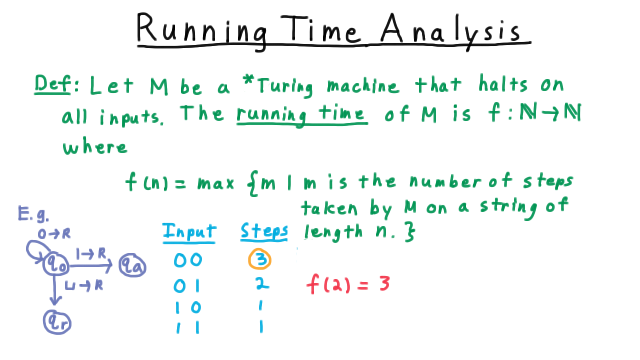
Let’s illustrate this idea with an example. Consider the single-tape machine in the figure above that takes binary input and tests whether the input contains a 1. Let’s figure out the running time for string of length 2. We need to consider all the possible strings of length 2, so we make a table and count the number of steps. The largest number of steps in 3, where we read both zeros and then the blank symbol. Therefore, f(2) = 3.
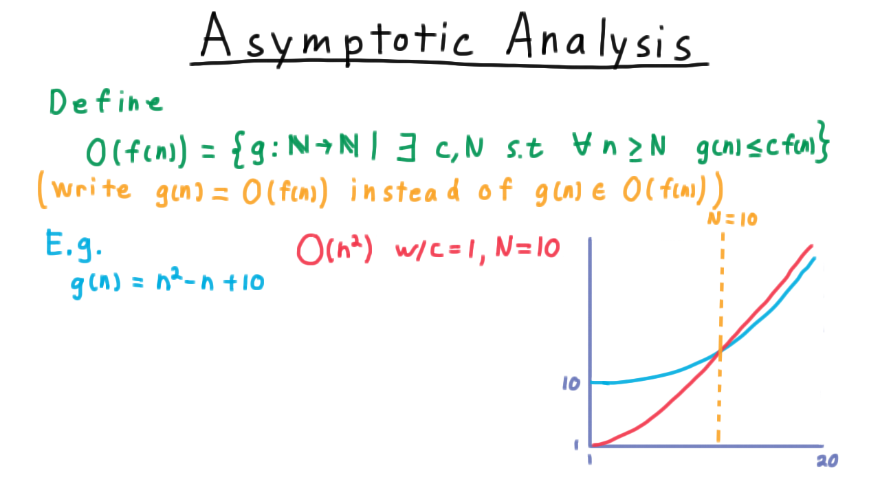
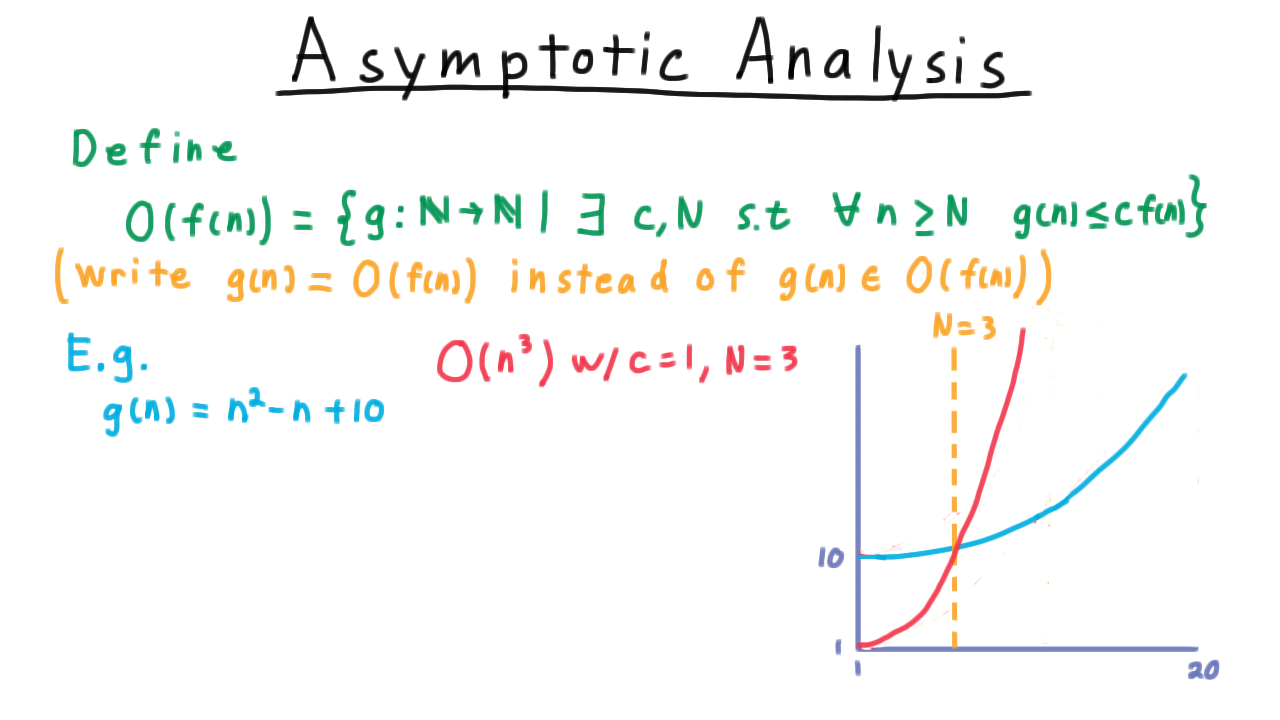
Asymptotic Analysis - (Udacity, Youtube)
Now, it’s not very practical to write down every running time function exactly, so computer scientists use various levels of approximation. For complexity, we use asymptotic analysis. We’ll do a very brief review here, but if you haven’t seen this idea before you should take a few minutes to study it on your own before proceeding with the lesson.
In words, the set \(O(f(n))\) is the set of functions \(g\) such that \(g \leq cf(n)\) for sufficiently large \(n\). Making this notion of “sufficiently large \(n\)” precise, we end up with
Even though we’ve defined \(O(f(n))\) as a set, we write \(g(n) = O(f(n))\) instead of using the inclusion sign. We also say that \(g\) is order \(f\).
This definition can be a little confusing, but it should feel like the definition of a limit from your calculus class. In fact, we can restate this condition to say that the ratio of \(g\) over \(f\) converges to a constant under the limsup.
An example also helps. Take the function \(g(n) = n^2 - n + 10.\)
We can argue that this is order \(n^2\) by choosing \(c = 1\) and \(N = 10\). For every \(n \geq 10\) , \(n^2\) is greater than the function \(g\).
We also could have chosen \(c = 10\) and \(N = 1.\)
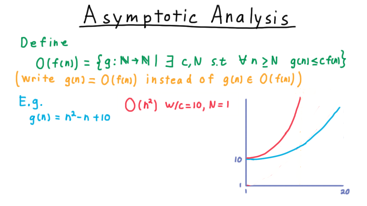
Note that the big-O notation does not have to create a tight bound. Thus, \(g = O(n^3)\) too. Setting \(c= 1\) and \(N= 3\) works for this.
Big O Question - (Udacity)
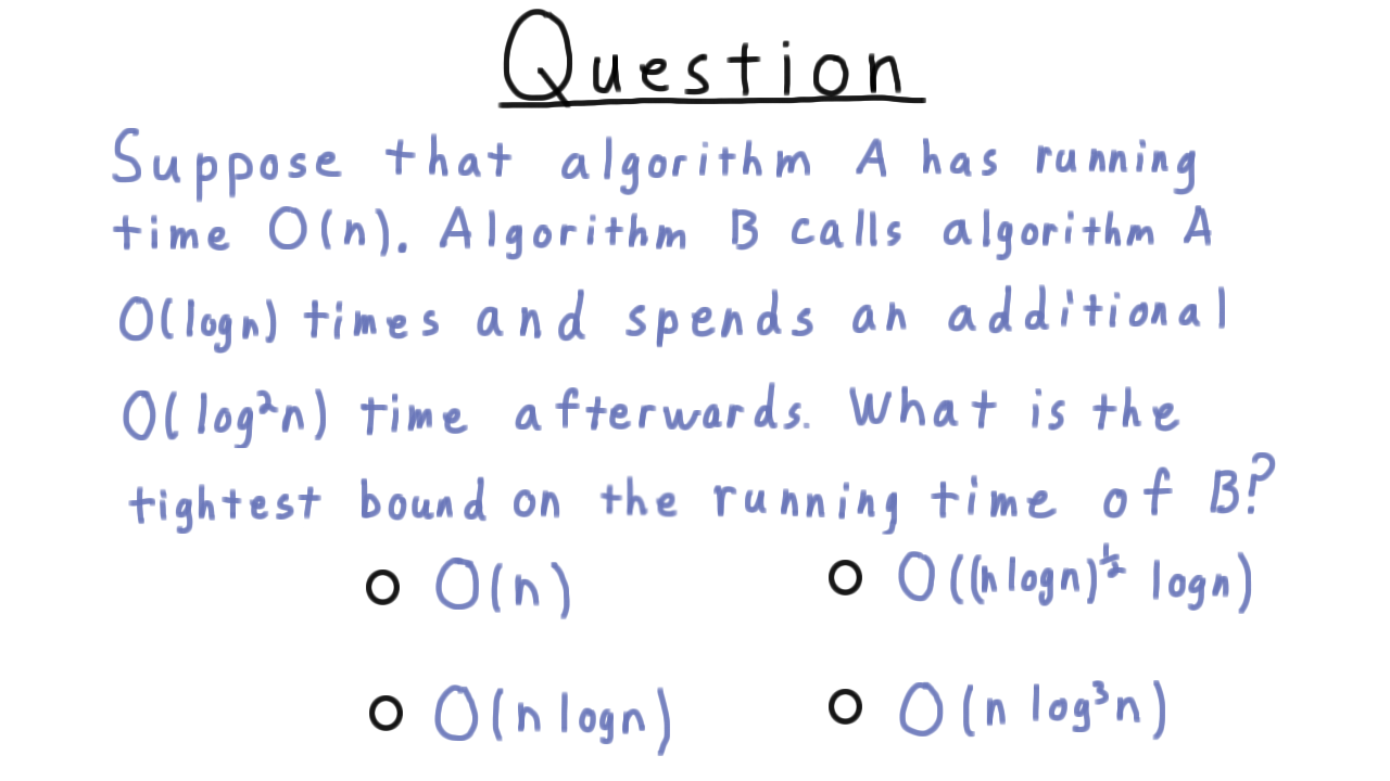
Once we’ve established the running time for an algorithm, we can analyze other algorithms that use it as a subroutine much more easily. Consider this question. Suppose that algorithm A has running time O(n), and A is called by algorithm B O(log n) times, and algorithm B runs for an additional log-squared n time afterwards. What is the tightest bound on the running time of B?
The Class P - (Udacity, Youtube)
We are now ready to formally define the class P. Most precisely,
P is the set of languages recognized by an order \(n^k\) deterministic Turing machine for some natural number \(k\).
There are several important things to note about this definition.
- First is that P is a set of languages. Intuitively, we talk about it as a set of problems, but to be rigorous we have to ultimately define it in terms of languages.
- Second is the word deterministic. We haven’t seen a non-deterministic Turing machine yet, but one is coming. Deterministic just means that given a current state and tape symbol being read, there is only one transition for the machine to follow.
- An \(n^k\) time machine here is one with running time order \(n^k\) as we defined these terms a few minutes ago.

Perhaps the most interesting thing about this definition is the choice for any \(k\) in the natural numbers. Why is this the right definition? After all, if \(k\) is 100 then deciding the language isn’t tractable in practice.
The answer is that P doesn’t exactly capture what is tractable in practice. It’s not clear that any mathematical definition would stand the test of time in this regard, given how often computers change, or be relevant in so many contexts. This choice does have some very nice properties however.
- It matches tractability better than one might think. In practice, k is usually low for polynomial algorithms, and there are plenty of interesting problems not known to be in P.
- The definition is robust to changes to the model. That is to say, P is the same for single-tape, multi-tape machines, Random Access machines and so forth. In fact, we pointed out that the running times for each of those models are polynomially related when we introduced them.
- P has the nice property of closure under the composition of algorithms. If one algorithm calls another algorithm as a subroutine a polynomial number of times, then that algorithm is still polynomial, and the problem it solves is in P. In other words, if we do something efficient a reasonably small number of times, then the overall solution will be efficient. P is exactly the smallest class of problems containing linear time algorithms and which is closed under composition.
Problems and Encodings - (Udacity, Youtube)
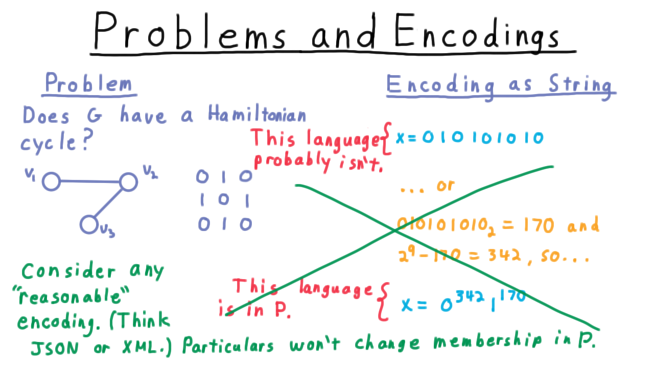
We’ve defined P as a set languages, but ultimately, we want to talk about it as a set of problems. Unfortunately, this isn’t as easy as it might seem. The encoding rules we use for turning abstract problems into strings can affect whether the language is in P or not. Let’s see how this might happen.
Consider the question: Does G have a Hamiltonian cycle–a cycle that visits all of the vertices? Here is a graph and here is its adjacency matrix.

A natural way to represent the graph as a string is to write out its adjacency matrix in scanline order as done in the figure above. But this isn’t the only way to encode the graph. We might do something rather inefficient.
The scanline encoding for this graph represents the number 170 in binary. We could choose to represent the graph in essentially unary.
We might represent the graph as 342 zeros followed by 170 ones. The fact that there are 29=512 symbols total indicates that it’s a 3x3 matrix, and converting 170 back into binary gives us the entries of the adjacency matrix.

This is a very silly encoding, but there is nothing invalid about it.
This language, it turns out, is in P, not because it allows the algorithm to exploit any extra information or anything like that, but just because the input is so long. The more sensible, concise encoding isn’t known to be in P (and probably isn’t, by an overwhelming consensus of complexity theorists). Thus, a change in encoding can affect whether a problem is in P, yet it’s ultimately problems that we are interested in, independent of the particulars of the encoding.
We deal with this problem, essentially by ignoring unreasonable representations like this one. As long as we consider any reasonable encoding (think about what xml or json would produce from how you would store it in computer memory) then the particulars won’t change the membership of the language in P, and hence we can talk at least informally about problems being in P or not.
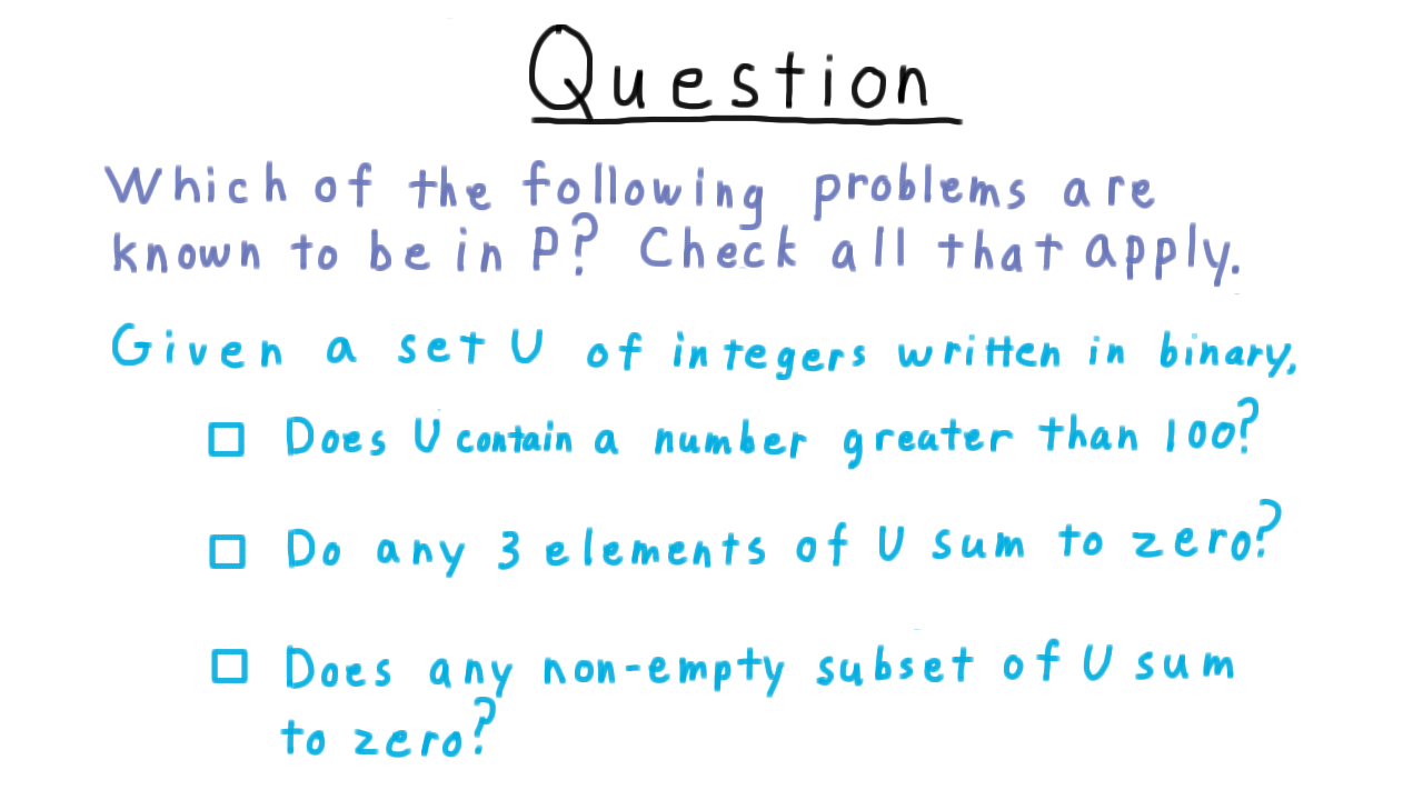
Which are in P - (Udacity)
Now that we have defined P, I want to illustrate how easy it can be to recognize that a problem is in P. Recognizing that a problem is NOT in P is a little harder, so for this exercise assume that if the brute-force algorithm is exponential, so is the best algorithm. Consider a finite set U of the integers and the following three problems. Check the ones that you think are in P. (Again, if there isn’t an obvious polynomial-time algorithm, assume that there isn’t one.)
Nondeterministic TMs - (Udacity, Youtube)
From the class P, we now turn to the class NP. At the beginning of the lesson, I said that NP is the class of problems verifiable in polynomial time. This is true, but it’s not how we typically define it. Instead, we define NP as the class of problems solvable in polynomial time on a nondeterministic Turing machine, a variant that we haven’t encountered before.
Nondeterminism in computer science is often misunderstood, so put aside whatever associations you might have had with the word. Perhaps the best way to understand nondeterministic Turing machines is by contrasting a nondeterministic computation with a deterministic one. A deterministic computation starts in some initial state and then the next state is exactly uniquely determined by the transition function. There is only one possible successor configuration.
And to that configuration there is only one possible successor.
And so on and so forth. Until an accepting or rejecting configuration is reached, if one is reached at all.

On the other hand, in a nondeterministic computation, we start in a single initial configuration, but it’s possible for there to be multiple successor configurations. In effect, the machine is able to explore multiple possibilities at once. This potential splitting continues at every step. Sometimes there might just be one possible successor state, sometimes there might be three or more. For each branch, we have all the same possibilities as for a deterministic machine.
- It can reject.
- It can loop forever.
- It can accept.
If the machine ever accepts in any of the these branches, then the whole machine accepts.
The only change we need to make to the 7-tuple of the deterministic Turing machine needed to make it nondeterministic is to modify the transition function. An element of the range is no longer the set of single (state, tape-symbol to write, direction to move) tuple, but a collection of all such possibilities.
\[ \delta: Q \times \Gamma \rightarrow \{S \; | \; S \subseteq Q \times \Gamma \times \{L,R\} \} \]
This set of all subsets used in the range here is often called a power set.
The only other change that needs to be made is when the machine accepts. It accepts if there is any valid sequence of configurations that results in an accepting state. Naturally, then it also rejects only when every branch reaches a reject state. If there is a branch that hasn’t rejected yet, then we need to keep computing in case it accepts.
Therefore, a nondeterministic machine that never accepts and that loops on at least one branch will loop.
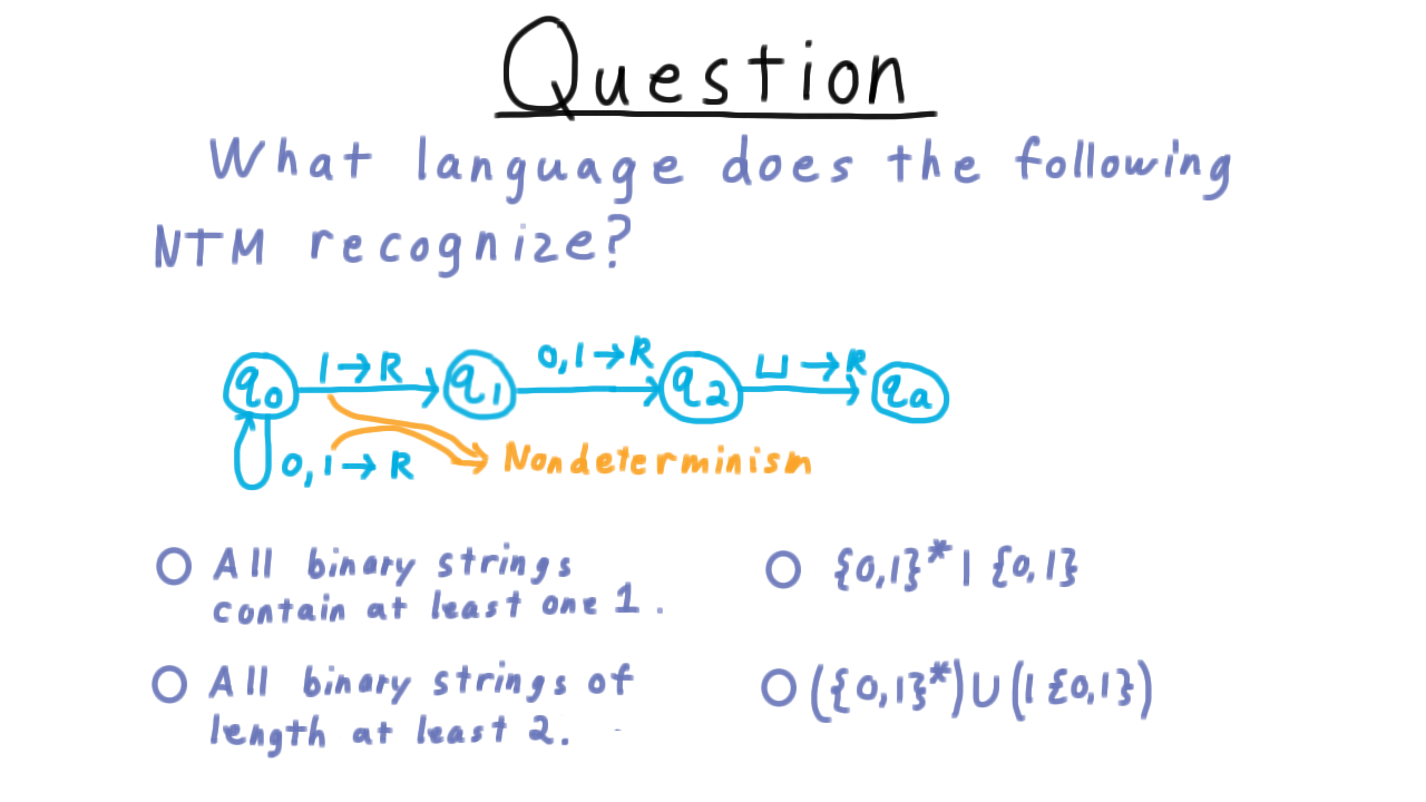
Which Language - (Udacity)
Here is the state transition diagram for a simple nondeterministic Turing machine. The machine starts out in \(q_0\) and then it can move the head to right on 0s and 1s, OR on a 1, it can transition to state \(q_1.\)
The fact that there are two transitions out of state \(q_0\) when reading a 1 is the nondeterministic part of the machine. In branches where the transition to state \(q_1\) is followed, the Turing machine reads one more 0 or 1 and then expects to hit the end of the input. Remember that by convention, if there is no transition specified in one of these state diagrams, then the machine simply moves to the reject state and halts. That keeps the diagrams from getting cluttered.
My question to you then is what language does this machine recognize? Check the appropriate answer.
Composite Numbers - (Udacity, Youtube)
To get more intuition for the power of nondeterminism, let’s see how much more efficient it makes deciding the language of composite numbers–that is, numbers that are not prime. The task is to decide the string representations of numbers that are the product of two positive integers, greater than 1.
One deterministic solution looks like this.

Think of the flow diagram as capturing various modules within the deterministic Turing machine. We start by initializing some number \(p\) to 1. Then we increment it, and test whether p-squared is greater than \(x\). If it is, then trying larger values of p won’t help us, and we can reject. If p-squared is no larger than \(x\), however, then we test to see if p divides x. If it does, we accept. If not, the we go try the next value for \(p.\)
Each iteration of this loop require a number of steps that is polynomial in the number of bits used to represent x. The trouble is that we might end up needing \(\sqrt{x}\) iterations of this outer loop here in order to find the right p or confirm that one doesn’t exist. This what makes the deterministic algorithm slow. Since the value of x is exponential in its input size–remember that it is represented in binary–this deterministic algorithm is exponential.
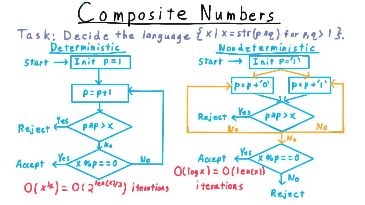
On the other hand, with nondeterminism we can do much better. We initialize p so that it is represented on it’s own tape as the number 1 written in binary. Then we nondeterministically modify \(p.\) By having two possible transitions for the same state and symbol pair, we can non-deterministically append a bit to p. (The non-deterministic transitions are in orange.)
Next, we check to see if we have made \(p\) too large. If we did, then there is no point in continuing, so we reject.
On the other hand, if \(p\) is not too big, then we nondeterministically decide either to
- append a zero to \(p\),
- append a 1 to \(p\), or
- leave \(p\) as it is and go see if it divides \(x.\)
If there is some p that divides \(x\), then some branch of the computation will set \(p\) accordingly. That branch will accept and so the whole machine will. On the other hand, if no such \(p\) exists, then no branch will accept and the machine won’t either. In fact, the machine will always reject because every branch of computation will be rejected in one of the two possible places.
This non-deterministic strategy is faster because it only requires \(\log x\) iterations of this outer loop. The divisor \(p\) is set one bit at a time and can’t use more bits than \(x,\) the number it’s supposed to divide.
Thus, while the deterministic algorithm we came up with was exponential in the input length, it was fairly easy to come up with a nondeterministic one that was polynomial.
The Class NP - (Udacity, Youtube)
We are almost ready to define the class NP. First, however, we need to define running time for a nondeterministic machine, because it operates differently from a deterministic one.
Since we think about all of these possible computations running in parallel, the running time for each computational path is the path length from the initial configuration.
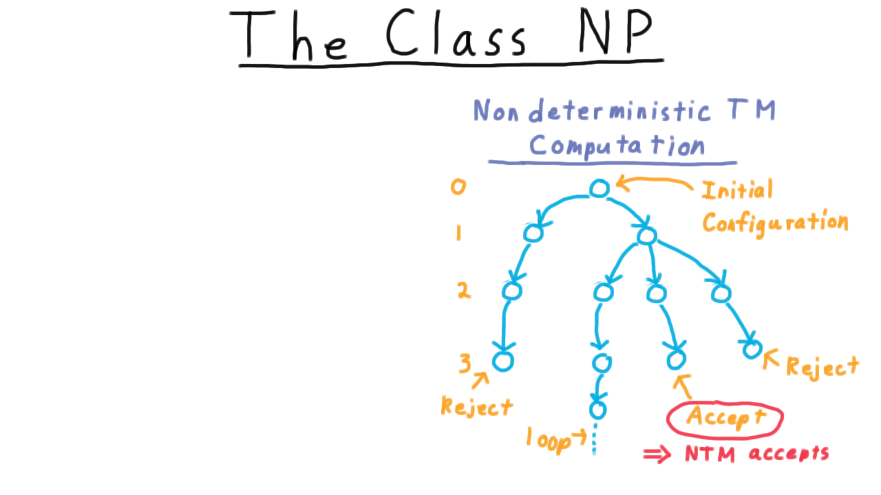
And the running time of the machine as a whole is the maximum number of steps used on any branch of the computation. Note that once we have a bound the length of any accepting configuration sequence, we can avoid looping by just creating a timeout.
NP is the set of languages recognized by an \(O(n^k)\) time nondeterministic Turing machine for some number \(k.\)
In other words, it’s the set of languages recognized in polynomial time by a nondeterministic machine. NP stands for nondeterministic polynomial time.
Nondeterminism can be a little confusing, but it helps to remember that a string is recognized if it leads to any accepting computation–i.e. any accepting path in this tree. Note that any Turing machine that is a polynomial recognizer for a language can easily be turned into a polynomial decider by adding a timeout since all accepting computations are bounded in length by a polynomial.
NP Equals Verifiability Intuition - (Udacity, Youtube)
At the beginning of the lesson, we identified NP as those problems for which answer can be verified in polynomial time. Remember how easy it was to check that a clique was a clique? In the more formal treatment, however, we defined NP as those languages recognized by nondeterministic machines in polynomial time. Now we get to see why these mean the same thing.
To get some intuition, we’ll revisit the example of finding a clique of size 4. We already discussed how a clique of size 4 is easy to verify, but how is it easy to find it with a non-deterministic machine? The key is to use the non-determinism to create a branch of computation for each subset of size 4, and then use our verification strategy to decide whether any of those subsets corresponds to a clique.
Remember that if any sequence of configurations accepts, then the non-deterministic machine accepts.
One branch of computation might choose these 4 and then reject because it’s not a clique.
Another branch might choose these 4 and also reject.
But one branch will choose the correct subset and this will accept.
And, that’s all we need. If one branch accepts then the whole non-deterministic machines does, as it should. There is a clique of size 4 here.
NP Equals Verifiability - (Udacity, Youtube)
Now for the more formal argument.
A verifier for a language \(L\) is a deterministic Turing machine \(V\) such that \(L\) is equal to the set of strings \(w\) for which there is another string \(c\) such that \(V\) accepts the pair \((w,c).\)
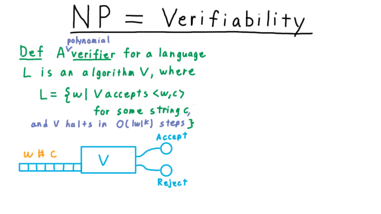
In other words, for every string \(w \in L\), there is a “certificate” c that can be paired with it so that V will accept, and for every string not in \(L\), there is no such string \(c\). It’s intuitive to think of \(w\) as a statement and of \(c\) as the proof. If the statement is true, then there should be a proof for it that \(V\) can check. On the other hand, if \(w\) is false, then no proof should be able to convince the verifier that it is true.
A verifier is polynomial if it’s running time is bounded by a polynomial in \(w.\)
Note that this \(w\) is the same one as in the definition. It is the string that is a candidate for the language. If we included the certificate \(c\) in the bound, then it becomes meaningless since we could make \(c\) be as long as necessary. That’s a polynomial verifier.
We claim
The set of Languages that have polynomial time verifiers is the same as NP.
The key to understanding this connection is once again this picture of the tree of computation performed by the nondeterministic machine.
If a language is in NP, then there is some nondeterministic machine that recognizes it, meaning that for every string in the language there is an accepting computation path. The verifier can’t simulate the whole tree of the nondeterministic machine in polynomial time, but it can simulate a single path. It just needs to know which path to simulate.
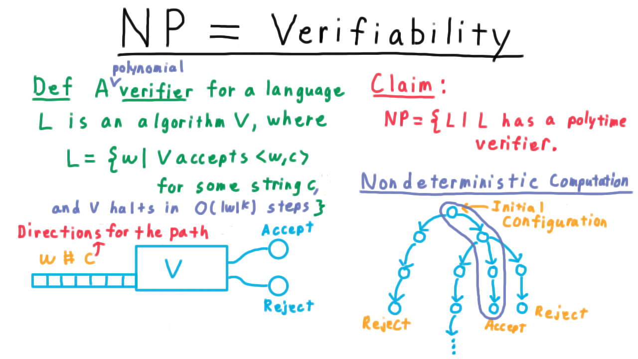
But this is what the certificate can tell it. The certificate can act as directions for which turns to make in order to find the accepting computation of the nondeterministic machine. Hence, if there is nondeterministic machine that can recognize a language, then there is a verifier that can verify it.
Now, we’ll argue the other direction. Suppose that V verifies a language. Then, we can build a nondeterministic machine whose computation tree will look a bit like a jellyfish. It the very top, we have a high degree of branching as the machine nondeterministically appends a certificate c to its input.
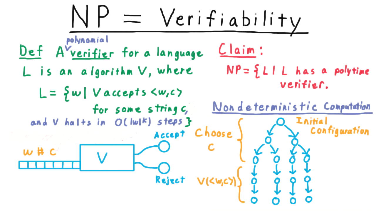
Then it just deterministically simulates the verifier. If there is any certificate that causes V to accept, the nondeterministic machine will find it. If there isn’t one, then the nondeterministic machine won’t.
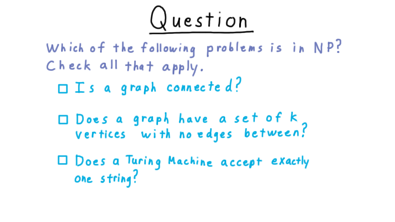
Which is in NP - (Udacity)
Now that we’ve defined NP and defined what it means to be verifiable in polynomial time, I want you to apply this knowledge to decide if several problems are in NP. First, is a graph connected? Second, does a graph have a set of k vertices with no edges between? This is called the independent set problem. And lastly, will a given Turing machine M accept exactly one string?
Conclusion - (Udacity, Youtube)
In this lesson, we have introduced the P and NP classes of problems. As we said in the beginning, the class P informally captures the problems we can solve efficiently on a computer, and the class NP captures those problems whose answer we can verify efficiently on a computer. Our experience with finding a clique in a graph suggests that these two classes are not the same. Cliques are hard to find but they are easy to check. And it is simply intuitive that solving a difficult problem should be harder than just checking a solution.
Nevertheless, no one has been able to prove that P is not equal to NP. Whether these two classes are equivalent is the known as the P versus NP question, and it is the most important open problem in theoretical computer science today if not in all of mathematics. We’ll discuss the full implications of the question in a later lecture, but for now, I’ll just mention that in the year 2000, the Clay Math Institute named the P versus NP problem as one of the seven most important open questions in mathematics and has offered a million-dollar bounty for a proof that determines whether or not P = NP. Fame and fortune await the person who settles the P v NP problem, but many have tried and failed.
Next class we look at the NP-complete problems, the hardest problems in NP.