Computability, Complexity, and Algorithms

Charles Brubaker and Lance Fortnow

NPC Problems - (Udacity)

Introduction - (Udacity, Youtube)

In the last lecture, we proved the Cook-Levin theorem which shows that CNF Satisfiability is NP-complete. We argued directly that an arbitrary problem in NP can be turned into the satisfiability problem with a polynomial reduction. Of course, it is possible to make such a direct argument for every NP-complete problem, but usually this isn’t necessary. Once we have one NP-complete problem, we can simply reduce it to other problems to show that they too are NP-complete.

In this lesson, we’ll use this strategy to prove that a few more problems are NP-complete. The goal is to give you a sense of the breadth of the class of NP-complete problems and to introduce you to some of the types are arguments used in these reductions.

Basic Problems - (Udacity, Youtube)

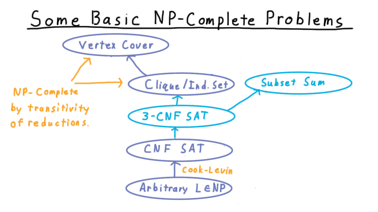
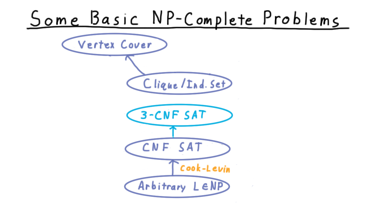
Here is the state of our knowledge about NP-complete problems given just what we proved in the last lesson.

We’ve shown that we can take an arbitrary problem in NP and reduce it to CNF satisfiability–that is what the Cook-Levin theorem showed.
We also did another polynomial reduction, one of the Independent Set/Clique problem to the Vertex Cover problem. Again, I’m treating Independent Set and Clique here as one, because the problems are so similar. Much of this lesson will be concerned with connecting up these two links into a chain.

First we are going to reduce general CNF-SAT to 3-SAT where each clause has exactly three literals. This is a critical reduction because 3-SAT is much easier to reduce to other problems than general CNF. Then we are going to reduce 3-CNF to Independent Set, and by transitivity this will show that vertex cover is NP-complete. Note that this is very convenient because it would have been messy to try to reduce every problem in NP to these problems directly. Finally, we will reduce 3-CNF to the Subset Sum problem, to give you a fuller sense of the types of arguments that go into reductions.

CNF 3CNF - (Udacity)

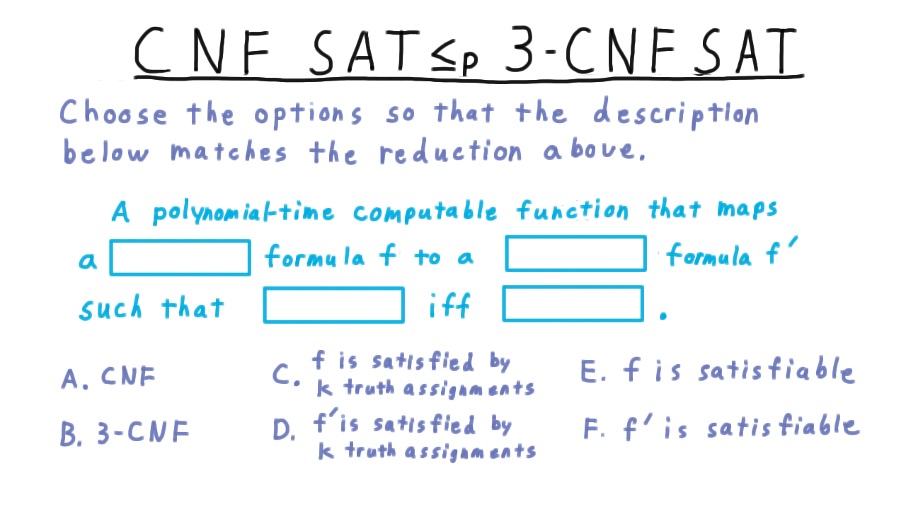
First we are going to reduce general CNF-SAT to 3-CNF-SAT. Before we begin however, I want you to help me articulate what we are trying to do. Here is a question. Choose from the options at the bottom and enter the corresponding letter in here so that this description matches the reduction we are trying to achieve.

Strategy and Warm up - (Udacity, Youtube)

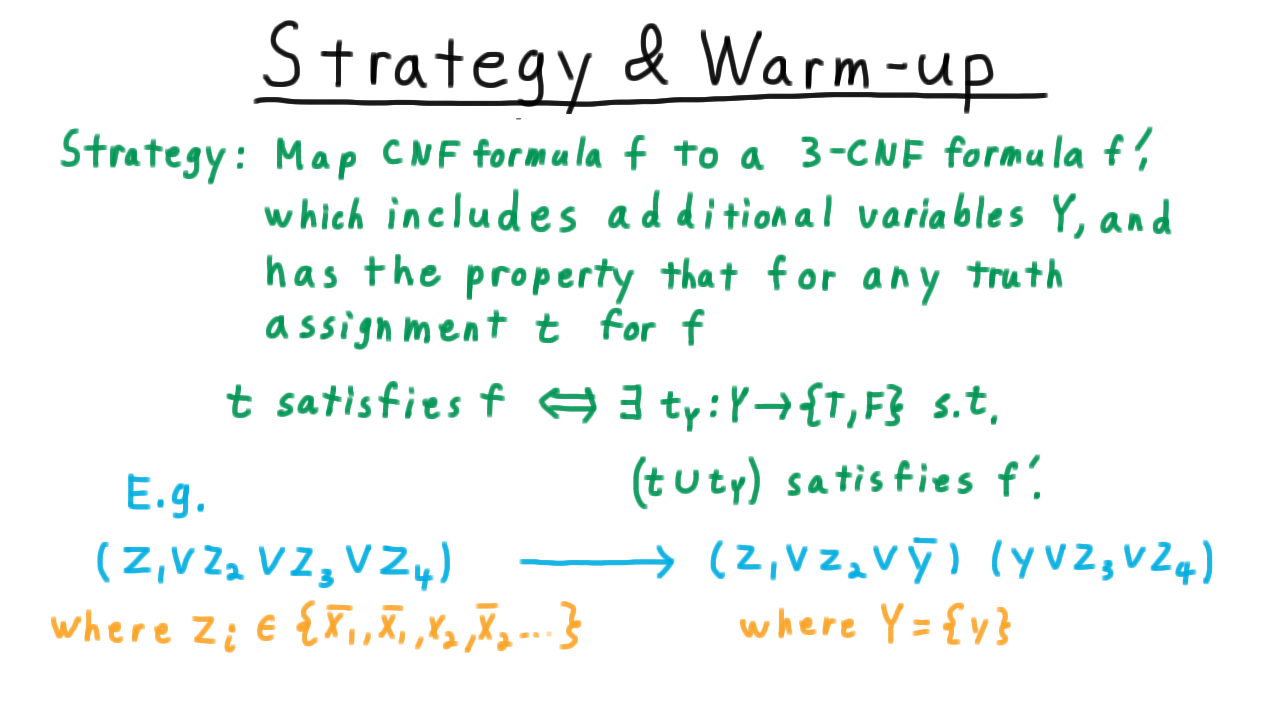
Here is our overall strategy. We’re going to take a CNF formula \(f\) and turn it into a 3CNF formula \(f',\) which will includes some additional variables, which we’ll label \(Y.\) This formula \(f'\) will have the property that for any truth assignment \(t\) for the original formula \(f,\) \(t\) will satisfy \(f\) if and only if there is a way \(t_Y\) of assigning values to \(Y\) so that \(t\) extended by \(t_Y\) satisfies \(f'.\)

Let’s illustrate such a mapping for a simple example. Take this disjunction of 4 literals.

\[(z_1 \vee z_2 \vee z_3 \vee z_4) \]

Note that the \(z_i\) are literals here, so they could be \(x_1\) or \(\overline{x_1}\), etc. Remember too that disjunction means logical OR; the whole clause is true if any one of the literals is.

We will map this clause of 4 into two clauses of 3 by introducing a new variable \(y\) and forming the two clauses

\[(z_1 \vee z_2 \vee \overline{y}) \wedge (y \vee z_3 \vee z_4).\]

Let’s confirm that the desired property holds. If the original clause is true, then we can set \(y\) to be \(z_1 \vee z_2\). If \(z_1 \vee z_2\) is true, then this first clause will be true by itself, and \(y\) can satisfy the other clause. Going the other direction, suppose that we have a truth assignment that satisfies both of these clauses. Suppose first that \(y\) is true. That implies that \(z_1 \vee z_2\) is true and therefore, the clause of four literals is. Next, suppose that \(y\) is false. Then \(z_3\) or \(z_4\) must true, and again so must the clause of four. If you have understood this, then you have understood the crux of why this reduction works. More details to come.

Transforming One Clause - (Udacity, Youtube)

We are going to start by looking at how to convert just one clause from CNF to 3-CNF. This is going to be the heart of the argument, because we will be able to apply this procedure to each clause of the formula independently. Therefore, consider one clause consisting of literals \(z_1\) through \(z_k.\) We are going to have four cases depending on the number of literals in the clause.

The case where \(k=3\) is trivial since nothing needs to be done.

When there are two literals in a clause, the situation is as simple trick suffices. We just need to boost up the number of literals to three. To do this, we include a single extra variable and trade in the clause

\[ (z_1 \vee z_2)\]

for these two clauses,

\[ (z_1 \vee z_2 \vee y_1) \wedge (z_1 \vee z_2 \vee \overline{y_1})\]

one with the literal \(y_1\) and one with the literal \(\overline{y_1}.\) If in a truth assignment \(z_1 \vee z_2\) is satisfied, then clearly both of these clauses have to be true. On the other hand, taking a satisfying assignment for the pair of clauses, the y-literal has to be false in one of them, so \(z_1 \vee z_2\) must be true.

We can play the same trick when there is just one literal \(z_1\) in the original clause. This time we need to introduce two new variables, which we’ll call \(y_1\) and \(y_2.\) Then we replace the original clause with four. See the chart below.

Note that if \(z_1\) is true, then all of collection of four clauses are true too. On the other hand, for any given truth assignment for \(z_1, y_1,\) and \(y_2\) that satisfies these clauses, the y-literals will have both be false in one of the four clauses. Therefore, \(z_1\) must be true.

Lastly, we have the case where \(k > 3\). Here we introduce \(k-3\) variables and use them to break up the clauses according to the pattern shown above.

Let’s illustrate the idea with this example

\[(z_1 \vee z_2 \vee z_3 \vee z_4 \vee z_5 \vee z_6).\]

Looking at this we might wish that we could have a single variable that captured whether any one of these first 4 variables were true. Let’s call this variable \(y_3.\) Then we could express this clause in as the 3 literal clause

\[(y \vee z_5 \vee z_6).\]

At first, I said we wanted \(y_3\) would to be equal to \(z_1 \vee z_2 \vee z_3 \vee z_4,\) but it’s actually sufficient, and considerably less trouble, for \(y_3\) to just imply it. This idea is easy to express as a clause.

\[(z_1 \vee z_2 \vee z_3 \vee z_4 \vee \overline{y})\]

Either y is false, in which case this implication doesn’t apply, or one of \(z_1\) through \(z_4\) better be true. Together, these two clauses imply the first one. If \(y\) is true, then one of \(z_1\) through \(z_4\) is, and so is the original. And if \(y\) is false, then \(z_4\) or \(z_5\) is true and so is the original.

Also, if there original is satisfied, then we can just set \(y_3\) equal to the disjunction of \(z_1\) through \(z_4\) and these two clauses will be satisfied as well.

Note that we went from having a longest clause of length 6 to having one of length 5 and another of length 3. We can apply this strategy again to the clause that is still too long. We introduce another variable \(y_2\) and trade this long clause in for a shorter clause and another one with three literals. Of course, we can then play this trick again, and eventually, we’ll have just 3-literal clauses.

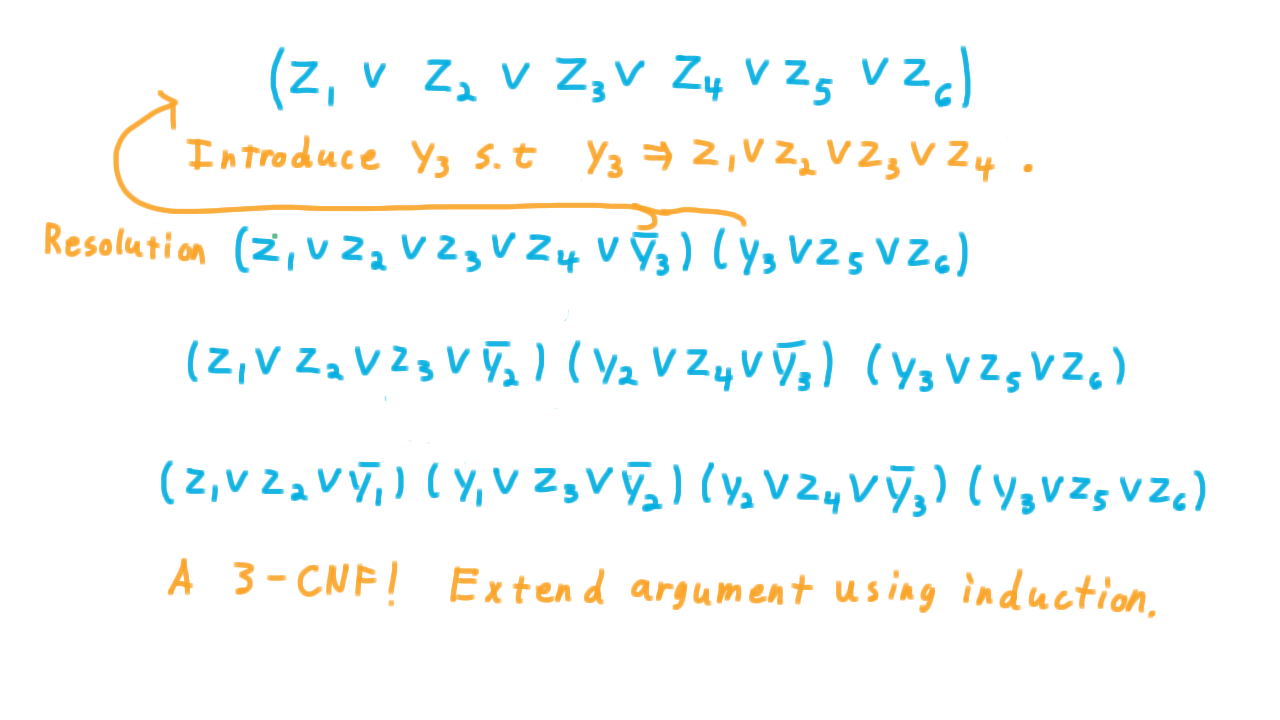
The example is for \(k=6,\) but an inductive argument will show that the argument works for any k greater than 3.

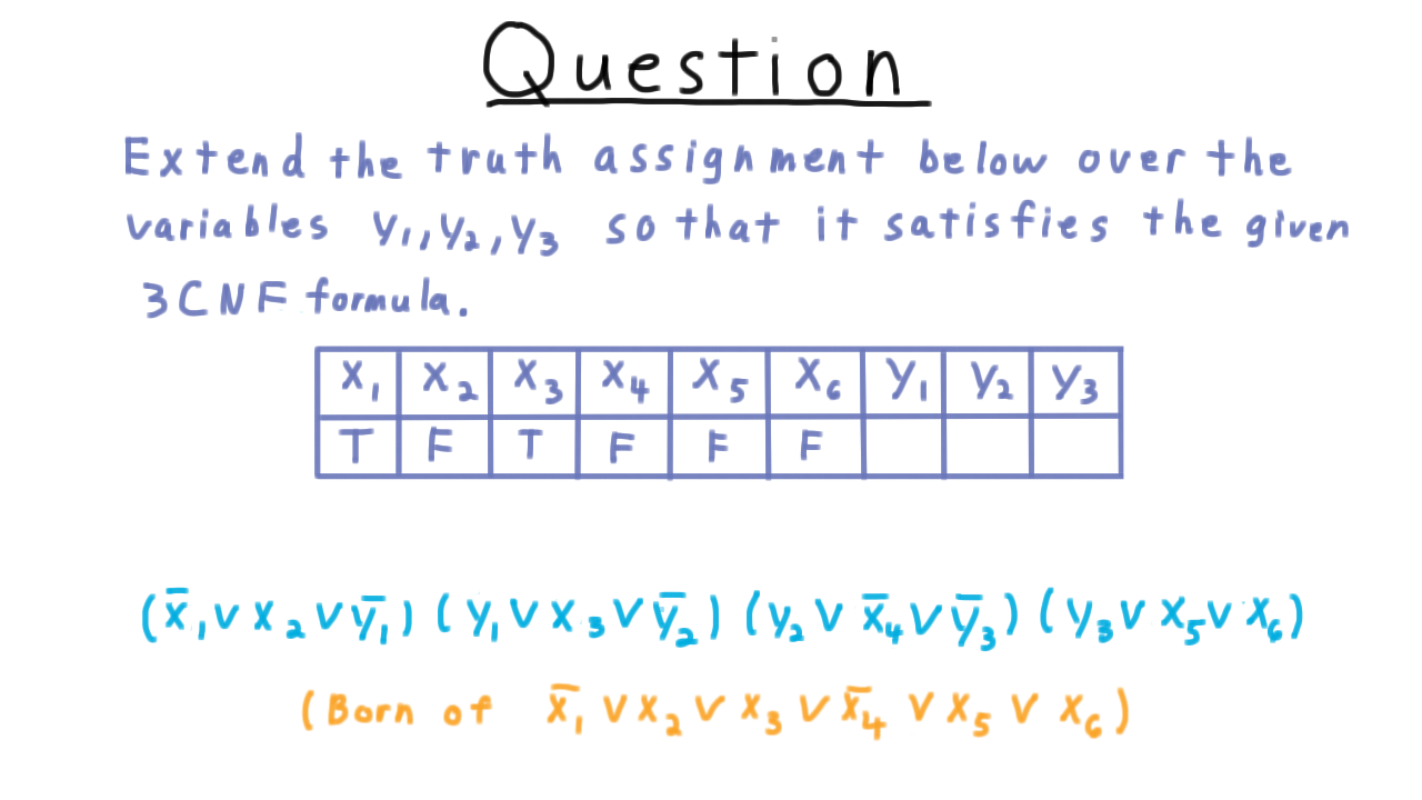
Extending A Truth Assignment - (Udacity)

Here is an exercise intended to help you solidify your understanding of the relationship between the original clause and the set of 3 clauses that the transformation produces. I want you to extend the truth assignment below so that it satisfies the given 3CNF formula. This one is the image of this clause here under the transformation that we’ve discussed.

CNF SAT - (Udacity, Youtube)

Recall that our original purpose was to find a transformation of the formula such that an truth assignment satisfied the original if and only if it could be extended to the transformed formula.

We’ve seen how to do this transformation for a single clause, and actually this is enough. We can just transform each clause individually introducing a new set of variables for each; all of the same argument about extending or restricting the truth assignment will hold.

Let’s illustrate what a transformation of multi-clause formula looks like with an example. Consider this formula here,

\[(z_{11} \vee z_{12}) \wedge (z_{21} \vee z_{22} \vee z_{23} \vee z_{24} \vee z_{25}) \]

where I’ve indexed the literals \(z\) with two indices now, the first referring to the clause it’s in and the second being its enumeration within the clause.

The first clause only has two literals, so we transform it into these two clauses with 3 literals by introducing a new variable \(y_{11}.\) It gets the first 1 because it was generated by the first clause.

We transform this second clause with 5 literals into these three clauses introducing the two new variables \(y_{21}\) and \(y_{22}\). Note that these are different from the variables used in the clauses generated by the the first original clause. Since all of these sets of variables are disjoint, we can assign them independently of each other and apply all the same arguments as we did to individual clauses. The results are shown below.

That’s how CNF can be reduced to 3CNF. This transformation runs in polynomial time, making the reduction polynomial.

We just reduced the problem of finding a satisfying to a CNF formula to the problem of finding a satisfying assignment to a 3CNF formula. At this point, it’s natural to ask, “can we go any further? Can we reduce this problem to a 2CNF?” Well no, not unless P=NP. There is a polynomial time algorithm for finding a satisfying a 2-CNF formula based on finding strongly connected components. Therefore, If we could reduce 3-CNF to 2CNF, then P=NP.

So 3CNF is as simple as the satisfiability question gets, and it admits some very clean and easy-to-visualize reductions that allow us to show that other problems are in NP. We’ll go over two of these: first, the reduction to independent set (or clique) and then to Subset Sum.

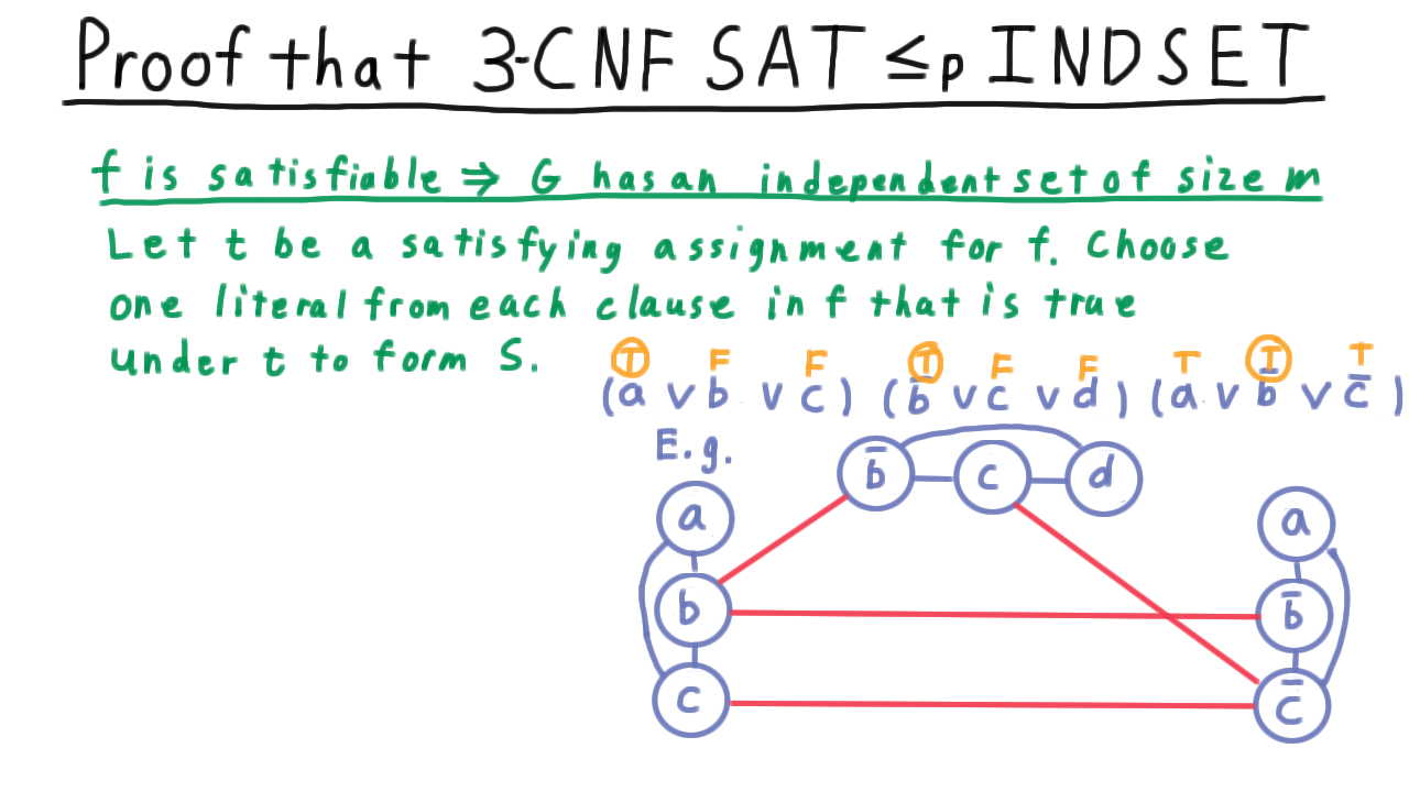
3CNF INDSET - (Udacity, Youtube)

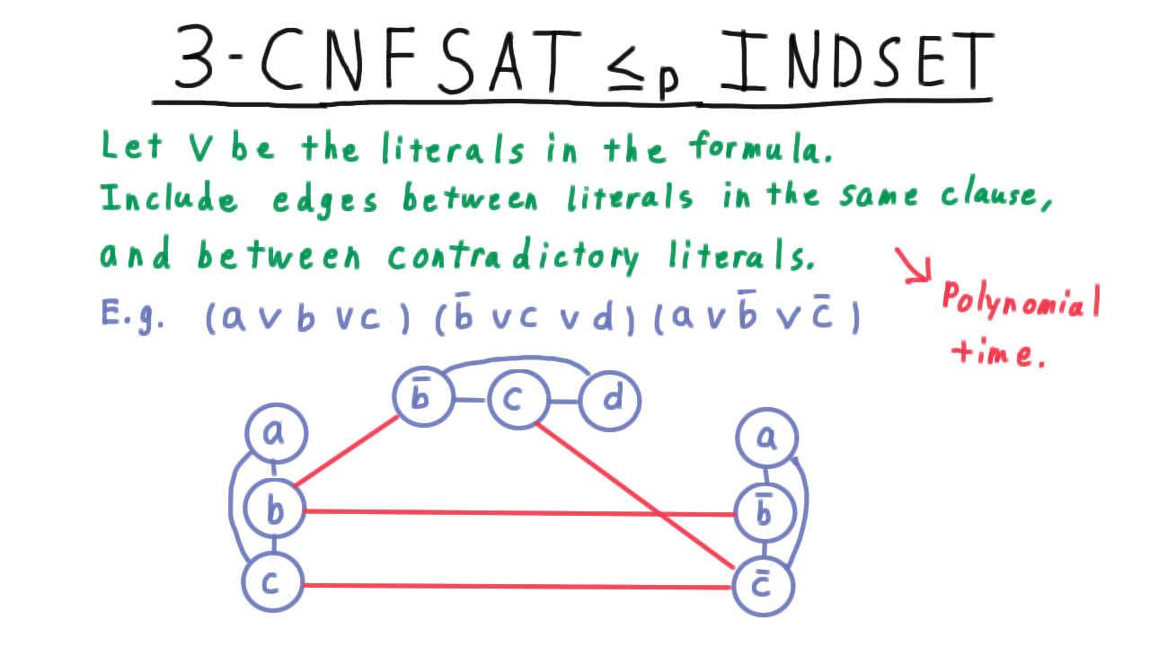
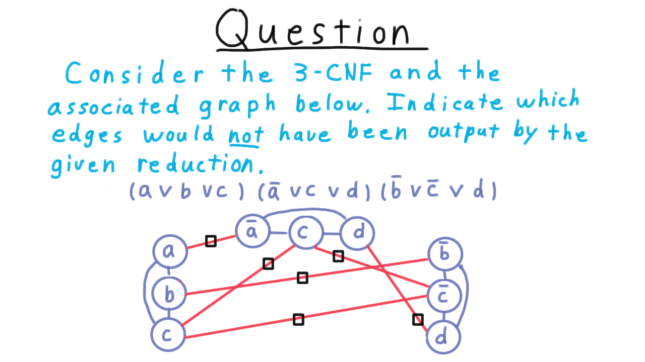
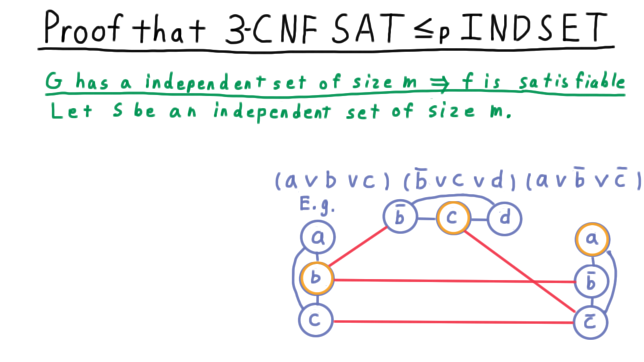
A the beginning of the lesson, we promised that we could link up these two chains and use the transitivity of reductions to show that Vertex Cover and Independent Set were NP-complete. We now turn to the last link in this chain and will reduce 3CNF-SAT to Independent Set. As we’ve already argued these problems are in NP, so that will complete the proofs.

Here then is the transformation, or reduction, we need to accomplish. The input is a 3CNF formula with m clauses, and we need to output a graph that has an independent set of size m if and only if the input is satisfiable.
We’ll illustrate on this example.

\[(a \vee b \vee c) \wedge (\overline{b} \vee c \vee d) \wedge (a \vee \overline{b} \vee \overline{c}) For each literal in the formula, we create a vertex in a graph. Then we add edges between all vertices that came from the same clause. We'll refer to these as the within-clause edges or simply the clause edges. Then we add edges between all literals that are contradictory. We'll refer to these as the between-clause edges or the contradiction edges.

The implementation of this transformation is simple enough to imagine, and I'll leave it to you to convince yourself that it can be done in polynomial time. ###Which Edges Don't Belong - (Udacity) Here is a question to make sure you understand the reduction just given. Consider the formula below and the associated graph. Indicate the edges would NOT have been output by the transformation just described. ###Proof that 3CNF INDSET - (Udacity, Youtube) Next, we are going to prove that the transformation just described does in fact reduce 3CNF Satisfiability to Independent set. We'll start by arguing that if \\(f\\) is satisfiable then the graph \\(G\\) that is output has an independent set of size \\(m,\\) the number of clauses in \\(f.\\) Let \]$t\[ be a satisfying assignment. In our example, let's take the one that makes \\(a\\) true, \\(b\\) false, \\(c\\) false and \\(d\\) false, and well set the complements accordingly. Then we choose one literal from each clause in the formula that true under the truth assignment to form our set S. Thus, in our example I might choose this the literals, as indicated by the circled T's in the figure below. Clearly, the size of the set is \\(m,\\) the number of clauses. Because the vertices comes from distinct clauses there can't be any within-clause edges, and because the truth assignment t doesn't contradict itself, there can't be an contradiction or between-clause edges either. Therefore, \\(S\\) must be an independent set. Let's prove the other direction next. If graph \\(G\\) output by the proposed reduction has an independent set of size \\(m,\\) then \\(f\\) is satisfiable. We start with an independent set of size \\(m\\) in the graph. Here, I have marked an independent set in our example graph. The fact that there can be no within-clause edges in \\(S\\) implies that the literals in \\(S\\) must come from distinct clauses. The fact that there can be no between-clause edges implies that the literals in \\(S\\) are non-contradictory. Therefore, any assignment consistent with the literals of \\(S\\) will satisfy \\(f.\\) Here, the choice of literals implies that \\(a,\\) \\(b,\\) and \\(c\\) all be true, but \\(d\\) can be set to be true or false, and we still have a satisfying assignment. So that completes the proof that Independent Set is as hard as 3CNF, and that completes the chain, \] \mbox{CNF } \leq_P \mbox{ 3-CNF } \leq_P \mbox{ Independent Set } \leq_P \mbox{ Vertex Cover },$$

showing that both Independent Set and Vertex Cover are NP-complete.

Next, we are going to branch out both in the tree here and in the types of arguments we’ll make by considering the subset sum problem.

Subset Sum - (Udacity, Youtube)

Before reducing 3CNF to Subset Sum, we have to define the Subset Sum problem first. We are given a multiset of \(\\{a_1, \ldots, a_m\\}\), where each element is a positive integer. A multiset, by the way, is just a set that that allows the same element to be included more than once. Thus, a set might contain three 5s, two 20s and just one 31, for example. We are also given a number \(k.\) The problem is to decide whether there is a subset of this multiset whose members add up to \(k.\)

One instance of this problem is partitioning, and I’ll use this particular example to illustrate.

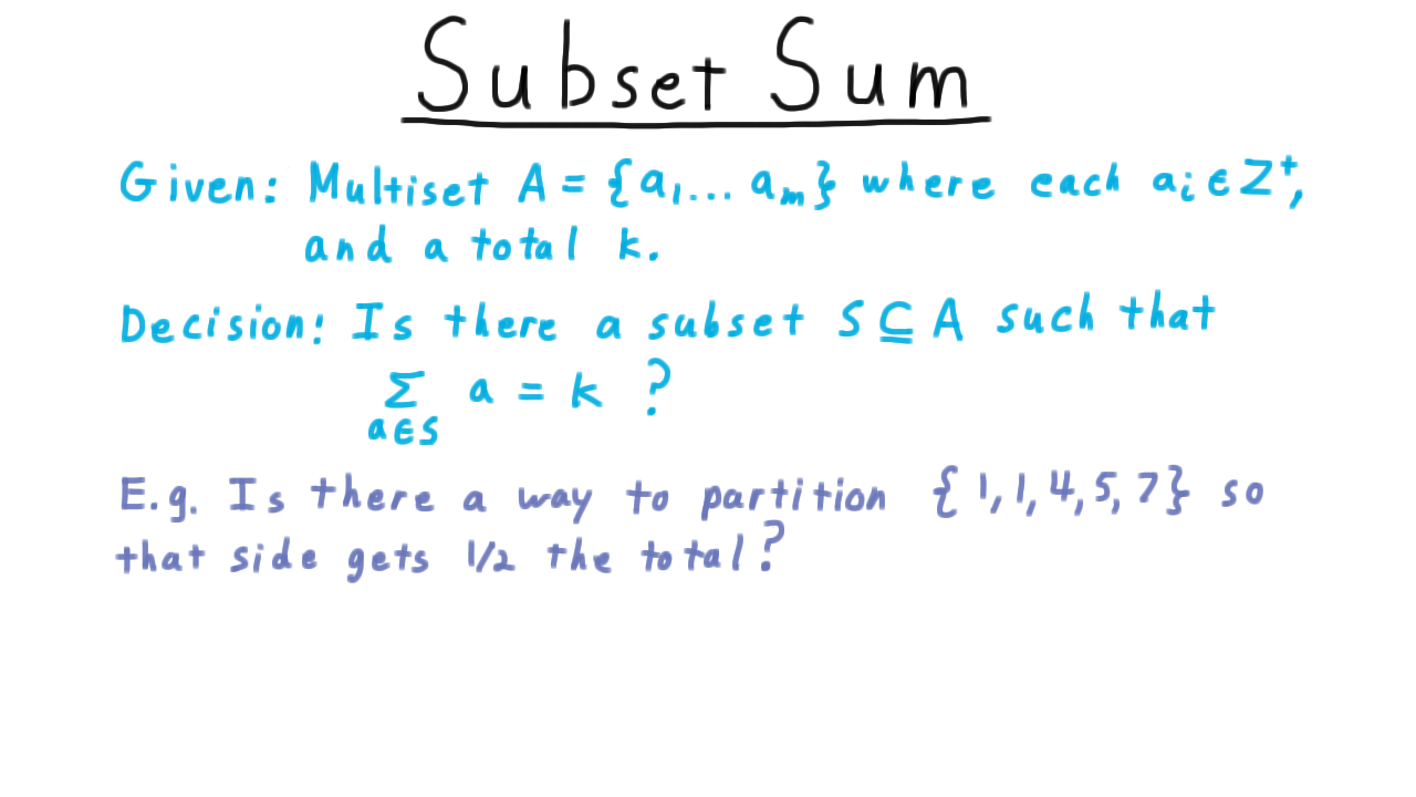
Imagine that you wanted to divide assets evenly between two parties–maybe we’re picking teams on the playground, trying to reach a divorce settlement, dividing spoils among the victors of war, or something of that nature. Then the question becomes, “Is there a way to partition a set so that things come out even, each side getting exactly 1/2?”

In this case, the total is 18, so we could choose \(k\) to be equal to 9 and then ask if there is a way to get a subset to sum to 9.
Indeed, there is. We can choose the two \(1\)s and the 7, and that will give us 9. Choosing 4 and 5 would work too, of course.

That’s the subset sum problem then. Note that the problem is in NP because given a subset, it takes polynomial time to add up the elements and see if the sum equals k. Finding the right subset, however, seems much harder. We don’t know of a way to do it that is necessarily faster than just trying all 2^m subsets.

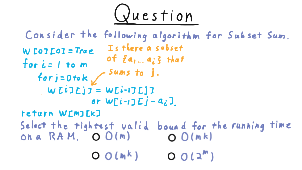
A Subset Sum Algorithm - (Udacity)

We are going to show that Subset Sum is NP-complete, but here is a simple algorithm that solves it. \(W\) is a two-dimensional array of booleans
and \(W[i][j]\) indicates whether there is a subset of the first \(i\) elements that sums to \(j.\) There are only two ways that this can be true:

• either there is a way to get \(j\) using only elements \(1\) through \(i-1,\)
• or there is a way to get \(j-a_i\) using the first \(i-1,\) and then we include \(a_i\) to get \(j.\)

For now, I just want you to give the the tightest valid bound on the running time for a Random Access Machine.

3 CNF Subset Sum - (Udacity, Youtube)

Here is the reduction of 3-CNF SAT to Subset Sum. We’ll illustrate the reduction with an example, because writing out the transformation in its full generality can get a little messy. Even with just an example, the motivation for the intermediate steps might not be clear at the time. It should all become clear at the end, however.

We’re going to create a table with columns for the variables and columns for the clauses. The rows of the table are going to be numbers in our subset, and we’ll have this column represent the ones place, this one the tens place, and so forth.

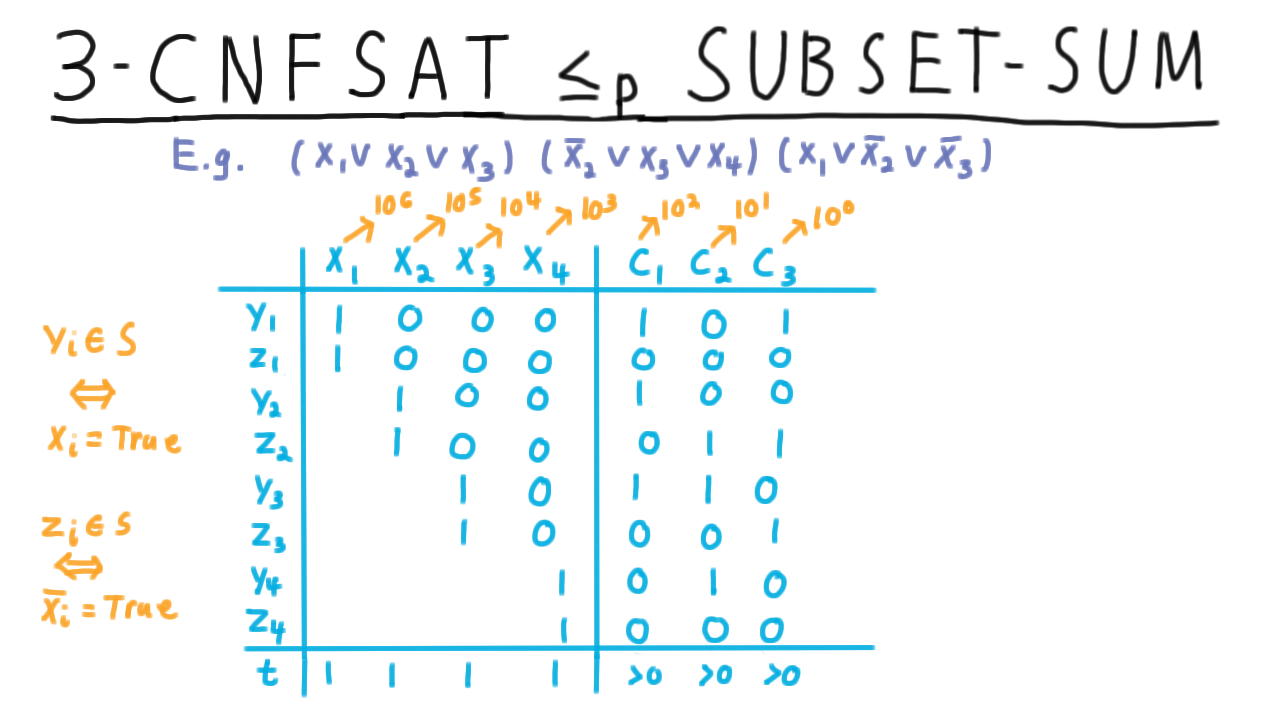
The collection of numbers will consist of two numbers for every variable in the formula: one that we include when t(x_i) is true–we’ll notate those with y– and another that we include when it is false–we’ll notate those with z.

In the end, we want to include either \(y_i\) or \(z_i\) for every \(i,\) since we have to assign the variable \(x_i\) one way or the other. To get a satisfying assignment, we also have to satisfy each clause, so we’ll want the numbers \(y_i\) and \(z_i\) to reflect which clauses are satisfied as well. The number \(y_1\) sets \(x_1\) to true, so we put a 1 in that column to indicate that choosing \(y_1\) means assigning \(x_1\). Since this assigns \(x_1\) to be true, it also means satisfying clauses 1 and 3 in our example.

Choosing \(z_1\) also would assign the variable \(x_1\) a value, but it wouldn’t satisfy any clauses. Therefore, that row is the same as for \(y_1\) except in the clause columns where are all set to zero.

We do the analogous procedure for \(y_2\) and \(z_2\): the literal \(x_2\) appears in clause 1, and the literal \(\overline{x_2}\) appears in clauses 2 and 3. We can do the same for variables \(x_3\) and \(x_4.\) These then are the numbers that we want to include in our set A.

It remains to choose our desired total \(k.\) For each of these variable columns the desired total is exactly 1. We assign each variable one way or the other. For these clause columns, however, the total just has to be greater than 0. We just need one literal in the clause to be true in order for the clause to be satisfied. Unfortunately, that doesn’t yield a specific \(k\) that we need to sum to.

The trick is to add more numbers to the table.

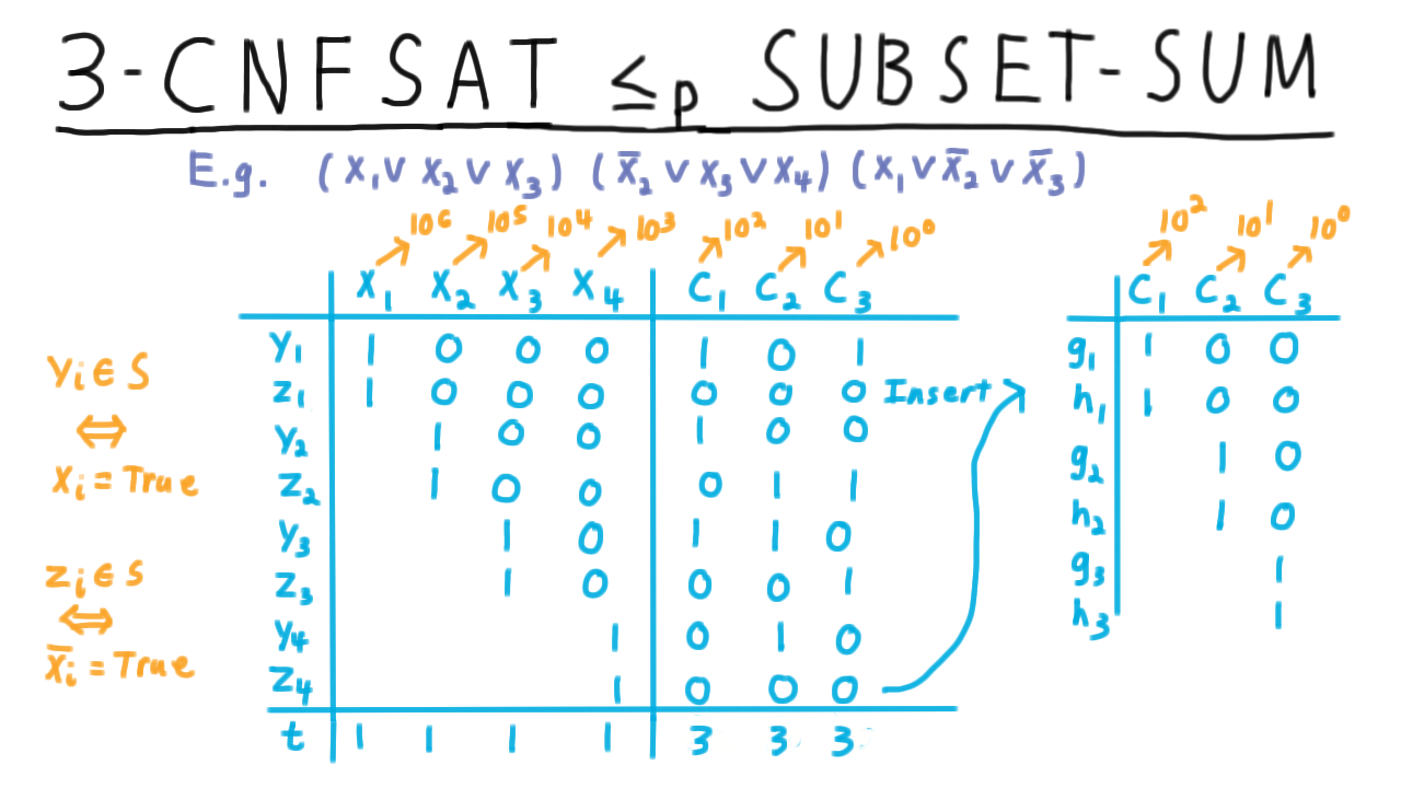
These all have zeros in the places corresponding to the variables, and exactly one 1 in a column for a clause. Each clause \(j\) gets two numbers that have a 1 in the \(j\)th column. We’ll call them \(g_j\) and \(h_j.\)
This allows us to see the desired number to be 3 in the clause columns. Given a satisfying assignment, the corresponding choice of \(y\) and \(z\) numbers will have at least a 1 in all the clause columns but no more than 3. All the \(1\)s and \(2\)s can be boosted up by including the \(g\) and \(h\) numbers. Note that if some clause is unsatisfied, then include the \(g\) and \(h\) numbers isn’t enough to bring the total to 3 because there are only two of them.

That’s the construction. For each variable the set of number to choose from includes two numbers \(y\) and \(z\) which will correspond to the truth setting, and for each clause it includes \(g\) and \(h\) so that we can boost up the total in the clause column to three where needed.
This construction just involves a few for-loops, so it’s easy to see that the construction of the set of numbers is polynomial time.

Proof that 3CNF SUBSET SUM - (Udacity, Youtube)

Next, we prove that this reduction works. Let \(f\) be a 3CNF formula with \(n\) variables and \(m\) clauses. Let \(A\) be the multiset over the positive integers and \(k\) be the total number output by the transformation.

First, we show that if \(f\) is satisfiable then there is a subset of \(A\) summing to \(k.\) Let \(t\) be the satisfying assignment. Then we include \(y_i\) in \(S\) if \(x_i\) is true under t, and we’ll include \(z_i\) otherwise. As for the \(g\) and \(h\) families of numbers, if there are fewer than three literals of clause j satisfied under \(t,\) then include \(g_j.\) If there are a fewer than 2, then include \(h_j\) as well. In total, the sum of these numbers must be equal to \(k.\)

In the other direction, we argue that if there is a subset of \(A\) summing to \(k,\) then there is a satisfying assignment. Suppose that \(S\) is a subset of \(A\) summing to \(k.\) Then the impossibility of any “carrying” of the digits in any sum implies that exactly 1 of \(y_i\) or \(z_i\) must have been set to true. Therefore, we can define a truth assignment \(t\) where \(t(x_i)\) is true if \(y_i\) is included in \(S\) and false otherwise. This must satisfy every clause; otherwise, there would be no way that the total in the clause places would be 3.

Altogether, we’ve seen that Subset Sum in NP and we can reduce 3-CNF SAT an NP-complete problem to it, so Subset Sum must be NP-complete.

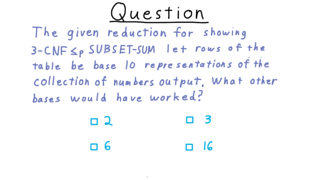
Other Bases - (Udacity)

Here is an exercise to encourage you to consider carefully the reduction just given. We interpreted the rows of the table we constructed as the base 10 representation of the collection of numbers that the reduction output. What other bases would have worked as well? Check all that apply.

Conclusion - (Udacity, Youtube)

So far, we’ve built up a healthy collection of NP-complete complete problems, but given that there are thousands of problems know to be NP-complete, we’ve only scratched the surface of what is known. In fact, we haven’t even come close to Karp’s mark of 21 problems from his 1972 paper.
If you want to go on and extend the set of problems that you can prove to be NP-complete, you might consider reducing subset sum to the Knapsack problem, where one has a fixed capacity for carrying stuff and want to pack the largest subset of items that will fit.
Another classic problem is that of the Traveling Salesman. He has a list of cities that he wants to visit and, he wants to know the order that will minimize the distance that he has to travel. One can prove that this problem is NP-complete by first reducing Vertex Cover to the Hamiltonian Cycle problem—which asks if there is a cycle in a graph that visits each vertex exactly once—and then Hamiltonian Cycle to Traveling Salesman.
Another classic problem that is used to prove other problems are NP-complete is 3D-matching. 2D matching can be thought of as the problem making as many compatible couples as possible from a set of people. 3D matching extends this problem by further matching them with a home that they would enjoy living in together.

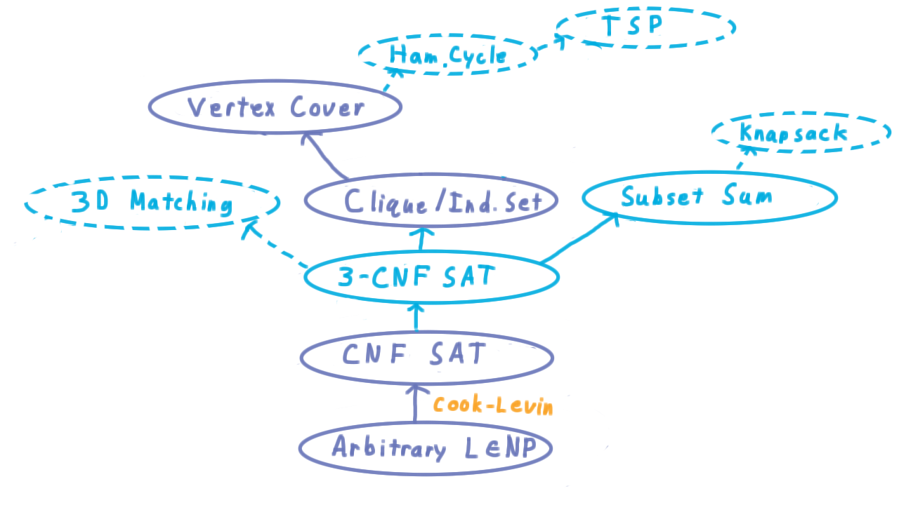
Of course, there are many others. The point of this lesson, however, is not so that you can produce the needed chain of reductions for every problem known to be NP-complete. Rather, it is to give you a sense for what these arguments look like and how you might go about making such an argument for a problem that is of particular interest to you.

The reductions we’ve given as examples are a fine start, but if you want to go further in understanding how to use complexity to understand real-world problems, take a look at the classic text by Garey and Johnson on Computers and Intractability. Even though it is from the same decade as the original Cook-Levin result and Karp’s list of 21 NP-complete problems, it is still one of the best. As Lance, says “a good computer scientist shouldn’t leave home without it.”