Computability, Complexity, and Algorithms
Charles Brubaker and Lance Fortnow
Computability, Complexity, and Algorithms
Charles Brubaker and Lance Fortnow
NP-Completeness - (Udacity)
Introduction - (Udacity, Youtube)
This lecture covers the theory of NP-completeness, the idea that there are some problems in NP so general and so expressive that they capture all of the challenges of solving any problem in NP in polynomial time. These problems provide important insight into the structure of P and NP, and form the basis for the best arguments we have for the intractability of many important real-world problems.
The Hardest Problems in NP - (Udacity, Youtube)
With our previous discussion of the classes P and NP in mind, you can visualize the classes P and NP like this.
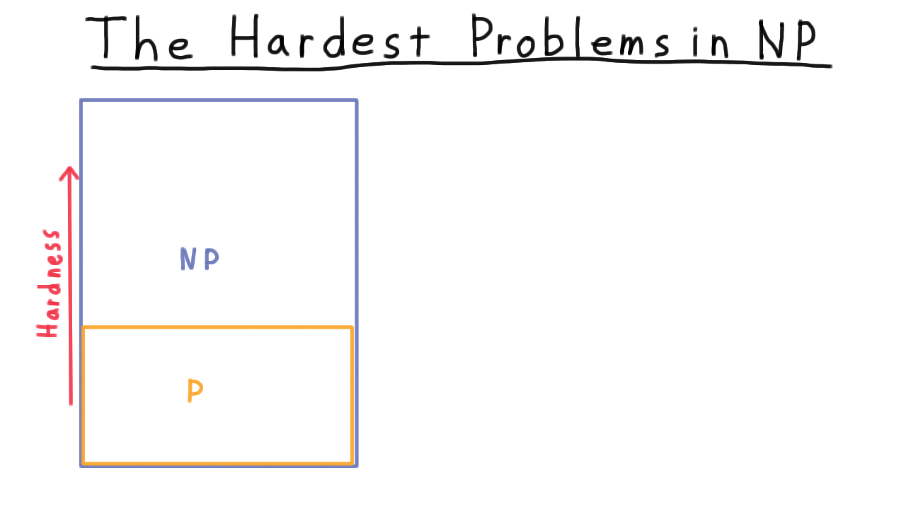
Clearly, P is contained inside of NP, and we are pretty sure that this containment is strict. That is to say that there are some problems in NP but not in P, where the answer can be verified efficiently, but it can’t be found efficiently. In this picture then, you can imagine the harder problems being at the top.
Now, suppose that you encounter some problem where you know how to verify the answer, but where you think that finding an answer is intractable. Unfortunately, your boss or maybe your advisor doesn’t agree with you and keeps asking for an efficient solution.
How would you go about showing that the problem is in fact intractable? One idea is to show that the problem is not in P. That would indeed show that it is not tractable, but it would do much more. It would show that P is not equal to NP. You would be famous. As we talked about in the last lecture, whether P is equal to NP is one of the great open questions in mathematics. Let’s rule option out. I don’t want to discourage you from trying to prove this theorem necessarily. You just should know what you are getting into.
Another possible solution is to show that if you could solve your problem efficiently then it would be possible to solve another problem efficiently, one that is generally considered to be hard. If you were working in the 1970’s you might have shown that a polynomial solution to your problem would have yielded a polynomial solution to linear programming. Therefore, your problem must be at least as hard a linear programming. The trouble with this approach is that it was later shown that linear programming actually was polynomially solvable. Hence, the fact your problem is as hard as linear programming doesn’t mean much anymore. The class P swallowed linear programming. Why couldn’t it swallow your program as well? This type of argument isn’t worthless, but it’s not as convincing as it might be.
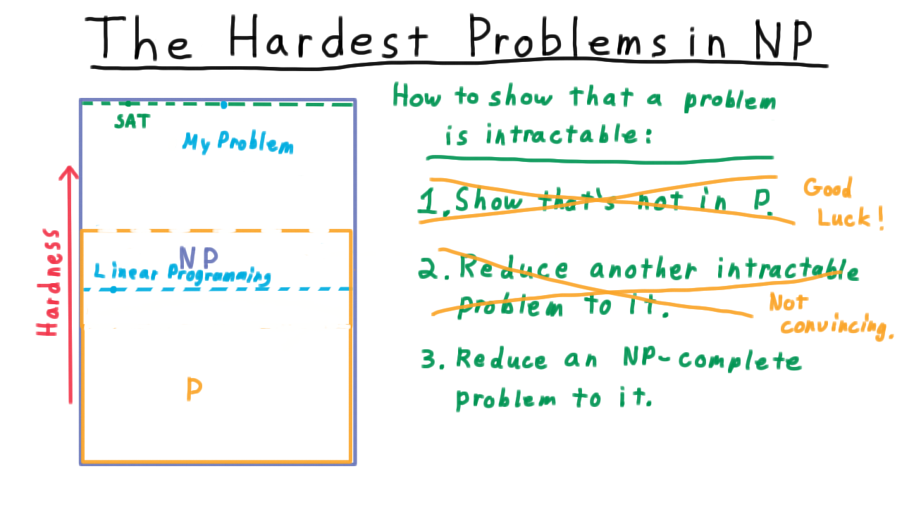
It would be much better to reduce your problem to a problem that we knew was one of the hardest in the class NP, so hard that if the class P were to swallow it would have to have swallowed all of NP. In other words, we would have to move the P borderline all the way to the top. Such a problem would have to be NP-complete, meaning that we can reduce every language in NP to it. Remarkable as it may seem, it turns out that there are lots of such languages–satisfiability being the first for which this was proved. In other words, we know that it has to be at the top of this image. Turning back to how to show that your problem is intractable, short of proving that P is not equal to NP, the best we can do is to reduce an NP-complete problem like SAT to your problem. Then, your problem would be NP-Complete too, and the only way your problem could be polynomially solvable is if everything in NP is.
There are two parts to this argument.
- The first is the idea of a reduction. We’ve seen reductions before in the context of computability. Here the reductions will not only have to be computable but computable in polynomial time. This idea will occupy the first half of the lesson.
- The second half will consider this idea of NP-completeness and we will go over the famous Cook-Levin theorem which show that boolean satisfiability is NP-complete
Polynomial Reductions - (Udacity, Youtube)
Now for the formal definition of a polynomial reduction. This should feel very similar to the reductions that we considered when were talking about computability.
A language \(A\) is polynomially reducible to language \(B\) (\(A \leq_P B\)) if there is a polynomial-time computable function \(f\) where for every string w,
\[w \in A \Longleftrightarrow f(w) \in B.\]
The key difference from before is that we have now required that the function be computable in polynomial time, not just that it be computable. We will also say that \(f\) is a polynomial time reduction of \(A\) to \(B.\)
Here is key implication of there being a polynomial reduction of one language to another. Let’s suppose that I want to be able to know whether a string \(x\) is in the language \(A\), and suppose also that there exists a polynomial time decider \(M\) for the language \(B.\)
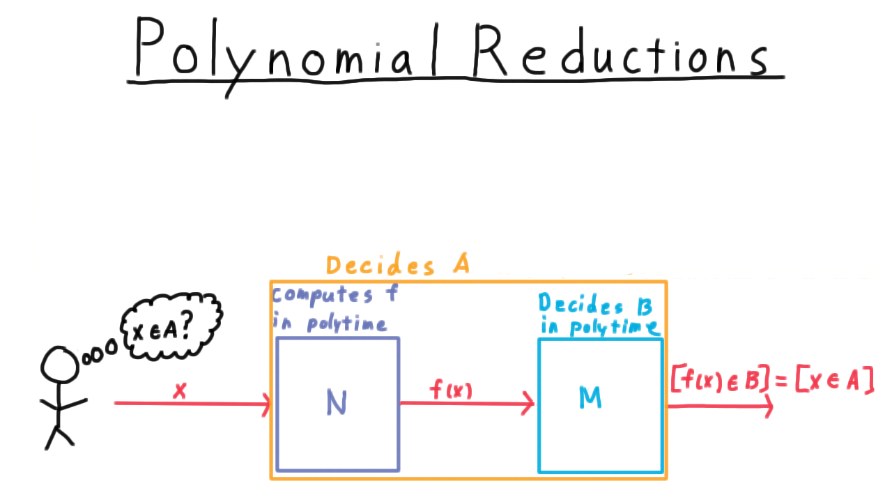
Then, all I need to do is take the machine or program that computes this function–let’s call it \(N\)–
and feed my string \(x\) into it, and then feed that output into \(M.\) The machine \(M\) will tell me if \(f(x)\) is in \(B.\) By the definition of a reduction, this also tells me whether \(x\) is in \(A,\) which is exactly what I wanted to know. I just had to change my problem into one encoded by the language \(B\) and then I could use \(B\)’s decider.
Therefore, the composition of \(M\) with \(N\) is a decider for \(A\) by all the same arguments we used in the context of computability. But is it a polynomial decider?
Running Time of Composition - (Udacity)
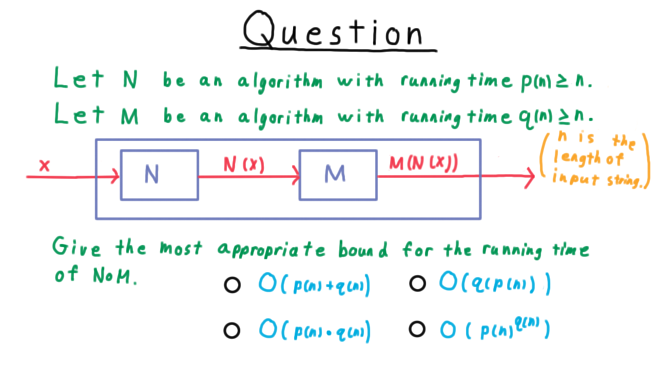
We just found ourselves considering the running time of the composition of two Turing machines. Think carefully, and give the most appropriate bound for the running time of the composition of \(M\) which runs in time \(q\) with \(N\) which runs in time \(p.\) You can assume that both \(N\) and \(M\) at least read all of their input.
Polynomial Reductions Part 2 - (Udacity, Youtube)
We just argued that if \(N\) is polynomial and we take its output and feed that into \(M\) which is also polynomial in its input size, then the resulting composition of \(M\) with \(N\) is also polynomial. Therefore, we can add “in polytime” to our claim in the figure.

By this argument, we’ve proved the following important theorem.
If A is polynomially reducible to B, and B is in P, then A must be in P.
Just convert the input string to prepare it for the decider for \(B,\) and return what the decider for \(B\) says.
What Do Reductions Imply - (Udacity)
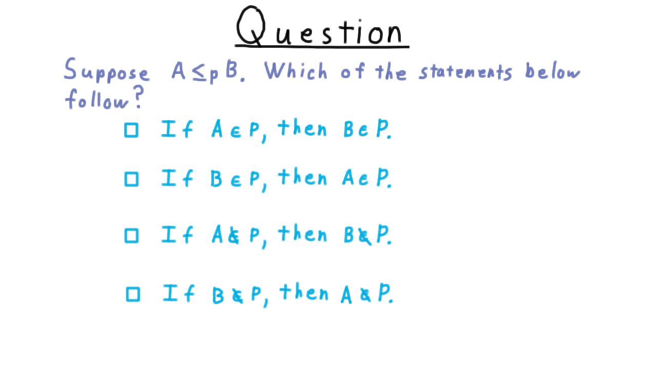
Here is a question to test your understanding of the implications of the existence of a polynomial reduction. Suppose that \(A\) reduces to \(B,\) which of the statements below follow?
Independent Set - (Udacity, Youtube)
To illustrate the idea of a polynomial reduction, we’re going to reduce the problem of finding a Independent Set in a graph to that of finding a Vertex Cover. In the next lesson, we going to argue that if P is not equal to NP, then Independent Set is not in P, so Vertex Cover can’t be either. But that’s getting ahead of ourselves. For the benefit of those not already familiar with these problems, we will state them briefly.
First, we’ll consider the independent set problem and see how it is equivalent to the Clique problem that we talked about when we introduced the class NP.
Given a graph, a subset \(S\) of the vertices is an independent set if there are no edges between vertices in \(S.\)
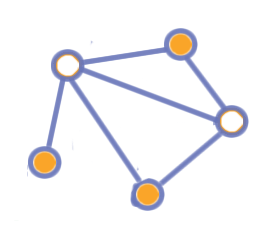
These two vertices here do not form an independent set because there is an edge between them.

However, these three vertices do form an independent set because there are no edges between them.
Clearly, each individual vertex forms an independent set, since there isn’t another vertex in the set for it to have an edge with, and the more vertices we add the harder it is to find new ones to add. Finding a maximum independent set, therefore, is the interesting question. Phrased as a decision problem, the question becomes “given a graph G, is there an independent set of size \(k\)?”
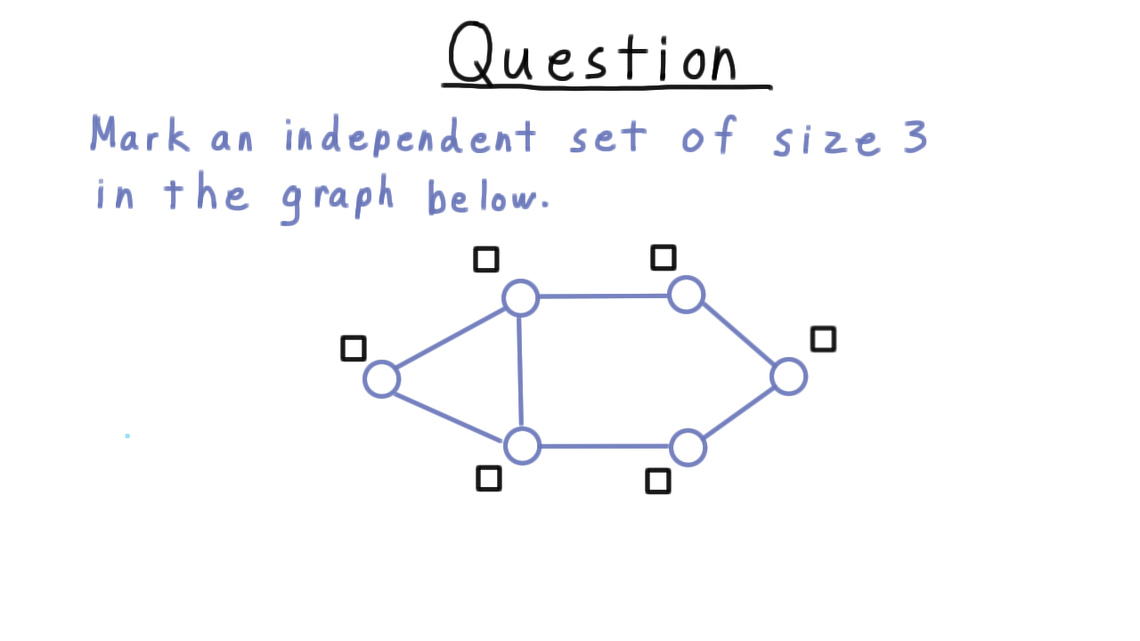
Find an Independent Set - (Udacity)
In order to understand the reduction, it is critical that you understand the independent set problem, so here is a quick question to test your understanding. Mark an independent set of size 3.
Vertex Cover - (Udacity, Youtube)
Now let’s define the other problem that will be part of our example reduction, Vertex Cover.
Given a graph G, a subset \(S\) of the vertices forms a vertex cover if every edge is incident on \(S\) (i.e. has one part in \(S\)).
To illustrate, consider this graph here. These three shaded vertices do not form a vertex cover.
On the other hand, the two vertices do form a vertex cover because every edge is incident on one of these two.
Clearly, the set of all vertices is a vertex cover, so the interesting question is how small a vertex cover can we get. Phrased as a decision question where we are give a graph G, it becomes “Is there a vertex cover of size \(k\)?”
Note that this problem is in NP. It’s easy enough to check whether a subset of vertices is of size \(k\) and whether it covers all the edges.
Find a Vertex Cover - (Udacity)
Going forward, it will be very important to understand this vertex cover problem, so we’ll do a quick exercise to give you a chance to test your understanding. Mark a vertex cover of size 3 in the graph below.

Vertex Cover = Ind Set - (Udacity, Youtube)
Having defined the Independent Set and Vertex Cover problems, we will now show that Vertex Cover is as hard as Independent set. In general, finding a reduction can be very difficult. Sometimes, however, it can as simple as playing around with a definition.

Notice that both in these examples shown here and in the exercises, the set of vertices used in the vertex cover was the complement of the vertices used the independent set. Let’s see if we can explain this.
- The set S is an independent set if there are no edges within S. By within, I mean that both endpoints are in S.
- That’s equivalent to saying that every edge is not within S…or that every edge is incident on \(V - S.\)
- But that just says that \(V-S\) is a vertex cover! The complement of an independent set was always a vertex cover and vice-versa.
Thus, we have the observation that
A subset of vertices \(S\) is an independent set if and only if \(V-S\) is a vertex cover.
As a corollary then,
A graph G has an independent of size at least \(k\) if and only if it contains a vertex cover of size at most size \(V - k\).
The reduction is therefore fantastically simple: Given a graph G and a number \(k,\) just change \(k\) into \(V-k.\)
Transitivity of Reducibility - (Udacity, Youtube)
The polynomial reducibility of one problem to another is a relation, much like the at most relation that you seen since elementary school. While it doesn’t have ALL the same properties, it does have the important property of transitivity. For example, we’ve seen how independent set is reducible to vertex cover, and I claim that vertex cover is reducible to Hamiltonian Path, a problem closely related to Traveling Salesman. From these facts it follows that independent set is reducible to Hamiltonian Path.
Let’s take a look at the proof of this theorem. Let \(M\) be the program that computes the function that reduces \(A\) to \(B,\) and let \(N\) be the program that computes the function that reduces \(B\) to \(C.\) To turn an instance of the problem \(A\) into an instance of the problem \(C,\) we just pass it through \(M\) and then pass that result through \(N.\)
This whole process can be thought of as another computable function \(R.\)
Note that like \(M\) and \(N,\) \(R\) is polynomial time. I’ll ask you to help me show why in a minute.
Thus, \(x\) is in \(A\) if and only if \(M(x)\) is in \(B\)–because \(M\) implements the reduction– and \(M(x)\) is in \(B\) if and only if \(N(M(x))\) is in C – because \(N\) implements that reduction. The composition of \(N\) and \(M\) is the reduction \(R,\) so overall we have that \(x\) is in \(A\) if and only if \(R(x)\) is in \(C,\) just as we wanted.
NP Completeness - (Udacity, Youtube)
If you have followed everything in the lesson so far, then you are ready to understand NP-completeness, an idea behind some of the most fascinating structure in the P vs NP question. You may have heard optimists say that we are only one algorithm away proving that P is equal to NP. What they mean is that if we could solve just one NP-complete problem in polynomial time, then we could solve then all in polynomial time. Here is why.
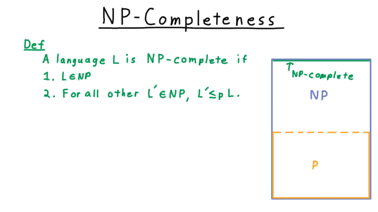
Formally, we say
A language \(L\) is NP-complete if \(L\) is in NP and if every other language in NP can be reduced to it in polynomial time.
Recalling our picture of P and NP from the beginning of the lesson the NP-complete problems were at the top of NP, and we called them the hardest problems in NP. We can’t have anything higher that’s still in NP, because if it’s in NP, then in can be reduced to an NP-complete problem. Also, if any one NP-complete problem were shown to be in P, then P would extend up and swallow all of NP.
It’s not immediately obvious that an NP-complete problem even exists, but it turns out that there are lots of them and in fact they seem to occur more often in practice than problems than problems in the intermediate zone, which are not NP-complete and so far have not been proved to be in P either.
Historically, the first natural problem to be proved to be NP-Complete is called Boolean formula satisfiability or SAT for short.
SAT is NP-Complete
This was shown to be NP-Complete by Stephen Cook in 1971 and independently by Leonid Levin in the Soviet Union around the same time. The fact that this problem is NP-complete is extremely powerful, because once you have one NP-Complete problem, you just need to reduce it to other problems in NP to show that they too are NP-complete. Thus, much of the theory of complexity can be said to rest on this theorem. This is the high point of our study of complexity.
CNF Satisfiability - (Udacity, Youtube)
For our purposes, we won’t have to work with the most general satisfiability problem. Rather, we can restrict ourselves to a simpler case where the boolean formula has a particular structure called conjunctive normal form, or CNF, like this one here.

First, consider the operators. The \(\vee\) indicates a logical OR, the \(\wedge\) indicates a logical AND, and the bar over top \(\overline{\cdot}\) indicates logical NOT.
For one of these formulas, we first need a collection of variables, \(x,y,z\) for this example. These variables appear in the formula as literals. A literal can be either a variable or the variable’s negation. For example, the \(x\), or \(\overline{y}\), etc.
At the next higher level, we have clauses, which are disjunctions of literals. You could also say a logical OR of literals. One clause is what lies inside of a parentheses pair.
Finally, we have the formula as a whole, which is a conjunction of clauses. That is to say, all the clauses get ANDed together.
Thus, this whole formula is in conjunctive normal form. In general, there can be more than two clauses that get ANDed together. That covers the terms we’ll use for the structure of a CNF formula.
As for satisfiability itself, we say that
A boolean formula is satisfiable if there is a truth assignment for the formula, a way of assigning the variables true and false such that the formula evaluates to true.
The CNF-satisfiability problem is: given a CNF formula, determine if that formula has a satisfying assignment.
Clearly, this problem is in NP since given a truth assignment, it is takes time polynomial in the number of literals to evaluate the formula. Thus, we have accomplished the first part of showing that satisfiability in NP-complete. The other part, showing that every problem in NP is polynomial-time reducible to it, will be considerably more difficult.
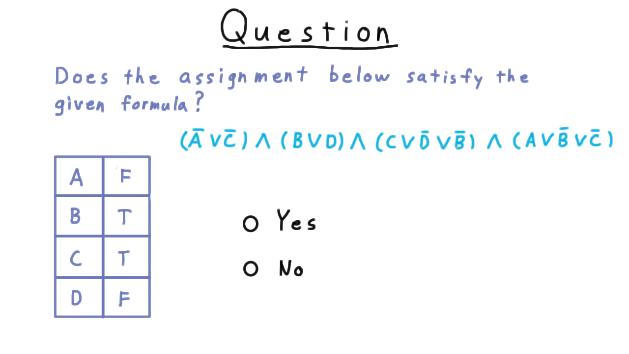
Does it Satisfy - (Udacity)
To check your understanding of boolean expressions, I want you to say whether the given assignment satisfies this formula.
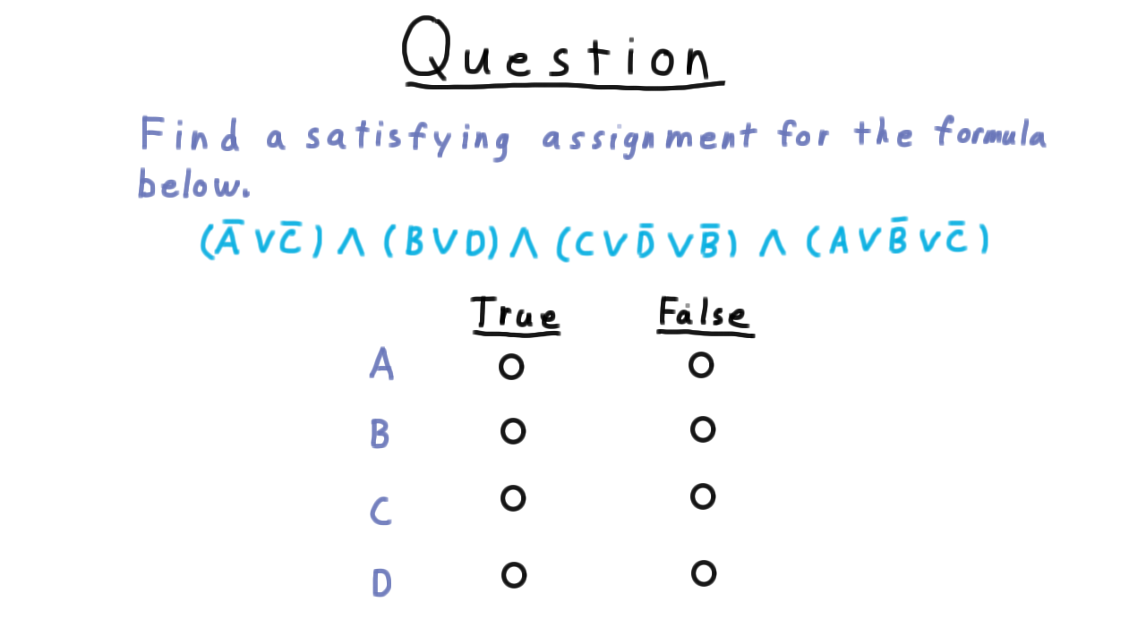
Find a Satisfying Assignment - (Udacity)
Just because one particular true assignment doesn’t satisfy a boolean formula doesn’t mean that there isn’t a satisfying assignment. See if you can find one for this formula. Unless you are a good guesser, this will take longer than just testing whether a given assignment satisfies the formula.
Cook Levin - (Udacity, Youtube)
Now that we’ve understood the satisfiability problem, we are ready to tackle the Cook-Levin theorem. Remember that we have to turn any problem in NP into an instance of SAT, so it’s natural to start with the thing that we know all problems in NP have in common: there is a nondeterministic machine that decides them in polynomial time. That’s the definition after all.
Therefore, let \(L\) be an arbitrary language in NP and let \(M\) be a nondeterministic Turing machine that decides \(L\) in time \(p(n),\) where \(p\) is bounded above by some polynomial.
An accepting computation, or sequence of configurations, for the machine M can be represented in a tableau like this one here.
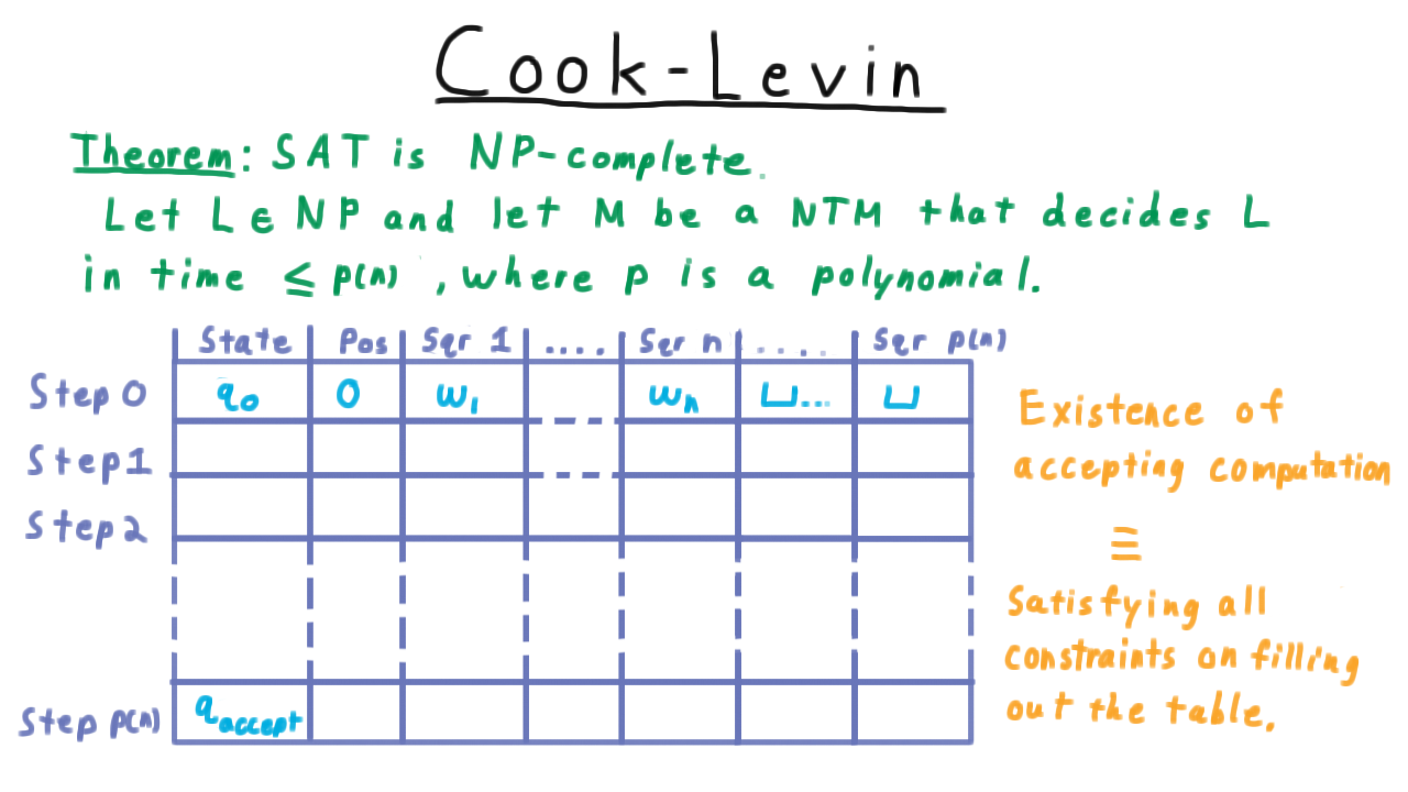
Each configuration in the sequence is represented by a row, where we have one column for the state, one for the head position and then columns for each of the values of the first \(p(n)\) squares of the tape. Note that no other squares can written to because there just isn’t time to move the head that far in only \(p(n)\) steps.
Of course, the first row must represent the initial configuration and the last one must be in an accepting state in order for the overall computation to be accepting.
Note that it’s possible that the machine will enter an accepting state before step \(p(n),\) but we can just stipulate that when this happens all the rest of the rows in the table have the same values. This is like having the accept state always transition to itself. The Cook-Levin theorem them consists of arguing that the existence of an accepting computation is equivalent to being able to satisfy a CNF formula that captures all the rules for filling out this table.
The Variables - (Udacity, Youtube)
Before doing anything else, we first need to capture the values in the tableau with a collection of boolean variables. We’ll start with the state column.

We let \(Q_{ik}\) represent whether after step \(i\), the state is \(q_k.\) Similarly, for the position column, we define \(H_{ij}\) to represent whether the head is over square j after step i. Lastly, for the tape contents, we define \(S_{ijk}\) to represent whether after step \(i,\) the square \(j\) contains the \(k\)th symbol of the tape alphabet.
Note that as we’ve defined these variables, there are many truth assignments that are simply nonsensical. For instance, every one of these \(Q\) variables could be assigned a value of True, but in a given configuration sequence the Turing machine can’t be in all states at all times. Similarly, we can’t assign them to be all False; the machine has to be in some state at each time step. We have the same problems with the head position variables and the variables for the squares of the tape.
All of this is okay. For now, we just need a way to make sure that any accepting configuration sequence has a corresponding truth assignment, and indeed it must. For any way of filling out the tableau, the corresponding truth assignment is uniquely defined by these meanings. It is the job of the boolean formula to rule out truth assignments that don’t correspond to valid accepting computations.
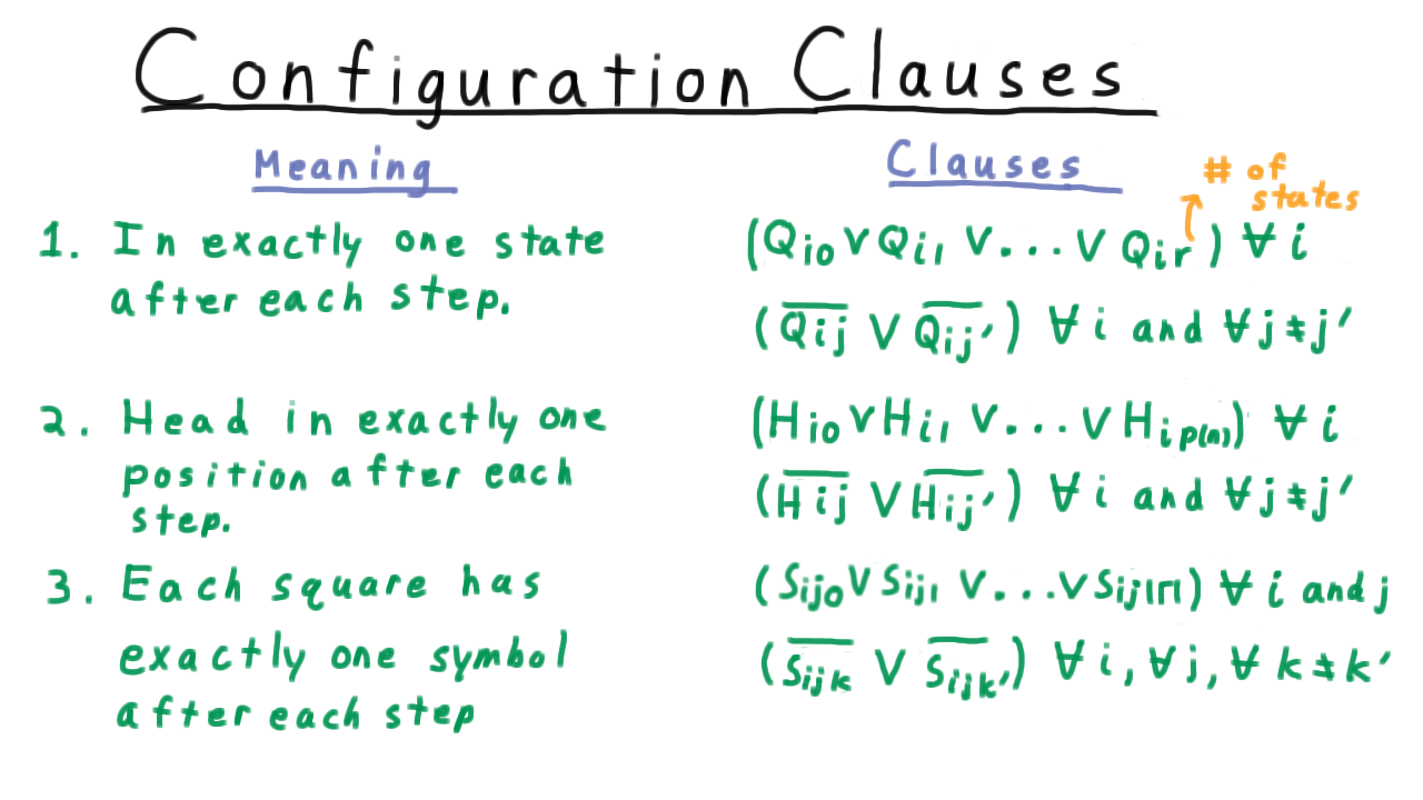
Configuration Clauses - (Udacity, Youtube)
Having defined the variables, we are now ready to move onto building the boolean formula. We are going to start with the clauses needed so that given a satisfying assignment it’s clear how to fill out the table. Never mind for now about whether the corresponding sequence is has valid transitions. For now, we just want the individual configurations to be well-defined.
First, we have to enforce that at each step the machine is in some state.
Hence for all \(i,\) at least one of the state variables for step \(i\) has to be true.
\[(Q_{i0} \vee Q_{i1} \vee \ldots \vee Q_{ir})\; \forall i\]
Note that \(r\) denotes the number of states here. In this context, it is just a constant. (The input to our reduction is the string that we need to transform into a boolean formula, not the Turing Machine description).
The machine also can’t be in two states at once, so we need to enforce that constraint as well by saying that for every pair of state variable for a give time step, one of the two has to be false.
\[(\overline{Q_{ij}} \vee \overline{Q_{ij'}}) \; \forall i, j\neq j'\]
Together these sets of clauses enforce that the machine corresponding to a satisfying truth assignment is in exactly one state after each step.
For the position of the head, we have a similar set of clauses. The head has to be over some square on the tape, but it can’t be in two places.
\[(H_{i0} \vee H_{i1} \vee \ldots \vee H_{ip(n)})\; \forall i\]
\[(\overline{H_{ij}} \vee \overline{H_{ij'}}) \; \forall i, j\neq j'\]
Lastly, each square on the tape has to have exactly one symbol. Thus, for all steps \(i\) and square \(j\), there has to be some symbol on the square, but there can’t be two.
\[(\overline{S_{ijk}} \vee \overline{S_{ijk'}}) \; \forall i, k\neq k'\]
So far, we have the clauses
The other clauses related to individual configurations come from the start and end states.
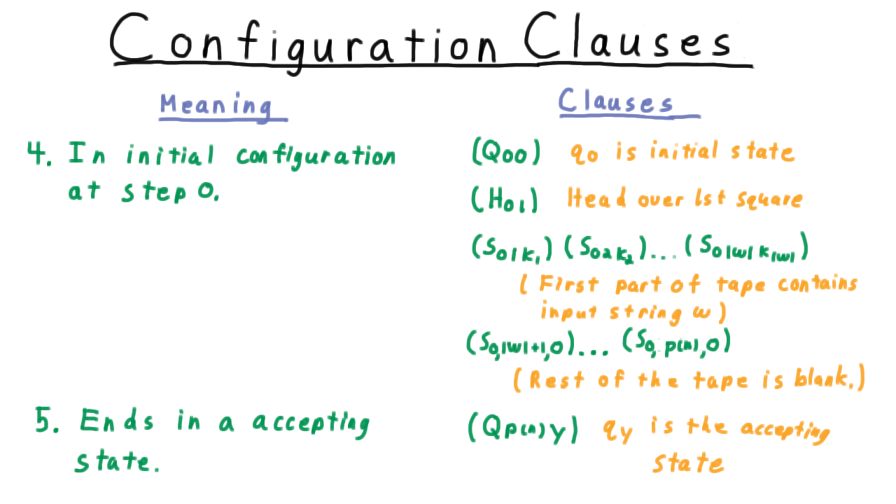
The machine must be in the initial configuration at step 0. This means that the initial state must be \(q_0.\)
The head must also be over the first position on the tape.
The first part of the tape contain the input \(w.\) Letting \(k_1 k_2\ldots k_{|w|}\) be the encoding for the input string, we
The rest of the tape must be blank to start.
These additional clauses are summarized here
Transition Clauses - (Udacity, Youtube)
Any assignment that truth assignment that satisfies these clauses we have defined so far indicated how the tableau should be filled out. Moreover, the tableau will always start out in the initial configuration and end up in an accepting one. What is not guaranteed yet it that the transitions between the configurations are valid.
To see how we can add constraints that will give us this guarantee, we’ll use this example.
Suppose that the transition functions tells us that if the machine is in state \(q_3\) and it reads a 1. Then it do one of two things:
- it can stay in \(q_0,\) leave the 1 alone, and move the head to the right,
- it can move to state \(q_4,\) write a 0 and move the head to the left.
To translate this rule into clauses for our formula, it’s useful to make a few definitions. First we need to enumerate the tape alphabet so that we can refer to the symbols by number.
Next, we define a tuple \((k,\ell,k',\ell',\delta)\) to be valid if the triple of the state \(q\_\{k'\}\), the symbol \(s\_\{\ell'\}\), and the direction delta is in the set delta of state \(q_k,\)
For example, the tuple \((3,2,0,2,R)\) is valid.
The first two numbers here indicate which transition rule applies (use the enumeration of the alphabet to translate the symbols), and the last three indicate what transition is being made. In this case, it is in the in the set defined by delta, so this is a valid transition.
On the other hand, the transition \((3,0,4,2,R)\) is invalid. The machine can’t switch to state 4, write a 1, and move the head to the right. That’s not one of the valid transitions given that the machine is in state 3 and that it just read a blank.
Now, there are multiple ways to create the clauses needed to ensure that only valid transitions are followed. Many proofs of Cook’s theorem start by writing out boolean expressions that directly express the requirement one of the valid transitions be followed. The difficulty with this approach is that the intuitive expression isn’t in conjunctive normal form and some boolean algebra is need to convert it. That is to say we don’t immediately get an intuitive set of short clauses to add to our formula. On the other hand, if we rule out in invalid transitions instead, then we do get a set of short intuitive clauses that we can just add to the formula.
To illustrate, in order to make sure that this invalid transition is never followed, for every step i and position j, we add a clause that starts like this.
\[ (\overline{ H_{ij}} \vee \overline{Q_{i3}} \vee \overline{S_{ij0}} \]
It starts with three literals that ensure the transition rules for being \(q_3\) and reading the blank symbol actually do apply. If the head isn’t in the position we’re talking about, the state isn’t q_3 , or the symbol being read isn’t the blank symbol, then the clause is immediately satisfied. The clause can also be satisfied if the machine behaves in any way that is different from what this particular invalid transition would cause to happen.
\[ \overline{ H_{(i+1)(j+1)}} \vee \overline{ Q_{(i+1)4}} \vee \overline{S_{(i+1)(j+1)2}} ) \]
The head could move differently, the state could change differently, or a different symbol could be written.
Another way to parse this clause is as saying if the \((q_3, \sqcup)\) transition rule applies, then the machine can’t have changed in this particular invalid way. Logically, remember that A implies not B is equivalent to not A or not B. That’s the logic we are using here.
Transition Clauses Cont - (Udacity, Youtube)
Now let’s state the general rule for creating all the transition clauses. Recall that a tuple \((k,\ell,k',\ell',\Delta)\) is valid if switching to state \(q\_\{k'\}\), writing out symbol \(\ell'\) and moving in direction \(\Delta\) is an option given that the machine is currently in state \(q_k\) and reading symbol \(s\_\ell.\)
For every step \(i,\) position \(j,\) and invalid tuple then, we include in the formula this clause. The first part tests to whether the truth assignment is such that the transition rule applies
and the next three ensure that this invalid transition wasn’t followed. This is just the generalization of the example we saw earlier.
Cook Levin Summary - (Udacity, Youtube)
We’re almost done with the proof that satisfiability is NP-complete, but before making the final arguments I want to remind you of what we’re trying to do.
Consider some language in NP, and suppose that someone wants to be able to determine whether strings are in this language. The Cook-Levin theorem argues that because L is in NP, there is a nondeterministic Turing machine that decides it, and it uses this fact to create a function computable in polynomial time that takes any input string x and outputs a boolean formula that is satisfiable if and only if the string x is in L.
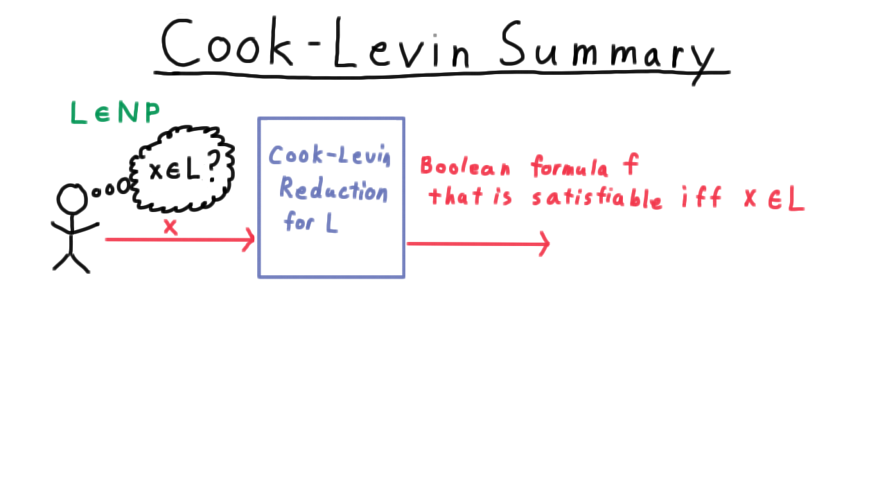
That way, any algorithm for deciding satisfiability in polynomial time would be able to decide every language in NP.
Only two questions remain.
- “Is the reduction correct?”
- “Is it polynomial in the size of the input?”
Let’s consider correctness first. If \(x\) is in the language, then clearly the output formula \(f\) is satisfiable. We can just use the truth assignment that corresponds to an accepting computation of the nondeterministic Turing machine that accepts \(x.\) That will satisfy the formula \(f.\) That much is certainly true.
How about the other direction? Does the formula being satisfiable imply that x is in the language? Take some satisfying assignment for \(f.\) As we’ve argued,
- the corresponding tableau is well-defined. Only one of the state variables can be true at any time step, etc,
- the tableau starts in the initial configuration,
- every transition is valid,
- the configuration sequence ends in an accepting configuration.
That’s all that is needed for a nondeterministic Turing machine to accept, so this direction is true as well.
Now, we have to argue that the reduction is polynomial.
First, I claim that the running time is polynomial in the output formula length. There just isn’t much calculation to be done besides iterating over the combination of steps, head positions, states, and tape symbols and printing out the associated terms of the formula.
Second, I claim that the output formula is polynomial in the input length. Let’s go back and count

These clauses pertaining to the states require order \(p(n) \log n\) string length. The number of states of the machine is a constant in this context. The \(p\) factor comes from the number of steps of the machine. The \(\log n\) factor comes from the fact that we have to distinguish the literals from one another. This requires log n bits. In all these calculations, that’s where the log factor comes from.
For the head position, we have \(O(p(n)3 log n)\) string length one factor of p from the number of time steps and two from all pairs of head positions.
There are \(O(p^2)\) combinations of steps and squares, so this family of clauses requires \(O(p^2 log n)\) length as well.

The other clauses related to individual configurations come from the start and end states. The initial configuration clause is a mere \(O(p(n) \log n)\)
The constraint that the computation be accepting only requires \(O(\log n)\) string length.
The transition clauses might seem like they would require a high order polynomial of symbols, but remember that the size of the nondeterministic Turing machine is a constant in this context. Therefore, the fact that we might have to write out clauses for all pairs of states and tape symbols doesn’t affect the asymptotic analysis. Only the range of the indices i and j depend on the size of the input string, so we end up with \(O(p^2 \log n).\)
Adding all those together still leaves us with a polynomial string length. So, yes, the reduction is polynomial! And Cook’s theorem is proved.
Conclusion - (Udacity, Youtube)
Congratulations!! You have seen that one problem, satisfiability, captures all the complexity of P versus NP problem. An efficient algorithm for Satisfiability would imply P = NP. If P is different than NP then there can’t be any efficient algorithm for satisfiability. Satisfiability has efficient algorithms if and only if P = NP.
Steve Cook, a professor at the University of Toronto, presented his theorem on May 4, 1971 at the Symposium on the Theory of Computing at the then Stouffer’s Inn in Shaker Heights, Ohio. But his paper didn’t have an immediate impact as the Satisfiability problem was mainly of interest to logicians. Luckily a Berkeley professor Richard Karp also took interest and realized he could use Satisfiability as a starting point. If you can reduce Satisfiability to another NP-complete problem than that problem must be NP-complete as well. Karp did exactly that and a year later he published his famous paper on “Reducibility among combinatorial problems” showing that 21 well-known combinatorial search problems that were also NP-complete, including, for example, the clique problem.
Today tens of thousands of problems have been shown to be NP-complete, though ones that come up most often in practice tend to be closely related to one of Karp’s originals.
In the next lesson, we’ll examine some of the reductions that prove these classic problems to be NP-complete, and try to convey a general sense for how to go about finding such reductions. This sort of argument might come in handy if you need to convince someone that a problem isn’t as easy to solve as they might think.