Computability, Complexity, and Algorithms
Charles Brubaker and Lance Fortnow
Computability, Complexity, and Algorithms
Charles Brubaker and Lance Fortnow
Dynamic Programming - (Udacity)
Intro to Algorithms - (Udacity, Youtube)
In this and the remaining lessons for the course, we turn our attention to the study of polynomial algorithms. First, however, a little perspective.
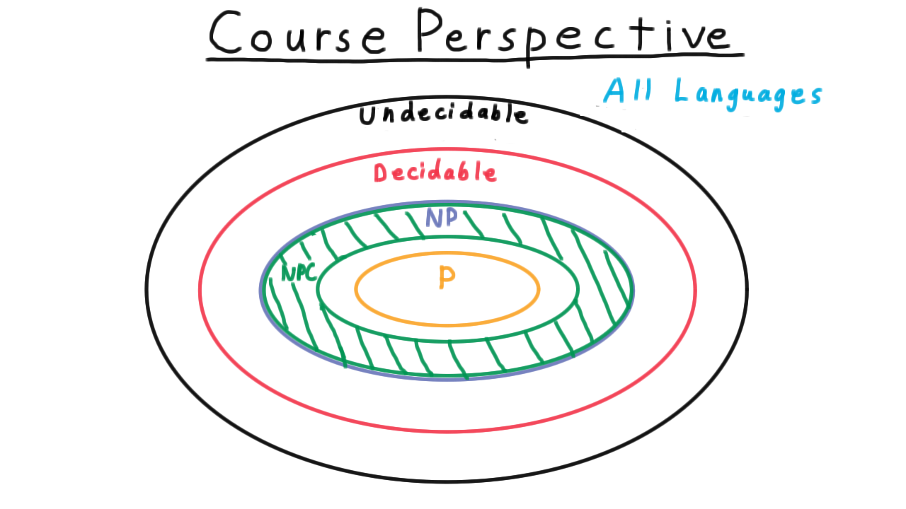
In the beginning of the course, we defined the general notion of a language. Then we began to distinguish between decidable languages and undecidable ones. Remember that there were uncountably many undecidable ones but only countable decidable ones. In comparison, the decidable ones should be infinitesimally small, but we’ll give the decidable ones this big circle anyway because they are so interesting to us.
In the section of the course on Complexity, we considered several subclasses of the decidable languages:
- P which consisted of those languages decidable in polynomial time time,
- NP, which consisted of the languages that could be verified in polynomial time (represented with the purple ellipse here, and that includes P.),
- and then we distinguished certain problems in NP which were the hardest and we called these NP-complete. We visualize these in this green band at the outside of NP, since if any one of these were in P, then P would expand and swallow all of NP (or equivalently, NP would collapse to P).
In this section, we are going to focus on the class P, the set of polynomially decidable languages. The overall tone here will feel a little more optimistic. In the previous sections of the course, many of our results were of a negative nature: “No, you can’t decide that language,” or “No, that problem isn’t tractable unless P=NP.” Here, the results will be entirely positive. No longer will we be excluding problems from a good class; we will just be showing that problems are in the good class P: “Yes, you can do that in polynomial time”, or “it’s even a low order polynomial and we can solve huge instances in practice.”
It certainly would be sad if this class P didn’t contain anything interesting. One rather boring language in P, for instance, is the language of lists of numbers no greater than 5. Thankfully, however, P contains some much more interesting languages, and we use the associated algorithms everyday to do things like sort email, find a route to a new restaurant, or apply filters to enhance the photographs we take. The study of these algorithms is very rich, often elegant, and ever changing, as computer scientists all over the world are constantly finding new strategies and expanding the set of languages that we know to be in P. There are non-polynomial algorithms too, but since computer scientists are most concerned with practical solutions that scale, they tend to focus on polynomial ones, as will we.
In contrast to the study of computability and complexity, the study of algorithms is not confined to a few unifying themes and does not admit a clear overall structure. Of course, there is some structure in the sense that many various real-world applications can be viewed as variations on the same abstract problem of the type we will consider here. And, there are general patterns of thinking, or design techniques, that are often useful. We will discuss a few of these. And sometimes even abstract problems are intimately related, when on the surface the may not seem similar. We will see this happen too. Yes, despite these connections, in large part, problems tend to demand that they be solved by their own algorithm that involves a particular ingenuity, at least if they are to yield up the best running time.
If the topic is so varied, how then can a student understand algorithms in any general way, or become better at finding algorithms for his own problems? There are two good, complementary ways.
- First, and most important, is practice. The more problems that you try to solve efficiently, the better you will become at it and the more perspective you will gain.
- Second, is to study the classic and most elegant algorithms in detail. Here, we will do this for a few problems often not covered in undergraduate courses.
Even better is if you can combine the two approaches. Don’t just follow along with pen and paper. Pause and see if you can anticipate the next step and work ahead both on the algorithm and the analysis. Keep that advice in mind throughout our discussion of algorithms.
Introduction - (Udacity, Youtube)
Our first lesson is not on one algorithm in particular but on a design technique called dynamic programming. This belongs in the same mental category as divide and conquer: it’s not a algorithm in itself because it doesn’t provide fixed steps to follow; rather, it’s a general strategy for thinking about problems that often produces an efficient algorithm.
The term dynamic programming, by the way, is not very descriptive. The word programming is used in an older sense of the word that refers to any tabular method, and the word dynamic was used just to make the technique sound exciting.
With those apologies for the name, let’s dive into the content.
Optimal Similar Substructure - (Udacity, Youtube)
The absolutely indispensable element of dynamic programming is what we’ll call an optimal similar substructure (often simply called optimal substructure). By this, I mean that we have some hard problem that we want to solve, and we think to ourselves, “oh, if only had the answer to these two similar, smaller subproblems this would be easy.” Because the subproblems are similar to the original, we can keep playing this game, letting the problems get smaller and smaller until we’ve reached a trivial case.
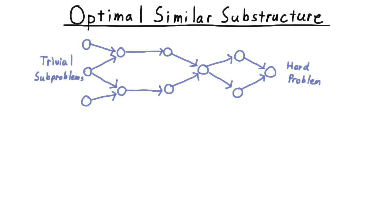
Well at first, this feels like an ideal case for recursion. Since the subproblems are similar, perhaps we can use the same code and just change the parameters. Starting from the hard problem on the right, we could recurse back to the left. The difficulty is that many of the recursive paths visit the same nodes, meaning that such a strategy would involve wasteful recomputaion.
This is sometimes called one of the perils of recursion, and it’s often illustrated to beginning programmers with the example of computing the Fibonacci sequence. Each number in the Fibonacci sequence is the sum of the previous two with the first two numbers both being 1 to get us started. That is,
This hard problem of computing the \(n\)th number in the sequence depends on solving the slightly easier problems of computing the \((n-1)\)th and the \((n-2)\)th elements in the sequence.
Computing the \((n-1)\)th element depends on knowing the answer for \(n-2\) and \(n-3\). Computing the \((n-2)\)th depends on know the answer for \(n-3\) and \(n-4\) and so forth.
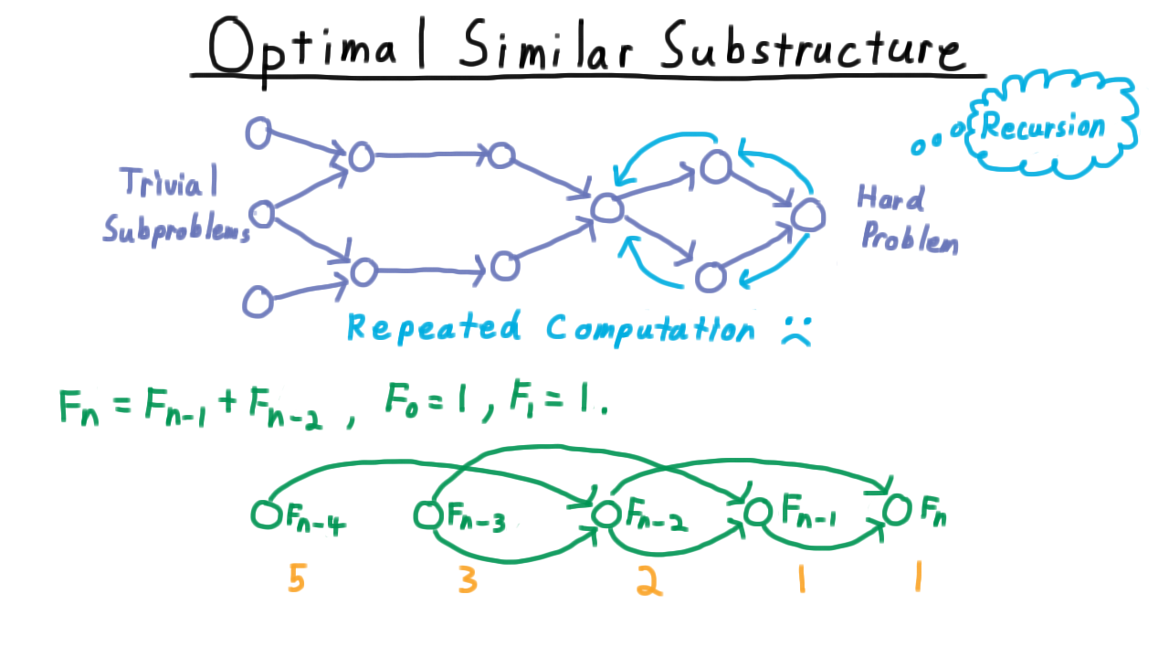
Thinking about how the recursion will operate, notice that we’ll need to compute \(F_{n-2}\) once for \(F_n\) and once for \(F_{n-1},\) so there’s going to be some repeated computation here, and its going to get worse the further to the left we go.
How bad does it get? The top level problem of computing the \(n\)th number will only be called once and he will find the problem of computing the \((n-1)\)th number once.
Computing \(n-2\) needs to happen once for each time that the two computations that depend on it are called: once for \(n-1\) and once for \(n.\)
Similarly, computing \(n-3\) needs to happen once for every time that problems that depend on it are called, so it gets called two plus one for a total of three time.
Notice that each number here is the sum of the two numbers to the right, so this is the Fibonacci sequence, and the number of times that the \((n-k)\)th number is computed will be equal to the \(k\)th Fibonacci number, which is roughly the golden ratio raised to the \(k\)th power, \( \frac{\varphi^k}{\sqrt{5}}.\) The recursive strategy is exponential!
There are two ways to cope with this problem of repeated computation.
- One is to memoize the answers to the subproblems. After we solve it the first time, we write ourselves a memo with the answer, and before we actually do the work of solving a subproblem we always check our wall of memos to see if we have the answer already.
- Alternatively, we can solve the subproblems in the right order, so that anytime we want to solve one of the problems we are sure that we have solved its subproblems already.
The latter can always be done, because the dependency relationships among the subproblems must form a directed acyclic graph. If there were a cycle, then we would have circular dependencies and recursion wouldn’t work either. We just find an appropriate ordering of the subproblems, so that all the edges go from left to right and then we solve the subproblems in the left to right order. This is the approach we’ll take for this lesson. It tends to expose more of the underlying nature of the problem and to create faster implementations than using recursion and memoizing.
Edit Distance Problem - (Udacity, Youtube)
The first problem we’ll consider is the problem of sequence alignment or edit distance. This often comes up in genetics or as part of spell-checkers.
For example, suppose that we are given two genetic sequences and we want to line them up as best as possible, minimizing the needed insertions, deletions and changes to the characters that would be needed to switch one to the other; and we’ll do this according to some cost function that represents how likely these changes are to have occurred in nature.
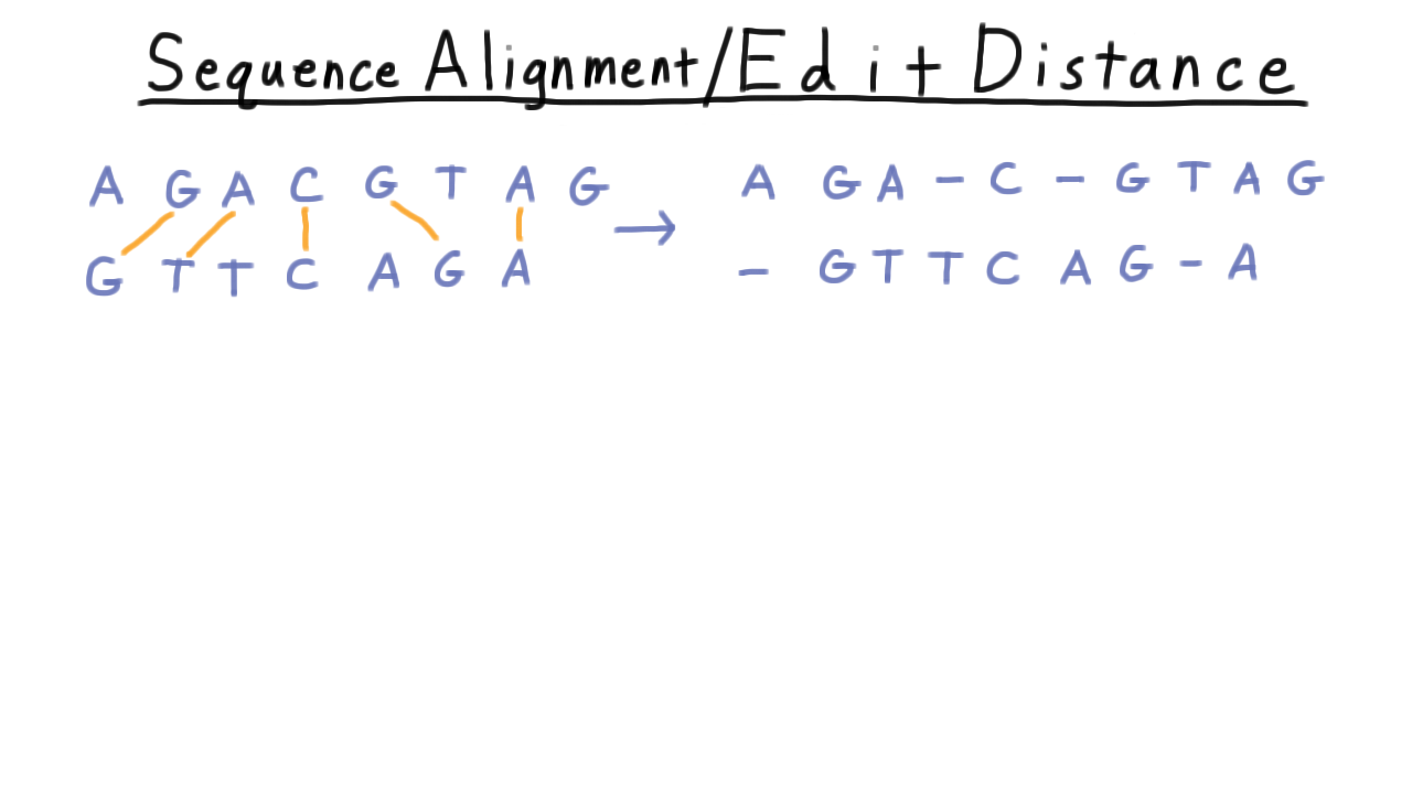
In general, we say that we are given two sequences \(X\) and \(Y\) over some alphabet and we want to find an alignment between them–that is a subset of the pairs between the sequences so that each each letter appears only in one pair and the pairs don’t cross, like in the example above.
For completeness, we give the formal definition of an alignment, though for our purposes the intuition given above is sufficient.
An alignment is a subset \( A \) of \(\{1,\ldots,n\} \times \{1,\ldots,m\}\) such that for any \((i,j),(i',j') \in A\),
\[ i \neq i'\;\;\; j \neq j, \;\;\; \mbox{and}\;\;\; i < i' \Longrightarrow j < j'.\]
The cost of an alignment comes from two sources:
- one is the number of unmatched characters, which we can write as \(n+m - 2|A|\). This corresponds to the number of insertions or deletions–or matching with the dash character in our figures.
- The other part of the cost comes from matching two of the characters.
Typically, this is zero when the two characters are the same.
In total
\[c(A) = n + m - 2|A| + \sum_{(i,j) \in A} \alpha(x_i,y_j). \]
The problem then is to find an alignment of the sequences that minimizes this cost.
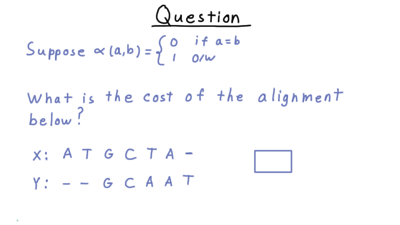
Sequence Alignment Cost - (Udacity)
To make sure we understand this cost function, I want you to suppose that the function alpha is zero if the two characters are the same and 1 otherwise, and to calculate the cost of the alignment given below.
Prefix Substructure - (Udacity, Youtube)
The key optimal substructure for the sequence alignment problem comes from aligning prefixes of the sequence that we want to align. We define \(c(i,j)\) to be the minimum cost of aligning the \(i\) characters of \(X\) with the first \(j\) characters of \(Y.\) Since \(X\) has \(m\) characters and \(Y\) has \(m,\) our overall goal is to compute \(c(m,n)\) and the alignment that achieves it.
Let’s consider problem of calculating \(c(m,n).\) There are three cases consider.
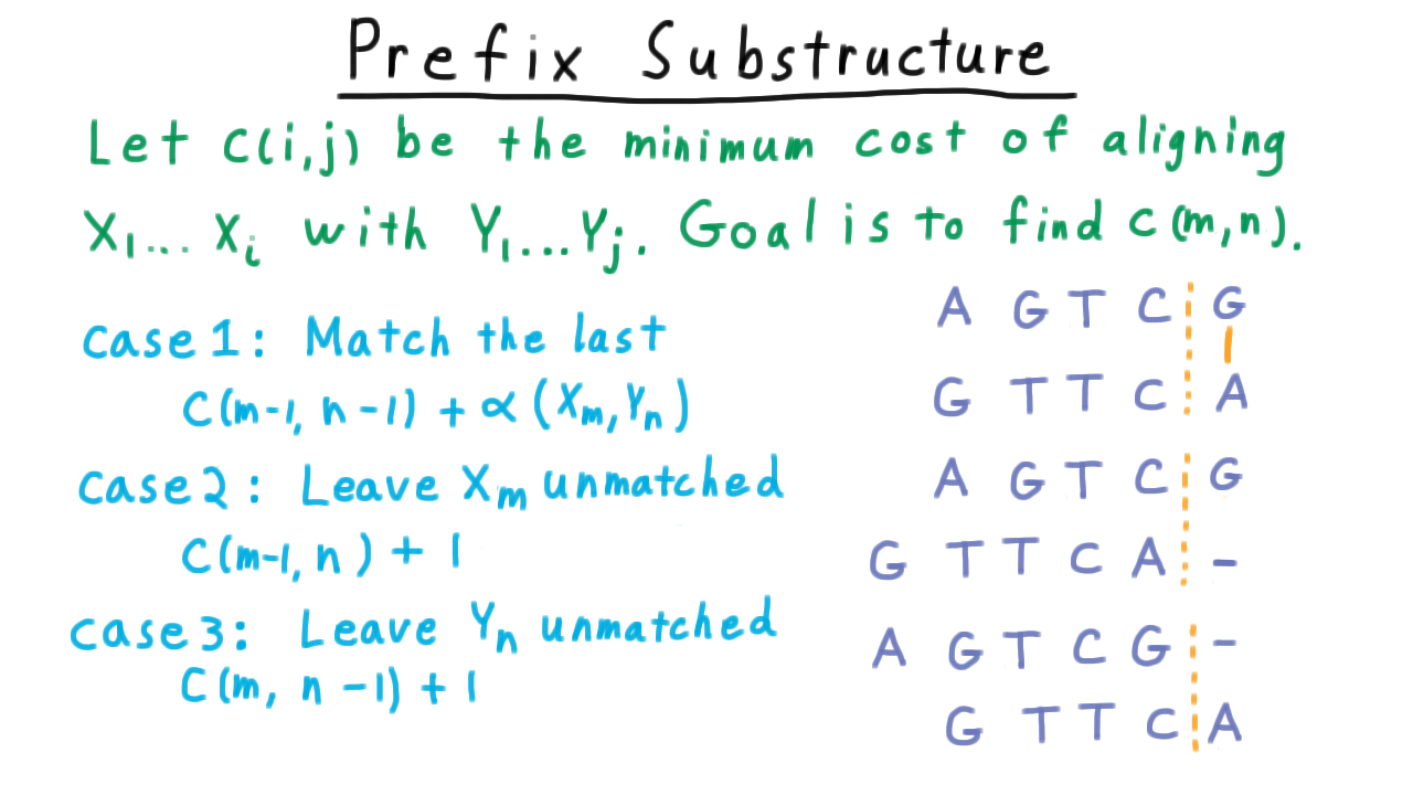
First, suppose that we match the last two characters of the sequences together. Then the cost would be the minimum cost of aligning the prefix from \(m-1\) of \(X\) and the prefix through \(n-1\) of \(Y,\) plus the cost associated with matching the last two characters together.
Another possibility is that we leave the last character of the \(X\) sequence unmatched. Then the cost would be the minimum cost of aligning the prefix from \(m-1\) of \(X\) and the prefix through \(n\) of \(Y,\) plus 1 for leaving \(X_m\) unmatched.
And the last case where we leave \(Y_n\) unmatched instead is analogous.
Of course, since \(c(m,n)\) is defined to be the minimum cost aligning the sequences, it must be the minimum of these three possibilities. Notice, however, that there was nothing special about the fact that we were using n and m here, and the same argument applies to all combination of i,j. The problems are similar. Thus, in general,
\[ c(i,j) = \min \{c(i-1,j-1) + \alpha(X_i,Y_j), c(i-1,j) + 1, c(i,j+1) + 1 \}. \]
Including the base cases where the cost of aligning a sequence with the empty sequence is just the length of the sequence,
\[ c(0,j) = j \;\;\; \mbox{and}\;\;\; c(i,0) = i \]
we have a recursive formulation–the optimal solution expressed in terms of optimal solutions to similar subproblems.
Sequence Alignment Algorithm - (Udacity, Youtube)
As you might imagine, a straightforward recursive implementation would involve an unfortunate amount of recomputation, so we’ll look for a better solution. Notice that it is natural to organize our subproblems in a grid like this one.
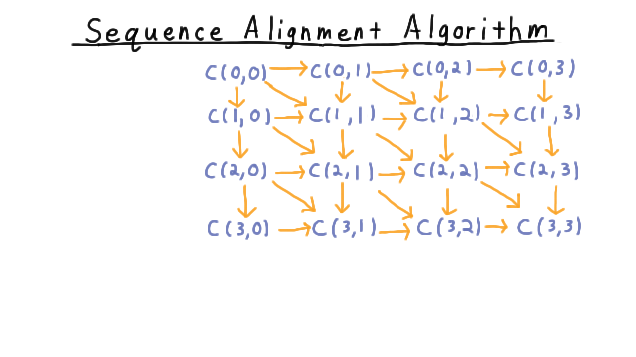
Knowing C(3,3) the cost of aligning the full sequence depends on knowing C(3,2) C(2,2) and C(2,3).
Knowing C(2,3) depends on knowing C(2,2), C(1,2), and C(1,3), and indeed in general, to figure out any cost, we need to know the cost north, west and northwest in this grid.
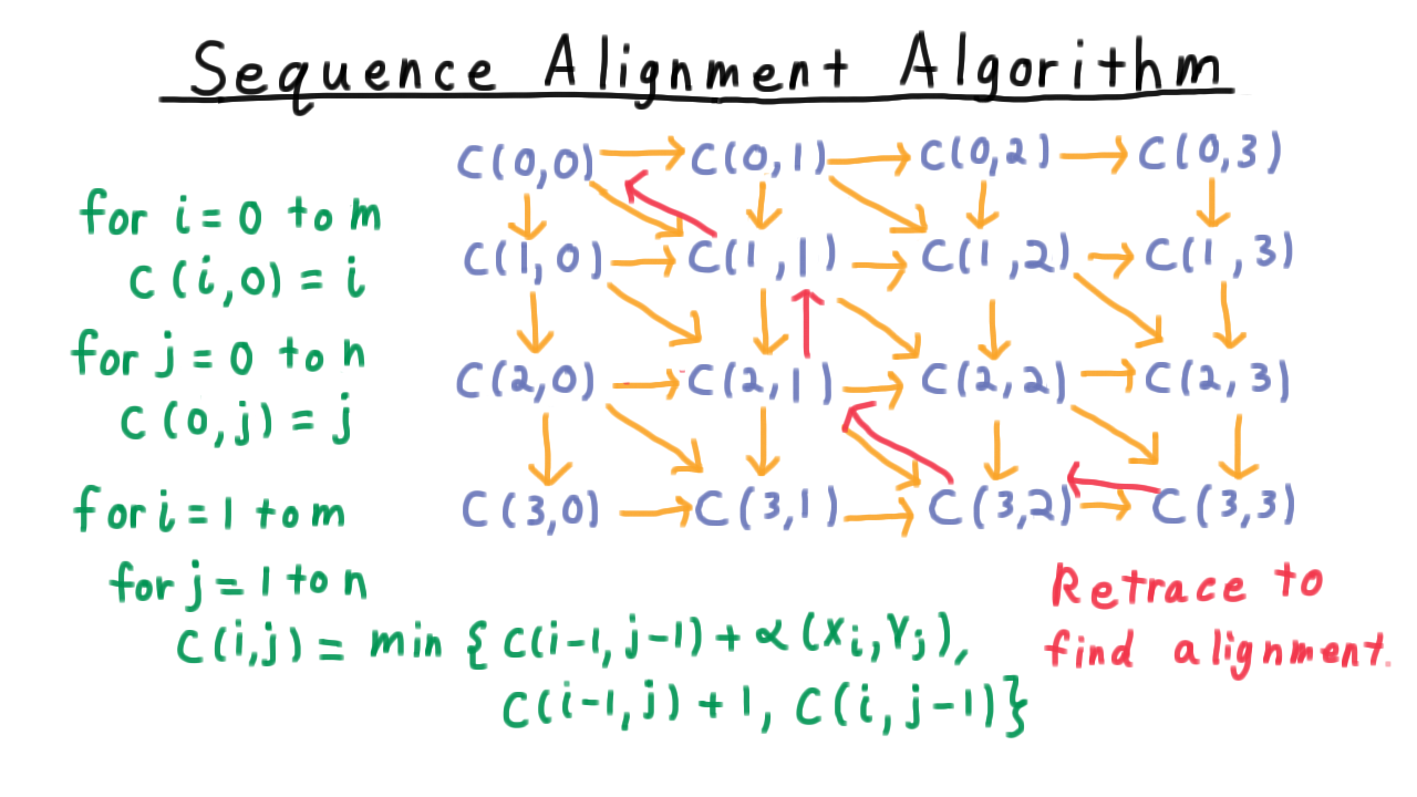
These dependencies form a directed acyclic graph, and we can linearize them in a number of ways. We might in scanline order, left to right, or even along the diagonals. We’ll keep it simple and do a scanline order. First, We need to fill in the answers for the base cases, and then, it’s just a matter of passing over the grid and taking the minimum of the three possibilities outlined earlier. Once we’ve finished, we can retrace our steps by looking at west, north, and northwest neighbors and figuring out what step we took, and that will allow us to reconstruct the alignment.
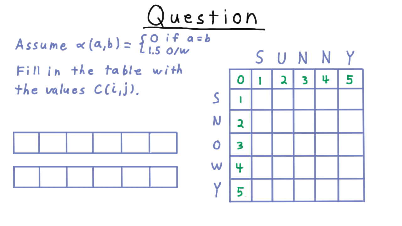
Sequence Alignment Exercise - (Udacity)
Let’s practice computing these costs and extracting the alignment with an exercise. We’ll align snowy with sunny and we’ll use an alpha value with a penalty of 1.5 for flipping an character. This makes flipping a character more expensive than an insertion or deletion.
Compute the minimum cost and write out a minimum cost alignment here, using the single dash to indicate where a character isn’t matched.
Sequence Alignment Summary - (Udacity, Youtube)
To sum up the application of dynamic programming to the sequence alignment problem, recall that we gave an algorithm, which given two sequences of lengths m and n found a minimum cost alignment in \(O(mn)\) time. We did a constant amount of work for each element in the grid.
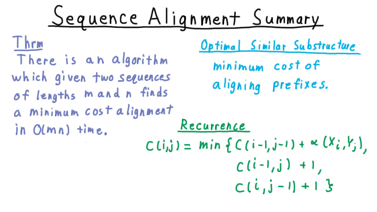
Dynamic programming always relies on the existence of some optimal similar substructure. In this case, it was the minimum of cost aligning prefixes of the sequences that we wanted to align. The key recurrence being that the cost of aligning the first i characters of one sequence with the first j other other was the minimum of the costs of matching the last characters, leaving the last character of the first sequence unmatched, or the cost of leaving the last character of the second sequence unmatched.
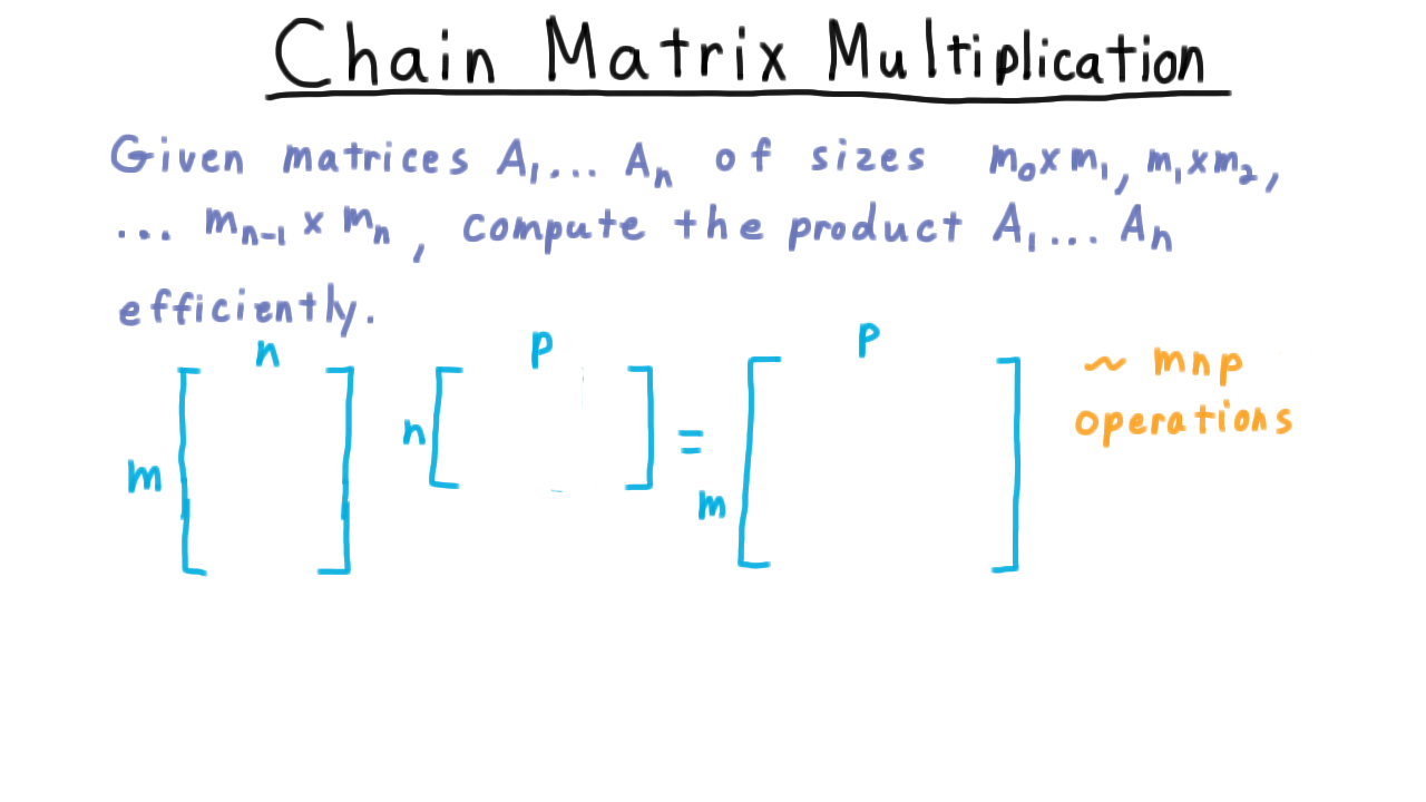
Chain Matrix Multiplication - (Udacity, Youtube)
Now we turn to another problem that we’ll be able to tackle with the dynamic programming paradigm, Chain Matrix Multiplication. We are given a sequence of matrices of sizes \(m_0 \times m_1,\) \(m_1 \times m_2,\) etc, and we want to compute their product efficiently. Note, how dimensions here are arranged so that such a product is always defined. The number of columns in one matrix always matches the number of rows in the next.
First, recall that the product of an \(m \times n\) matrix with an \(n \times p\) matrix produces an \(m \times p\) matrix and that the cost of computing each entry is \(n.\) Each entry can be thought of as the vector dot product between the corresponding row of the first matrix and the column of the second. Both vectors have \(n\) entries. In total, we have about \(mnp\) additions and as many multiplications.
Next, recall that matrix multiplication is associative. Thus, as far as the answer goes it doesn’t matter whether we multiply \(A\) and \(B\) first and then multiply that product by \(C,\) or if we multiply \(B\) and \(C\) first and then multiply that product by \(A.\)
\[(AB)C = A(CB)\]
The product will be the same, but the number of operations may not be.
Let’s see this with an example. Consider the product of an \(50 \times 20\) matrix \(A\) with a \(20 \times 50\) matrix B with a \(50 \times 1\) matrix \(C.\), and let’s count the number of multiplications using both strategies.
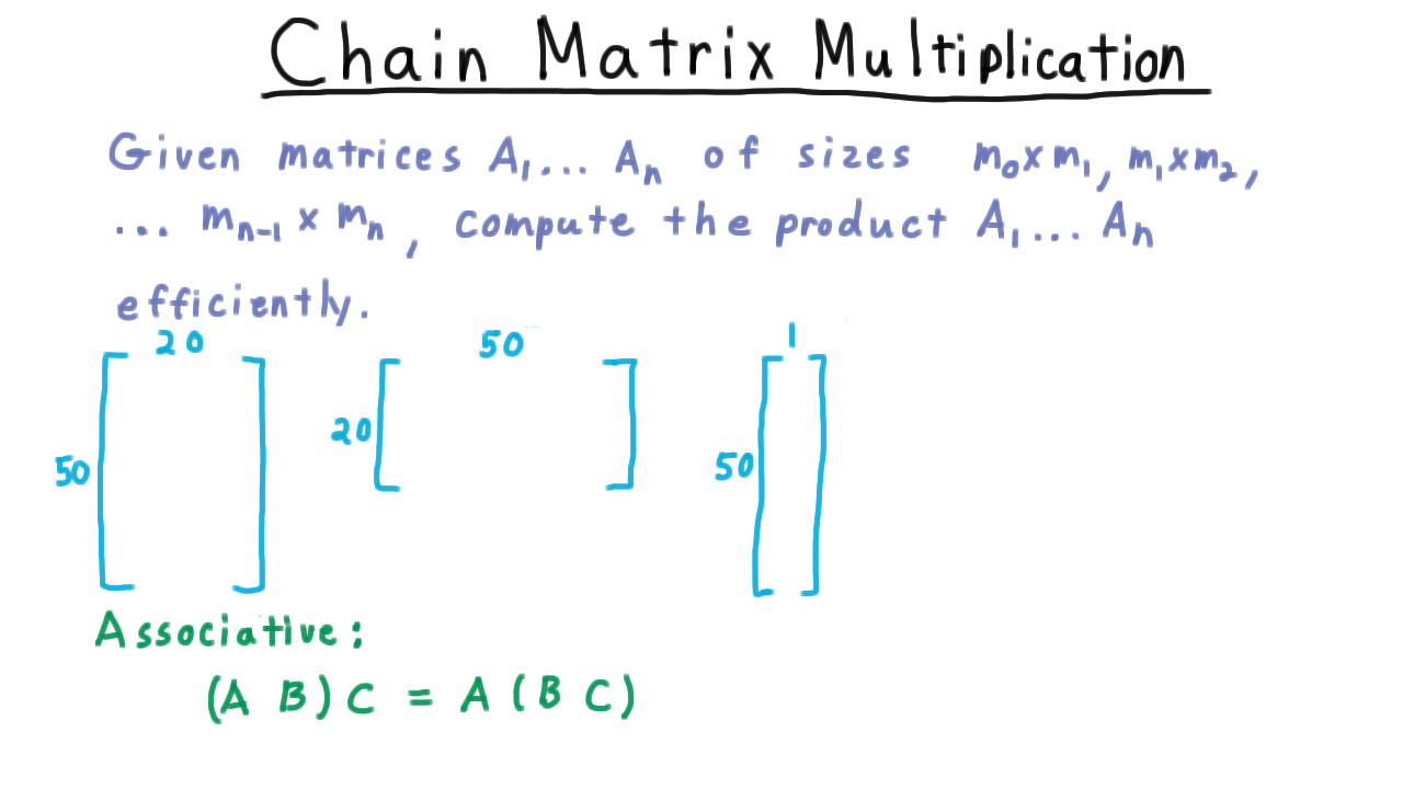
If we multiply A and B first, then we spend \(50 \cdot 20 \cdot 50\) on computing \(AB.\) This matrix will have 50 rows and 50 columns, so its product with \(C\) will take \(50 \cdot 50 \cdot 1\) multiplications for a total of
\[ 50 \cdot 20 \cdot 50 + 50 \cdot 50 \cdot 1= 52,500. \]
On the other hand, if we multiply B and C first, this costs \(20 \cdot 50 \cdot 1.\) This produces a \(20 \times 1 \) and multiplying it by \(A\) costs \(50 \cdot 20 \cdot 1\) for total of only
\[ 20 \cdot 50 \cdot 1 + 50 \cdot 20 \cdot 1 = 2000\]
a big improvement. So, it’s important to be clever about the order we choose for multiplying these matrices.
Subchain Substructure - (Udacity, Youtube)
In dynamic programming, we always look for optimal substructure and try to find a recursive solution first.
We can gain some insight into the substructure by writing out the expression trees for various ways of placing parentheses. Consider these examples.
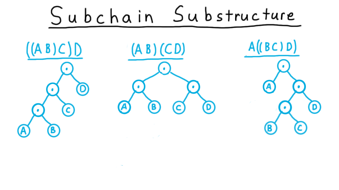
This suggests that we try all possible binary trees and pick the one that has the smallest computational cost.
Starting from the top level, we would consider all \(n-1\) ways of partitioning into left and right subtrees, and for each one of these possible partitions, we would figure out the cost of computing the subtrees and then multiplying them together.
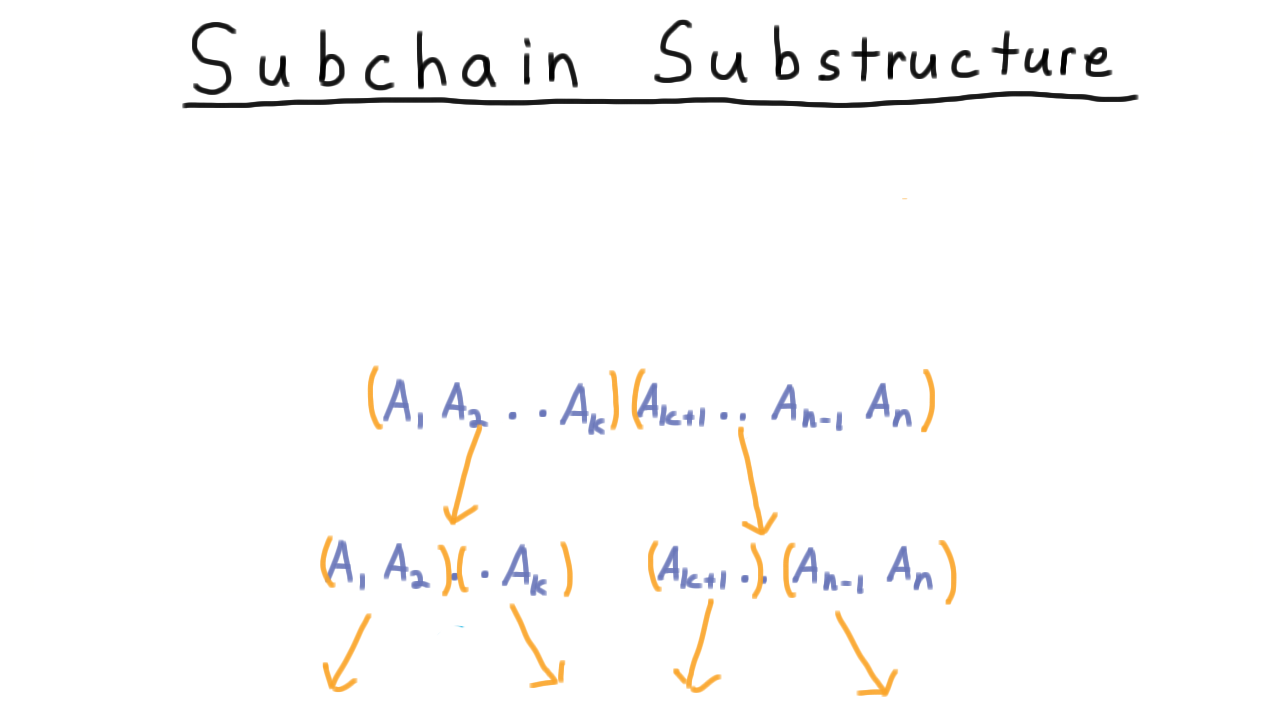
To figure out the cost of the subtrees themselves, we would need to consider all possible partitions into left and right subtree and so forth.
More precisely, let \(C(i,j)\) be the minimum cost of multiplying \(A_i\) through \(A_j.\) For each way of partitioning this range, the cost is the minimum cost of computing each subtree, plus the cost of combining them, and we just want to take the minimum over all such partitions.
\[C(i,j) = \min_{k: i \leq k < j} C(i,k) + C(k+1,j) + m_{i-1}m_k m_j\]
The base case is the product of just one matrix, which doesn’t cost anything.
\[C(i,i) = 0.\]
CMM Algorithm - (Udacity, Youtube)
Now that we have this recursive formulation, we are ready to develop the algorithm. Let’s convince ourselves first that the recursive formulation would indeed involved some needless recomputation.
Take the two top-level partitions of \(ABCDE\), on the one hand \((ABC)\) and \((DE)\) and on the other \((ABCD)\) and \(E\) .
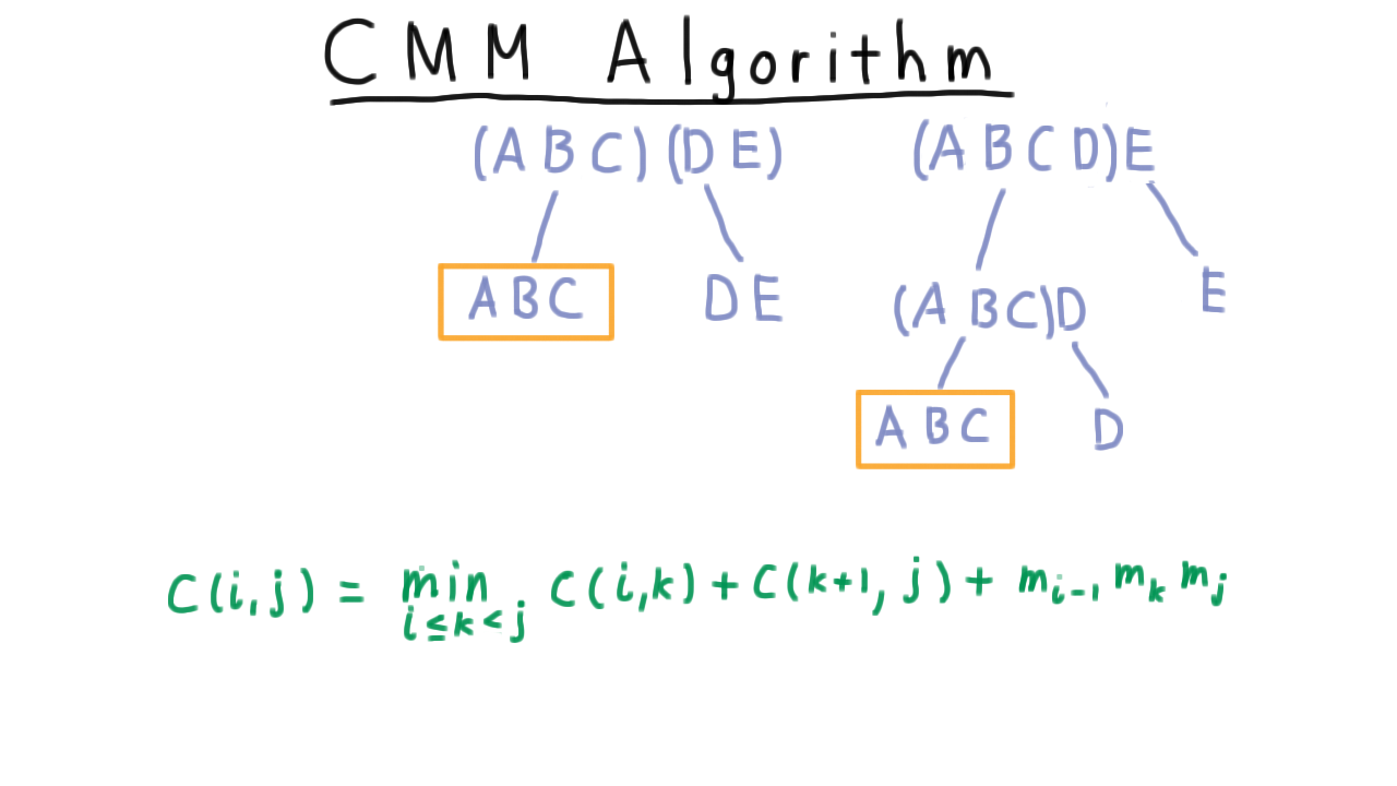
Clearly, we will have to compute the minimum cost of multiply \((ABC)\) in the left problem. But we are going to have to compute it on the right as well, since we need to consider pulling \(D\) off from the \((ABCD)\)chain as well. We end up re-doing all of the work involved in figuring out how to best multiply ABC over again. As we go deeper in the tree, things get recomputed more and more times.
Fortunately for us, there are only n choose two subproblems, so we can create a table and do the subproblems in the right order.
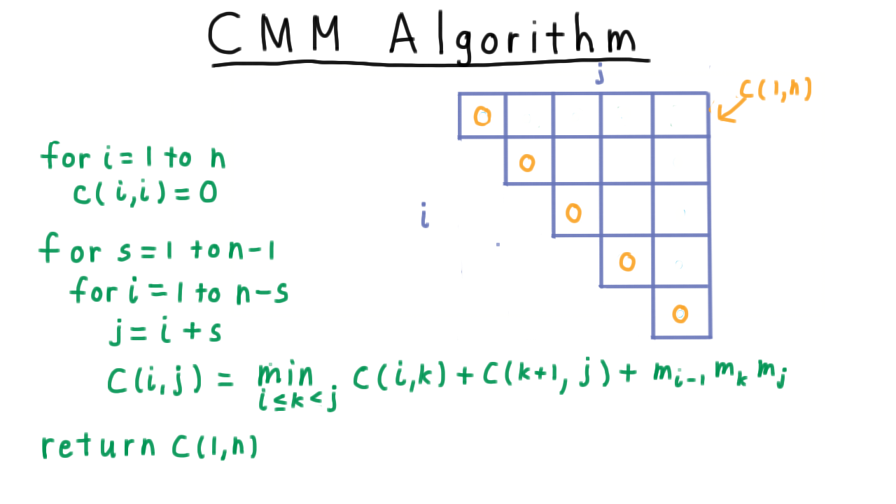
The entries along the diagonal are base cases which have cost zero. A product of one matrix doesn’t case anything. Our goal is to compute the value in the upper right corner \(C(1,n).\)
Consider which subproblems this depends on. When the split reprsented by \(k\) is \(k=1\), we are considering these costs \(C(1,1)\) and \(C(2,n).\) When \(k=2,\) we consider the problems \(C(1,2)\) and \(C(3,n)\). In general, every entry depends on all the elements the left and down in the table.
There are many ways to linearize this directed acyclic graph of dependence, but the most elegant is to fill in the diagonals going towards the upper right corner. In the code, we have let s indicate which diagonal we are working on. The last step, of course, is just to return this final cost.
The binary tree that produced this cost can be reconstructed from the k that yielded these minimum values. We just need to remember the split we used for each entry in the table.
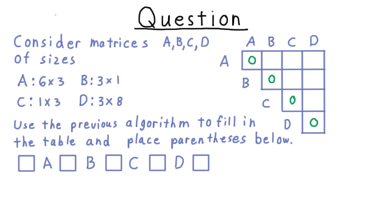
CMM Exercise - (Udacity)
Let’s do an exercise to practice this chain matrix multiplication algorithm. Consider matrices ABCD with dimensions given below. Use the dynamic programming algorithm to fill out the table to the right, and then place the parentheses in the proper place below to minimize the number of scalar multiplications. Don’t use more parentheses than necessary in your answer.
CMM Summary - (Udacity, Youtube)
Let’s summarize what we’ve learned about the Chain Matrix Multiplication problem. There is algorithm which given the dimension of the n matrices finds an expression tree that computes the product with the minimum number of multiplications in \(O(n^3)\) time. Recall that there were order \(n^2\) entries in the table and we spent order \(n\) time figuring out what value to write in each one.
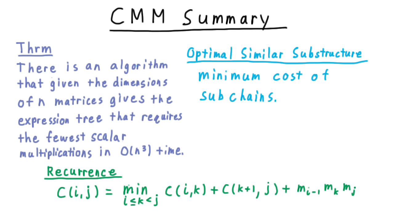
The optimal similar substructure that we exploited was the minimum cost of evaluating the subchains the key recurrence saying that the cost of each partition is the cost of evaluting each part plus the cost of combining them, and of course, we want to take the minimum cost over all such partitions.
All Pairs Shortest Path - (Udacity, Youtube)
Now, we turn to out last example of dynamic programming and consider the problem of finding shortest paths between all pairs of vertices in a graph.
If you are rusty on ideas like paths in graphs and Dijkstra’s algorithm, it might help to review these ideas before proceeding with this part of the lesson.
Note that the idea of shortest is in terms weights or costs on the edges. These might be negative, so we don’t refer to them as lengths or distances themselves to avoid confusion, but we retain the word shortest with regard to the path instead of saying “lightest” or “cheapest.” Unfortunately, the use of this mixed metaphor is standard.
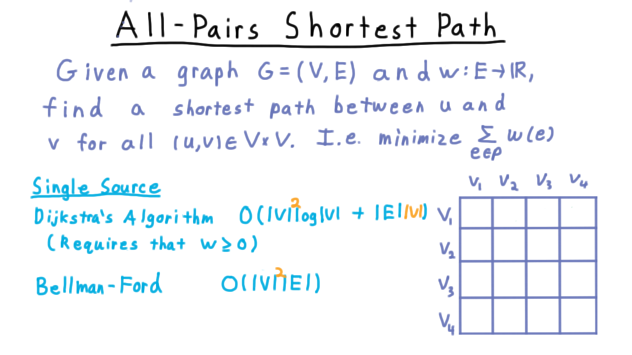
Here is the formal statement of the problem. Given a graph, and a function over the edges assigning them weights, we want to find the shortest (i.e. the minimum weight) path between every pair of vertices.
Recall that for the single source problem, where we want to figure out the shortest path from one vertex to all others, we can use Dijkstra’s Algorithm, which takes \(O(V log V + E)\) time, when used with a Fibonacci queue. But this algorithm requires that the weights all be non-negative, an assumption that we don’t want to make.
For graphs with negative weights, the standard single source solution is the Bellman-Ford algorithm, which takes time \(O(VE)\).
Now we can run these algorithms multiple times, once with each vertex as the source. If we visualize the problem of finding the shortest path between all pairs as filling out this table. Each run of Dijkstra or Bellman-Ford would fill out one row of the table.
We are running the algorithm V times, so we just add a factor of V to the running times.
For the case where we have negative weights on the edges and the graph is dense, we are looking at a time that is V to the fourth power here. Using dynamic programming, we’re going to be able to do better.
Shortest Path Substructure - (Udacity, Youtube)
Since we are using dynamic programming, the first thing we look for is some optimal similar substructure. Recall that the key realization in understanding the single source shortest path algorithms like Dijkstra and Bellman-Ford was that subpaths of shortest paths are shortest paths. So if this shortest path between u and v happens to go through these two vertices x and y, then this subpath between x and y must be a shortest path. If there were a shorter one, then it could replace the subpath in the path from u to v to produce a shorter u-v path. This type of argument is sometimes called cut and paste for obvious reasons.
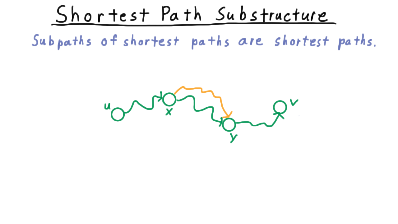
By the way, throughout I’ll use the squiggly lines to indicate a path between two vertices and a straight line to indicate a single edge.
Unfortunately, by itself this substructure is not enough.
Sure, we might argue that a shortest path from u to v take a shortest path from u to a neighbor of v first, but how do we find those shortest paths. The subproblems end up having circular dependencies.
One idea is include the notion of path length defined by the number of edges used. If we knew all shortest paths that only used \(k-1\) edges, then by examining the neighbors of v, we could figure out a shortest paths with k edges to v. We’ll let \(\delta(u,v,k)\) be the weight of the shortest path that uses at most \(k\) edges. Then the recurrence is that \(\delta(u,v,k)\) is the minimum of
- \(\delta(u,v,k-1)\)–this is where we don’t use that potential \(k\)th edge
- the minimum of the distances from \(u\) to the neighbors of \(v\) using only \(k-1\) edges, plus the weight of that last step.
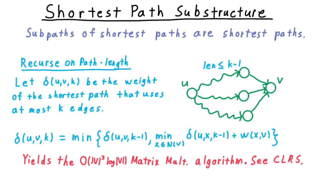
This strategy works, and it yields the matrix multiplication shortest paths algorithm that runs in time \(O(V^3 log V).\) See CLRS for details.
We are going to take a different approach that will yield a slightly faster algorithm and allow us to remove that log factor.
We’re going to recurse on the set of potential intermediate vertices used in the shortest paths.
Without loss of generality, we’ll assume that the vertices are 1 through n for convenience of notation, i.e. \(V = \{1,\ldots,n\}.\) Consider the last step of the algorithm, where we have allowed vertices \(1\) through \(n-1\) to be intermediate vertices and just now, we are considering the effect of allowing n to be an intermediate vertex. Clearly, our choices are either using the old path, or taking the shortest path from \(u\) to \(n\) and from \(n\) to \(v.\) In fact, this is the choice not just for n, but for any k. To get from \(u\) to \(v\) using only intermediate vertices, \(1\) through \(k,\) we can either use \(k,\) or not.
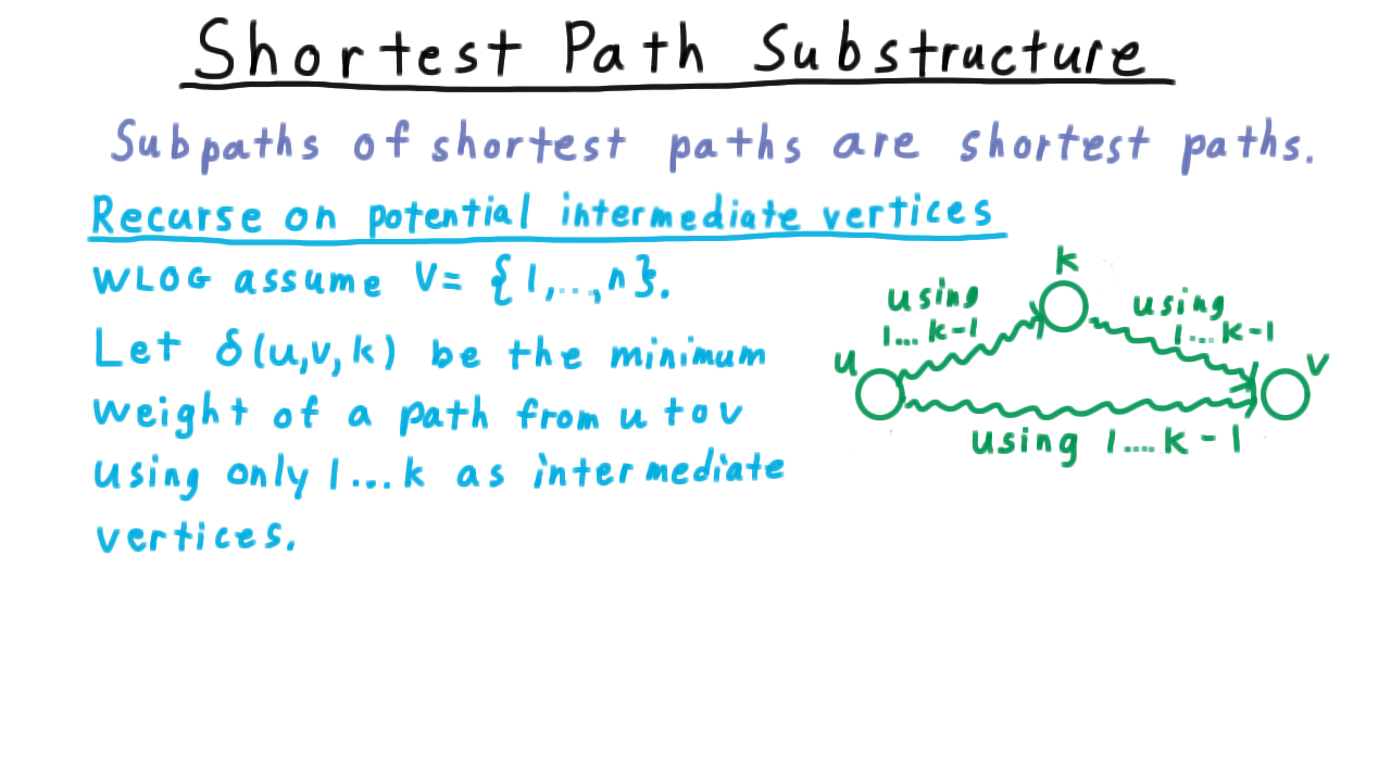
Therefore, we define \(\delta(u,v,k)\) to be the minimum weight of a path from \(u\) to \(v\) using only \(1\) through \(k\) as intermediate vertices.
Then the recurrence becomes
\[ \delta(u,v,k) = \min \{\delta(u,v,k-1), \delta(u,k,k-1) + \delta(k,v,k-1) \} \]
In the base case, where no intermediate vertices are allowed the weights and the edges provide all the needed information.
\[ \delta(u,v,0) = \left\{ \begin{array}{ll} w(u,v) & \mbox{ if }\; (u,v) \in E \\\\ 0 & \mbox{otherwise} \end{array} \right. \]
The Floyd-Warshall Algorithm - (Udacity, Youtube)
With this recurrence defined, we are now ready for the Floyd-Warshall Algorithm. Note that if we were to simply implement this with recursion, we would do a lot of recomputation. \(\delta(u,k,k-1)\) would be computed for every vertex \(v\) and \(\delta(k,v,k-1)\) would be computed for every vertex \(u.\)
As you might imagine, we are going to fill out a table. The subproblems have three indices, but thankfully only two will be required for us. We’ll create a two dimensional table \(d\) indexed by the source and destination vertices of the path. We initialize it for \(k=0,\) where no intermediate vertices are allowed.
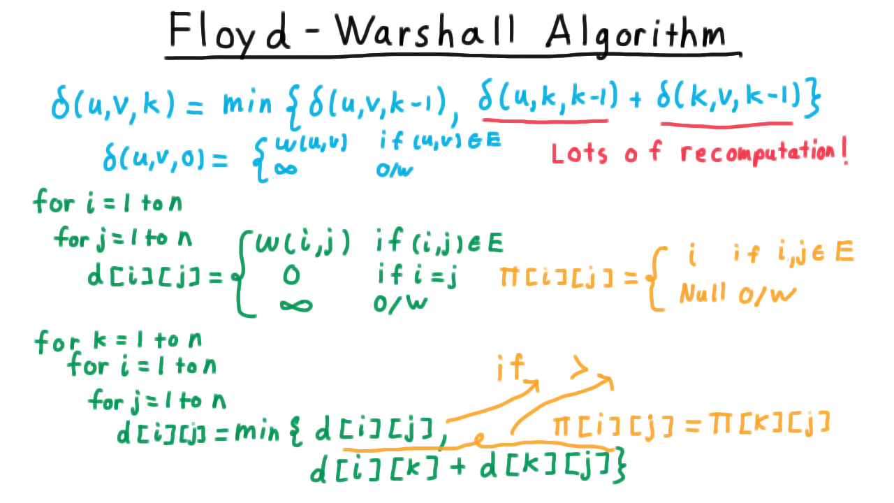
Then we allow the vertices one by one. For each source, destination pair, we update the weight of the shortest path accounting for the possibility of using k as an intermediate vertex. Note, that when \(i\) or \(j\) is equal to \(k\) the weight won’t change since a vertex can’t be useful in a shortest path to itself. Hence we don’t need to worry about using an outdated value in the loop.
To extract not just the weights of the shortest paths but also the paths themselves, we keep a predecessor table \(\pi\) that contains the second to last vertex on a path from \(u\) to \(v.\)
Initially, when all paths are single edges, this is just the other vertex on the incident edge. In the update phase, we either leave the predecessor alone if we aren’t change the path, or we switch it to the precessor of the k to j path if the path via k is preferable.
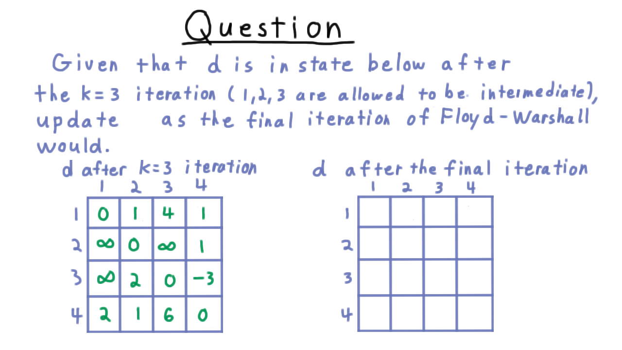
Floyd-Warshall Algorithm Exercise - (Udacity)
To check our understanding the Floyd-Warshall algorithm, let’s do an iteration as an exercise. Suppose that the table d is in the state below after the \(k=3\) iteration, which vertex 3 was allowed to be an intermediate vertex along a path, and I want you to fill in the table on the right with the values of d after the final iteration where k = 4.
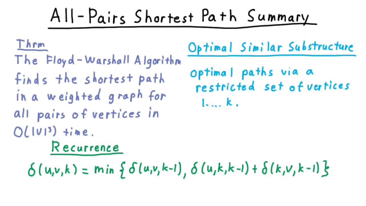
All Pairs Summary - (Udacity, Youtube)
Now, let’s summarize what we’ve shown about the All-Pairs shortest path problem. The Floyd-Warshall Algorithm, which is based on dynamic programming, finds the shortest path for all pairs of vertices in a weighted graph in time \(O(V^3).\) Recall that \(V\) times we have to fill out the whole table of size \(V^2\).
The key optimal similar substructure came from considering optimal paths via a restricted set of vertices \(1...k\)
That gave us the recurrence, where the shortest path between two vertices either used the new intermediate vertex, or it didn’t.
Transitive Closure - (Udacity, Youtube)
The Floyd-Warshall Algorithm has a neat connection to finding the transitive closure of mathematical relations. Consider a relation \(R\) over a set \(A.\) That is to say, \(R\) is a subset of \(A \times A.\) For example, \(A\) might represent sports that one can watch on television and the relation might be someone’s viewing preferences.
Maybe we know some individual prefers the NBA to college basketball and to college football and that he prefers college football to pro football. Since a relation is just a collection of ordered pairs, it makes sense to represent them as a directed graph.
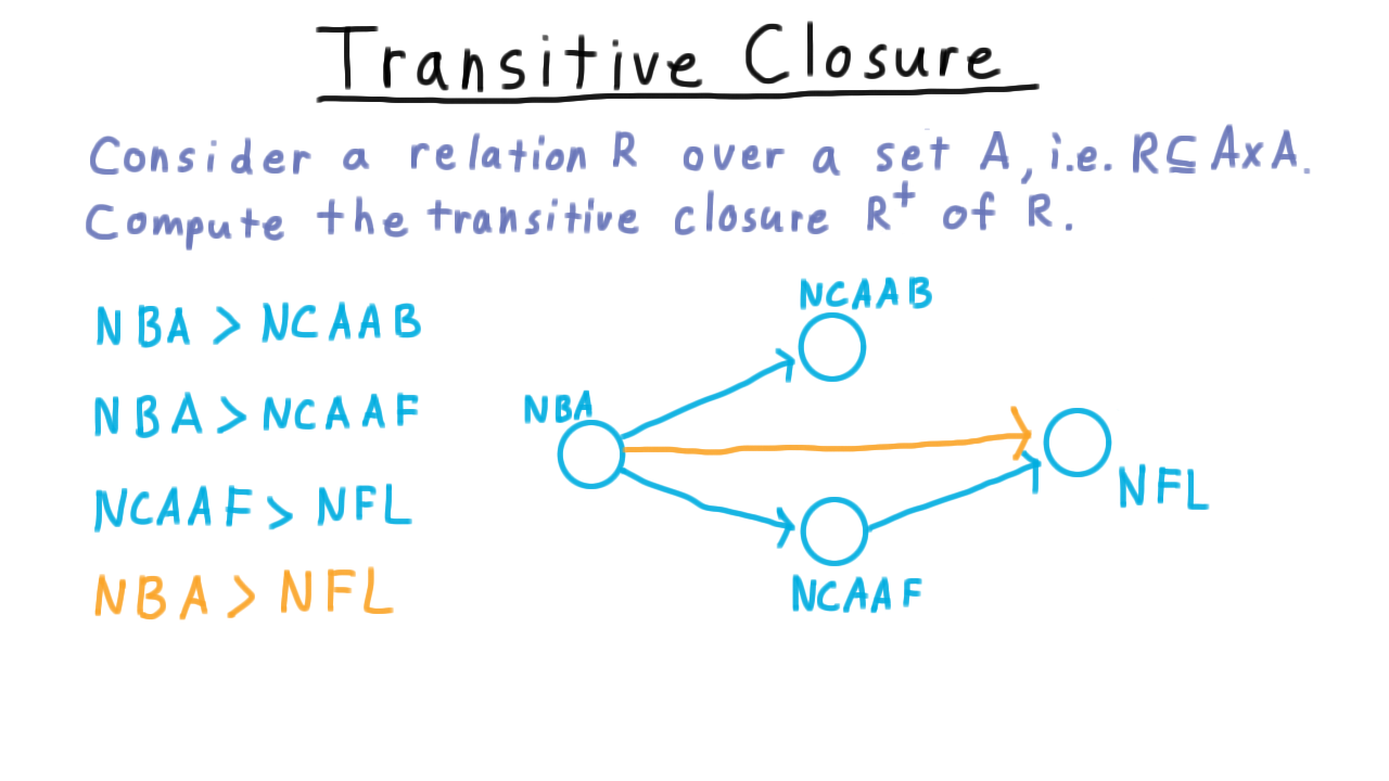
Given these preferences, we would like to be able to infer that this individual prefers the NBA over the NFL as well.
In effect, if there is a path from one vertex to another, we would like to add a direct edge between them. In set theory, this is called the transitive closure of a relation. Given what we know already, there is a fairly simple solution: just give each edge weight 1 and run Floyd-Warshall! The distance will be infinity if there is not path and it will minimum number of edges traversed otherwise.
This is more information that we really need, however. We really just want to know whether there is a path, not how long it is.
Hence, in this context we use a slight variant where the entries in the table are all booleans 0 or 1, instead of integers, but otherwise, the algorithm is essentially the same.
We initialize the table so that entry \(i,j\) is \(1\) if \((a_i,a_j)\) is in the relation and zero otherwise. Note that I’m letting \(a_1\) through \(a_n\) be the set \(A\) here. Then we keep on adding potential intermediary elements and updating the table accordingly. We have that \(i\) and \(j\) are in the relation if either they are in the relation already or they are linked together by \(a_k.\)
Often, we are interested not in the transitive closure of a relation but in the reflexive transitive closure. In this case, we just set the diagonal elements of the relation to be true from the beginning.
Conclusion - (Udacity, Youtube)
There are many other applications of dynamic programming that we haven’t touched on, but the three we covered provide a good sample, and help illustrate the general strategy. Perhaps, the most important lesson is that any time that you have found a recursive solution to a problem, think carefully about what the subproblems are and whether there overlap that you can exploit.
Note that this won’t always work. Dynamic programming will not create yield a polynomial algorithm for every problem with a recursive formulation. Take satisfiability for example. Pick a variable and set it to true and eliminate the variable from the formulation. We are left with another boolean formula, and if it’s satisfiable then so was the original. The same is true if we set the variable to false, and original formula will have a satisfying assignment if either of the other two do. This is a perfectly legitimate recursive formulation, yet there isn’t enough overlap between the problem to create a polynomial algorithm – at least, not unless P is equal to NP.
In the next lesson, we’ll examine the Fast Fourier Transform. This is much more a divide and conquer problem than it is a dynamic programming one, though many of the same themes of identifying subproblems and re-using calculation we appear as we study it. Keep this in mind as we study it.