Computability, Complexity, and Algorithms
Charles Brubaker and Lance Fortnow
Computability, Complexity, and Algorithms
Charles Brubaker and Lance Fortnow
Church-Turing Thesis - (Udacity)
Introduction - (Udacity, Youtube)
In this lecture, we will give strong evidence for the statement that
everything computable is computable by a Turing machine.
This statement is called the Church-Turing thesis, named for Alan Turing, whom we met in the previous lesson, and Alonzo Church, who had an alternative model of computation known as the lambda-calculus, which turns out to be exactly as powerful as a Turing machine. We call the Church-Turing thesis a thesis because it isn’t a statement that we can prove or disprove. In this lecture we’ll give a strong argument that our simple Turing machine can do anything today’s computers can do or anything a computer could ever do.
To convince you of the Church-Turing thesis, we’ll start from the basic Turing Machine and then branch out, showing that it is equivalent to machines as powerful as the most advanced machines today or in any conceivable future. We’ll begin by looking at multi-tape Turing machines, which in many cases are much easier to work with. And we’ll show that anything a multi-tape Turing machine can do, a regular Turing machine can do too.
Then we’ll consider the Random Access Model: a model capturing all the important capabilities of a modern computer, and we will show that it is equivalent to a multitape Turing machine. Therefore it must also be equivalent to a regular Turing machine. This means that a simple Turing machine can compute anything your Intel i7—or whatever chip you may happen to have in your computer—can.

Hopefully, by the end of the lesson, you will have understood all of these connections and you’ll be convinced that the Church-Turing thesis really is true. Formally, we can state the thesis as:
a language is “computable” if and only if it can be implemented on a Turing machine.
Simulating Machines - (Udacity, Youtube)
Before going into how single tape machines can simulate multitape ones, we will warm up with a very simple example to illustrate what is meant when we say that one machine can simulate another.
Let’s consider what I’ll call stay-put machines. These have the capability of not moving their heads in a computation step (which Turing machines, as we’ve defined them, are not allowed to do). So the transition function now includes S, which makes the head stay put. Now, this doesn’t add any additional computational capability to the machine, because I can accomplish the same things with a normal Turing machine. For every transition where the head stays put,
we can introduce a new state, and just have the head move one step right and then one step left. (Gamma here means match everything in the tape alphabet).

This puts the tape head back in the spot it started without affecting the tape’s contents. Except for occasionally taking an extra movement step, this Turing machine will operate in the same way as the stay-put machine.
More precisely, we say that two machines are equivalent
- if they accept the same inputs, reject the same inputs, and loop on the same inputs.
- considering the tape to be part of the output, equivalent machines also halt with the same tape contents.
Note that other properties of the machines (such as the number of states, the tape alphabet, or the number of steps in any given computation) do not need to be same. Just the relationship between the input and the output matters.
Multitape Turing Machines - (Udacity, Youtube)
Since having multiple tapes makes programming with Turing machines more convenient, and since it provides a nice intermediate step for getting into more complicated models, we’ll look at this Turing machine variant in detail. As shown in the figure here, each tape has its own tape head.

What the Turing machine does at each step is determined solely by its current state and the symbols under these heads. At each step, it can change the symbol under each head, and moves each head right or left, or just keeps it where it is. (With a one-tape machine, we always forced the head to move, but if we required that condition for multitape machines, the differences in tape head positions would always be even, which leads to awkwardness in programming. It’s better to allow the heads to stay put.)
Except for those differences, multitape Turing machines are the same as single-tape ones. We’ll only need to redefine the transition function. For a Turing machine with k tapes, the new transition function is
\[\delta: Q \times \Gamma^k : \rightarrow Q \times \Gamma^k \times \\{L,R,S\\}^k\]
Everything else stays the same.
Duplicate the Input - (Udacity, Youtube)
Let’s see a multitape Turing machine in action. Input always comes in on the first tape, and all the heads start at the left end of the tapes. Our task will be to duplicate this input, separated by a hash mark.

(See video for animation of the computation).
Substring Search - (Udacity)
Next, we’ll do a little exercise to practice using multitape Turing machines. Again, the point here is not so that you can put experience programming multitape Turing machines on your resume. The idea is to get you familiar with the model so that you can really convince yourself of the Church-Turing thesis and understand how Turing machines can interpret their own description in a later lesson.
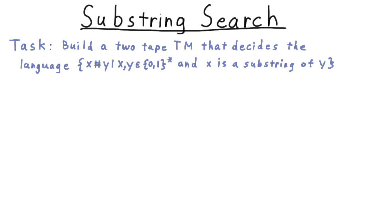
With that in mind, your task is to build a two-tape TM that decides the language strings of the form x#y, where x is a substring of y. So for example, the string 101#01010 is in the language.
The second through fourth character of y match x. But on the other hand, 001#01010 is not in the language. Even though two 0s and a 1 appear in the string 01010, 001 is not a substring because the numbers are not consecutive.
Multitape SingleTape Equivalence - (Udacity, Youtube)
Now, I will argue that these enhanced multitape Turing machines have the same computational power as regular Turing machines. Multitape machines certainly don’t have less power: by ignoring all but the input tape, we obtain a regular Turing machine.
Let’s see why multitape machines don’t have any more power than regular machines.
On the left, we have a multitape Turing machine in some configuration, and on the right, we have created a corresponding configuration for a single-tape Turing machine.

On the single tape, we have the contents of the multiple tapes, with each tape’s contents separated by a hash. Also, note these dots here. We are using a trick that we haven’t used before: expanding the size of the alphabet. For every symbol in the tape alphabet of the multitape machine, we have two on the single tape machine, one that is marked by a dot and one that is unmarked. We use the marked symbols to indicate that a head of the multitape machine would be over this position on the tape.
Simulating a step of the multitape machine with the single tape version happens in two phases: one for reading and one for writing. First, the single-tape machine simulates the simultaneous reading of the heads of the multitape machines by scanning over the tape and noting which symbols have marks. That completes the first phase where we read the symbols.
Now we need to update the tape contents and head positions or markers as part of the writing phase. This is done in a second, leftward pass across the tape. (See video for an example.)
Note that it is possible that one of these strings will need to increase its length when the multitape reaches a position it hasn’t reached before. In that case, we just right-shift the tape contents to allow room for the new symbol to be written.
Once all that work is done, we return the head back to the beginning to prepare for the next pass.
So, all the information about the configuration of a multitape machine can be captured in a single tape. It shouldn’t be too hard to convince yourself that the logic of reaching and keeping track of the multiple dotted symbols and taking the right action should be as well. In fact, this would be a good for you to do on your own.
Analysis of Multitape Simulation - (Udacity)
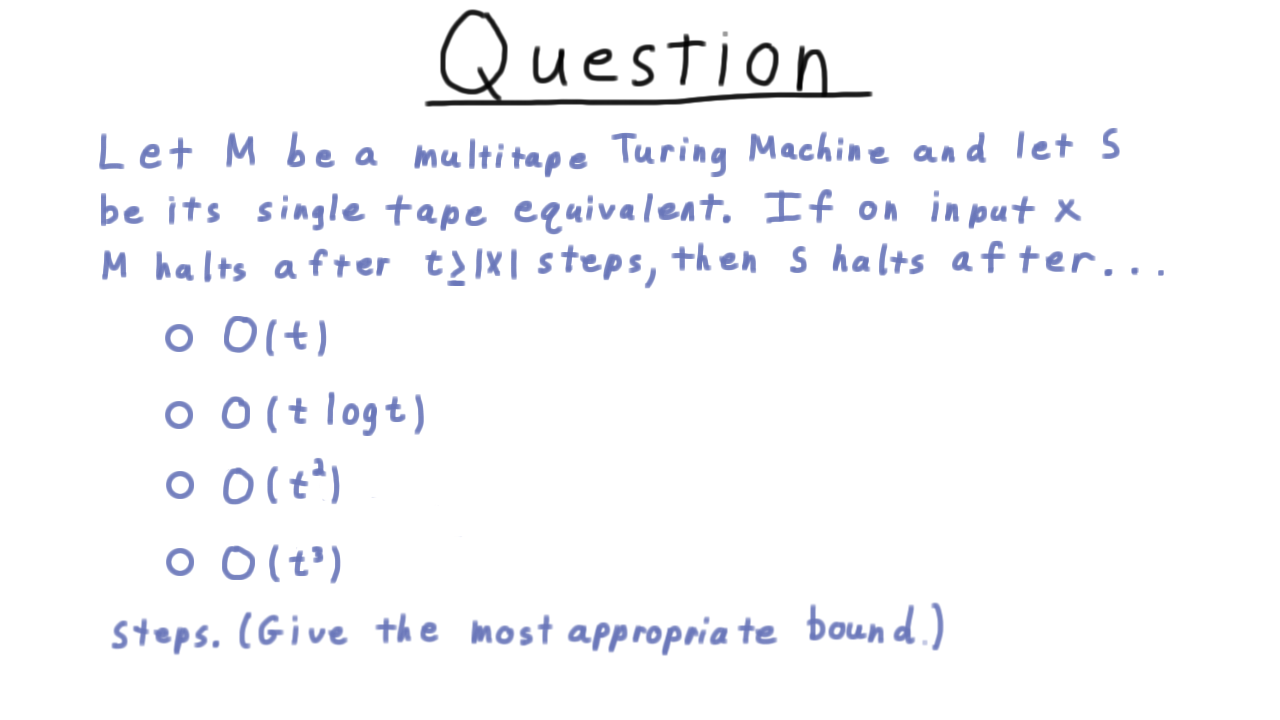
Now for an exercise. No more programming Turing machines. Instead, I want you to try to figure out how long this simulation process takes. Let M be a multitape Turing machine and let S be its single-tape equivalent as we’ve defined it. If on input x, M halts after t steps, then S halts after… how many steps. Give the most appropriate bound. Note that we are treating the number of tapes k as a constant here.
This question isn’t easy, so just spend a few minutes thinking about it and take a guess, before watching the video answer.
RAM Model - (Udacity, Youtube)
There are other curious variants of the basic Turing machines: we can restrict them so that a symbol on a square can only be changed once, we can let them have two-way infinite tapes, or even let them be nondeterministic (we’ll examine this idea when we get to complexity). All of these things are equivalent to Turing machines in the sense we have been talking about, and it’s good to know that they are equivalent.
Ultimately, however, I doubt that the equivalence of those models does much to convince anyone that Turing machines capture the common notion of computation. To make that argument, we will show that a Turing machine is equivalent to the Random Access model, which very closely resembles the basic CPU/register/memory paradigm behind the design of modern computers.
Here is a representation of the RAM model.

Instead of operating with a finite alphabet like a Turing machine, the RAM model operates with non-negative integers, which can be arbitrarily large. It has registers, useful for storing operands for the basic operations and an infinite storage device analogous to the tape of a regular Turing machine. I’ll call this memory for obvious reasons. There are two key differences between this memory and the tape of a regular Turing machine:
- each position on this device stores a number an
- any element can be be read with a single instruction, instead of moving a head over the tape to the right spot.
In addition to this storage, the machine also contains the program itself expressed as a sequence of instructions and a special register called the program counter, which keeps track of which instruction should be executed next. Every instruction is one of a finite set that closely resembles the instructions of assembly code. For instance, we have the instruction read j, which reads the contents from the jth address on the memory and places it in register 0. Register 0, by the way, has a special status and is involved in almost every operation. We also have a write operation, which writes to the jth address in memory. For moving data between the registers, we have load, which write to \(R_0\), and store which writes from it, as well as add, which increases the number in \(R_0\) by the amount in \(R_j\). All of these operations cause the program counter to be incremented by 1 after they are finished.
To jump around the list of instructions—as one needs to do for conditionals—we have a series of jump instructions that change the program counter, sometimes depending on the value in \(R_0\).
And finally, of course, we have the halt instruction to end the program. The final value in \(R_0\) determines whether it accepts or rejects. Note that in our definition here there is no multiplication. We can achieve that through repeated addition.
We won’t have much use for the notation surrounding the RAM model, but nevertheless it’s good to write things down mathematically, as this sometimes sharpens our understanding. In this spirit, we can say that a Random Access Turing machine consists of :
- a natural number \(k\) indicating the number of registers
- and a sequence of instructions \(\Pi\).
The configuration of a Random Access machine is defined by
- the counter value, which is 0 for the halting state and indicates the next instruction to be executed otherwise.
- the register values and the values in the memory, which can be expressed as a function.
(Note that only a finite number of the addresses will contain a nonzero value, so this function always has a finite representation. We’ll use 1-based indexing, hence the domain for the tape is the natural numbers starting from one.)
Equivalence of RAM and Turing Machines - (Udacity, Youtube)
Now we are ready to argue for the equivalence of our Random Access Model and the traditional Turing machine. To translate between the symbol representation of the Turing machine and numbers of RAM, we’ll use a one-to-one correspondence E.
The blank symbol is mapped to to zero (\(E(\sqcup) = 0)so that the default value of the tape corresponds to the default value for memory.
First, we argue that a RAM can simulate a single tape Turing machine. The role of the tape played in the Turing machine will be played by the memory We'll keep track of the head position in a fixed register, say \)R_1\(. And the program and the program counter will implement the transition function. Here, I've written out in pseudocode what this might look like for the simple Turing machine shown over here, which just replaces all the ones with zeros and then halts.

Now we argue the other way: that a traditional Turing machine can simulate a RAM. Actually, we’ll create a multitape Turing machine that implements a RAM since that is a little easier to conceptualize. As we’ve seen, anything that can be done on a multitape Turing machine can be done with a single tape.

We will have one tape per register, and each tape will represent the number stored in the corresponding register.
We also have another tape that is useful for scratch work in some of the instructions that involve constants like add 55.
Then we have two tapes corresponding to the random access device. One is for input and output, and the other is for simulating the contents of the memory device during execution. Storing the contents of the random access device is the more interesting part. This is done just by concatenating the (index, values) pairs using some standard syntax like parentheses and commas.
The program of the RAM must be simulated by the state transitions of the Turing machine. This can be accomplished by having a subroutine or sub-Turing machine for each instruction in the program. The most interesting of these instructions are the ones involving memory. We simulate those by searching the tape that stores the contents of the RAM for one of these pairs that has the proper index and then reading or writing the value as appropriate. If no such pair is found, then the value on the memory device must be zero.
After the work of the instruction is completed, the effect of incrementing the program counter is achieved by transitioning to the state corresponding to the start of the next instruction. That is, unless the instruction was a jump, in which case that transition is effected. Once the halt instruction is executed the contents of the tape simulating the random access device are copied out onto the I/O tape.
RAM Simulation Running Time - (Udacity)
Given this description about how a traditional Turing machine can simulate a Random Access Model, I want you to think about how long this simulation takes. Let R be a random access machine and let M be its multi-tape equivalent. We’ll let n be the length of the binary encoding of the input to R and let t be the number of steps taken by R. Then M takes how long to simulate R?
This is a tough question, so I’ll give you a hint: the length of the representation of a number increases by at most a constant in each step of the random access machine R.

Conclusion - (Udacity, Youtube)
Once you know that a Turing machine can simulate a RAM, then you know it can simulate a standard CPU. Once you can simulate a CPU, you can simulate any interpreter or compiler and thus any programming language. So anything you can run on your desktop computer can be simulated by a Turing machine.
What about multi-core, cloud computing, probabilistic, quantum and DNA computing? We won’t do it here, but you can prove Turing machines can simulate all those models as well. The Church-Turing thesis has truly stood the test of time. Models of computation have come and go but none have been any match for the Turing machine.
Why should we care about the Church-Turing thesis? Because there are problems that Turing machines can’t solve. We argued this with counting arguments in the first lecture and will give specific examples in future lectures. If these problems can’t be solved by Turing machines they can’t be solved by any other computing device.
To help us describe specific problems that one cannot compute, in the next lecture we discuss two of Turing’s critical insights: that a computer program can be viewed as data—as part of the input to another program—and that one can have a universal Turing machine that can simulate the code of any other computer: one machine to rule them all.