Computability, Complexity, and Algorithms
Charles Brubaker and Lance Fortnow
Computability, Complexity, and Algorithms
Charles Brubaker and Lance Fortnow
Bipartite Matching - (Udacity)
Introduction - (Udacity, Youtube)
In this lesson, we’ll discuss the problem of finding a maximum matching in a bipartite graph, a problem intimately related to finding a maximum flow in a network. Indeed, our initial algorithm will come from a reduction to max flow, and at first, maximum bipartite matching might seem just like a special case. As we examine the problem more carefully, however, we’ll see some special structure, and eventually, we will use this insight to create a better algorithm.
Bipartite Graphs - (Udacity, Youtube)
We begin our discussion by defining the notion of a bipartite graph.
An undirected graph is bipartite if there is a partition of the vertices L and R (think of these as left and right) such that every edge has one vertex in L and one in R. For example, this graph here is bipartite.

I can label the green vertices as L and the orange ones as R, and every edge is between a green and an orange vertex.
A few observations are in order. First, saying the a graph is bipartite is equivalent to saying that it is two-colorable for those familiar with colorings.
Next, let’s take this same graph and add this edge here to make it non-bipartite.

Note that I’ve introduced an odd-length cycle, and indeed saying that a graph is bipartite is equivalent to saying that it has no odd-length cycles.
For graphs that aren’t connected it’s possible that there will be some ambiguity in the partition of the vertices, so sometimes the partition is included in the definition of the graph, as in \(G=(L,R,E)\).
Bipartite Graph Quiz - (Udacity)
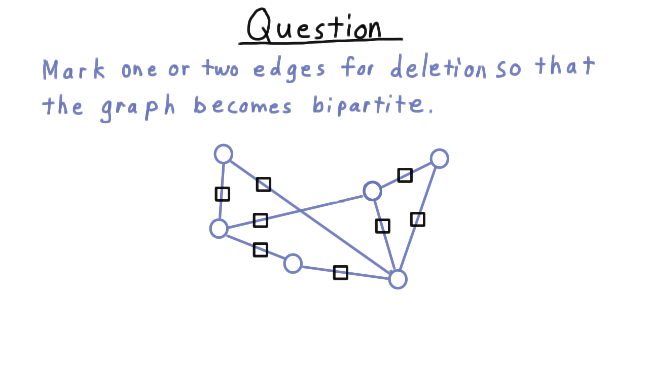
Here is a quick exercise on bipartite graphs. I’ve drawn a graph here that it not bipartite, and I want you to select one or two edges for deletion so that it become bipartite.
Matching - (Udacity, Youtube)
Our next important concept is the matching.
Given a graph, a subset of the edges is a matching if no two edges share (or are incident on) the same vertex.
Note that the graph doesn’t have to be bipartite. Take for example, this graph here.
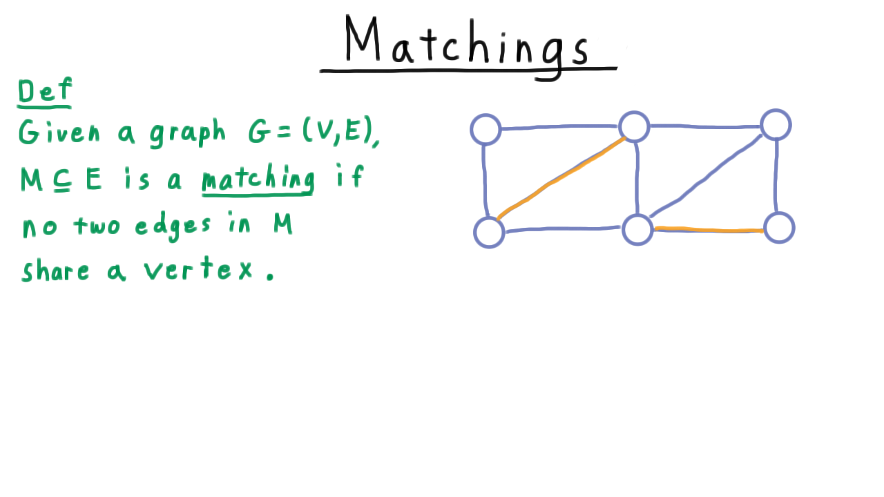
These two edges marked in orange constitute a matching. By the way, we’ll refer to an edge in a matching as a matched edge, so these two edges are matched, and we’ll refer to a vertex in a matched edge as a matched vertex. Here, there are four matched vertices.
A maximum matching is a matching of maximum cardinality.
Note that a maximal matching is not a maximum matching. For instance, the shown above is maximal because I can’t add any more edges and have it still be a matching. On the other hand, it is not maximum because here is a matching that has greater cardinality.

This happens in bipartite graphs too. It is possible to have a maximal matching that is not maximum because there is a greater matching.
Applications - (Udacity)
Now that we know what bipartite graphs and matchings are, let’s consider where the problem of finding a maximum matching in a bipartite graph comes up in real-world applications. Actually, we’ll make this a quiz where I give you some problem descriptions and you tell me which can be cast as maximum matching problems in bipartite graphs.
First consider the compatible roommate problem. Here some set of individuals give a list of habits and preferences and for each pair we decide if they are compatible. Then we want to match roommates so as to get a maximum number of compatible roommates.
Next, consider the problem of assigning taxis to customers so as to minimize total pick-up time.
Another application is assigning professors to classes that they are qualified to teach. Obviously, we hope to be able to offer all of the classes we want.
And lastly, consider matching organ donors to patients who are likely to be able to accept the transplant. Of course, we want to be able to do as many transplants as possible.
Check all the applications that can naturally cast as a maximum matching problem.

Reduction to Max Flow - (Udacity, Youtube)
At this point, we’ve defined a bipartite graph and the notion of a matching. Now we are going see the connection with maximum flow.
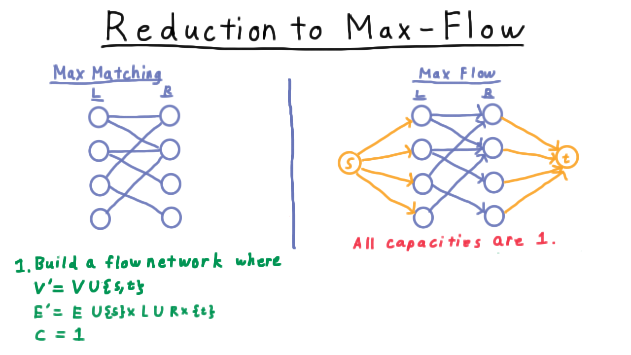
Intuitively, a maximum matching problem should feel like we are trying to push as much stuff from one side of the partition to the other. It should be no surprise then that there turns out to be an easy reduction to the maximum flow problem, which we’ve already studied.
We build a flow network that has the same set of vertices, plus two more which serve as the source and the sink. We then add edges from the source to one half of the partition and edges from the other half of the partition to the sink. Edges are given a direction from the source side to the sink side. All the capacities are set to 1. Setting the capacities of the new edges to 1 is important to ensure that the flow from or to any vertex isn’t more than 1.
Having constructed the graph, we then run Ford-Fulkerson on it,
and we return the the edges with positive flows as the matching. Actually, all edges will have flows 0 or 1 as we’ll see.
The time analysis here is rather simple. Building the network is \(O(E)\) maybe \(O(V)\) depending on the representation used.
This is small, however, compared to the cost of running Ford-Fulkerson which is \(O(EV).\) Note that \(V\) is a bound on the total capacity of the flow and hence a bound on the total number of iterations. In this particular case, this gives a better bound than given by the scaling algorithm or by Edmonds-Karp.
Lastly, of course, returning the matched edges is just a matter of saying for each vertex on the left, which vertex on the right does it send flow to. That’s just \(O(V)\) time.
Clearly, Ford-Fulkerson is the dominant part and we end up with an algorithm that runs in time \(O(EV).\)

Reduction Correctness - (Udacity, Youtube)
We assert the correctness of the reduction with following theorem…
Consider a bipartite graph \(G\) and the associated flow network \(F\). The edges of \(G\) which have flows of 1 in a maximum flow obtained by Ford-Fulkerson on \(F\) constitute a maximum matching in \(G.\)
To prove this theorem, we start by observing that the flow across any edge is either zero or one. Any augmenting path, will have a bottleneck capacity of 1, so we’ll always augment flows by 1, but 1 is also the maximum flow that can flow across any edge.
The conservation of flow then implies that each vertex is in at most 1 edge of that we return. On the left, hand side, we only have one unit of capacity going in, so we can’t have more than one unit of flow going out. On the right we have only, one unit of capacity going out so we can’t have more than one unit of flow going in. This means that the set of edges in the original graph that have flow 1 represent a matching.
Is it a maximum matching? Well, if there were are larger matching it would be trivial to construct a larger flow just by sending flow along those edges, so yes it must be a maximum matching.
Deeper Understanding - (Udacity, Youtube)
At this point, it’s tempting to be satisfied with the result. After all, we have found a relatively low-order polynomial solution for problem.
On the other hand, the sort of flow networks we are dealing with here are very specialized, having all unit capacities and a bipartite structure. Our algorithm doesn’t exploit this at all.
In the remainder of the lecture, we’ll look at this special structure more closely, gain some additional insights about bipartite matchings, and finally these will lead us to a faster algorithm.
Augmenting Paths - (Udacity, Youtube)
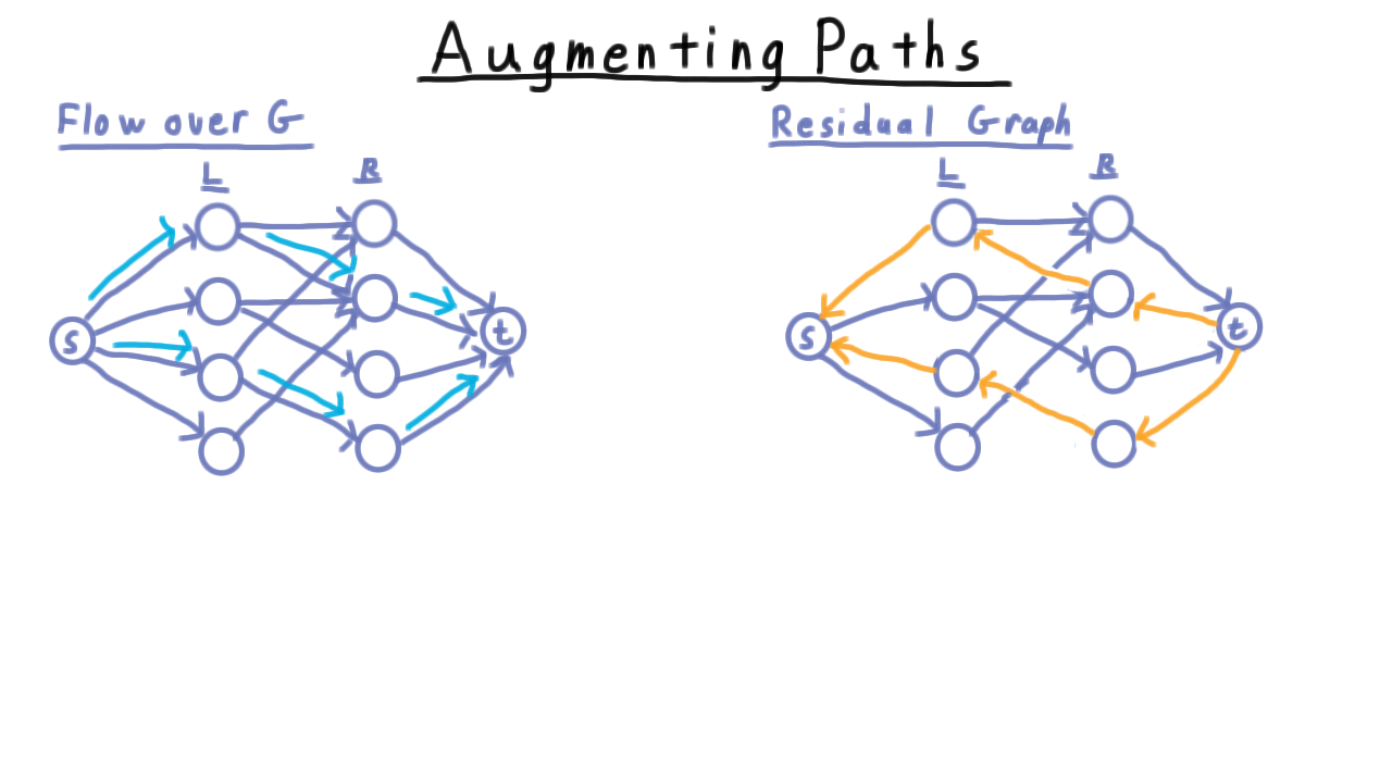
We start this search for a deeper understanding with the augmenting path. Recall that in our treatment of the maximum flow problem, we were given a flow over some graph and we defined the residual network, which captured the ways in which we were allowed to modify this flow. This included adding backwards edges that went in to opposite of the direction from edges in the original graph. Augmenting paths then were paths over this residual network from the source to the sink that increased (or augmented) the flow.

In a network that arises from a bipartite matching problem, there are a few special phenomena that are worth noting. First, observe that all intermediate flows found by Ford-Fulkerson correspond to matchings as well. If there is flow across an internal edge, then it belongs in the matching.
Also, because flows along the edges are either 0 or 1, there are no antiparallel edges in the residual network. That is to say that either the original edge is there or the reverse is, never both. Moreover, the matched edges are the ones that have their direction reversed. Also, only unmatched vertices have an edge from the source or to the sink. Matched vertices have these edges reversed.
The result of all of this is that any augmenting path must start at an unmatched vertex and then alternately follow an unmatched, then a matched edge, then an unmatched edge, and so forth until it finally reaches an unmatched vertex on the other side of the partition.
This realization allows us to strip away much of the complexity of flow networks and define an augmenting path for a bipartite matching in more natural terms.
We start by defining the more general concept of an alternating path.
Given a matching \(M\) an alternating path is one where the edges are alternately in \(m\) and not in \(M\). An augmenting path is an alternating path where the first and last edges are unmatched.
For example, the path shown in blue on the right is an augmenting path for the matching illustrated in purple on the left.

We use it to augment the matching by making the unmatched edges matched and the matched ones matched along this path. This always increases the size of the matching because before we flipped there was one more unmatched edge than matched edge along the path, so when we reverse the matched and unmatched edges, we increase the size of the matching by one.
In fact, we can restate the Ford-Fulkerson method purely in these terms.
- Initialize \(M = \emptyset.\)
- While there is an augmenting math \(p\), update \(M = M \oplus p\).
- Return \(M.\)
(Here the \(\oplus\) operator denotes the symmetric difference. I.e. \(A \oplus B = (A \cup B) - (A \cap B).\))
Vertex Cover - (Udacity, Youtube)
Now we turn to the concept of a vertex cover, which will play a role analogous to the one played by the concept a minimum cut in our discussion of maximum flows.
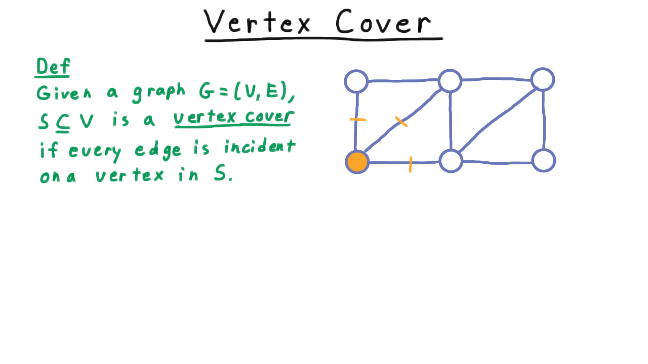
Given a graph \(G=(V,E),\) \(S \subseteq V\) is a vertex cover if every edge is incident on a vertex in S.
We also say that \(S\) covers all the edges. Take this graph, for example. If we include the lower left vertex marked in orange, then we cover three edges.
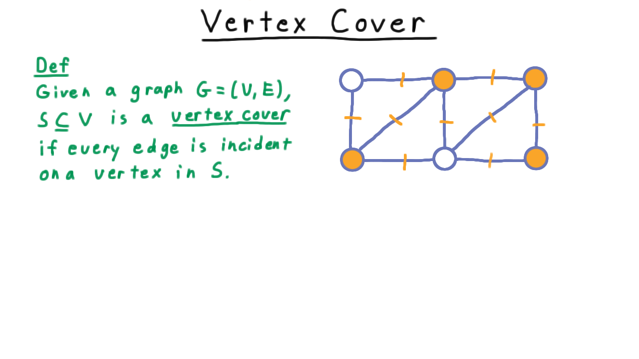
By choosing more vertices so as to cover more edges, we might end up with a cover like this one.
One pretty easy observation to make about a vertex cover is that it’s size serves as an upper bound for the size a matching in the graph.
In any given graph, the size of a matching is at most the size of a vertex cover.
The proof is simple. Clearly, for every edge in the matching at least one vertex must be in the cover, and all of these vertices must be distinct because no vertex is in two matched edges.
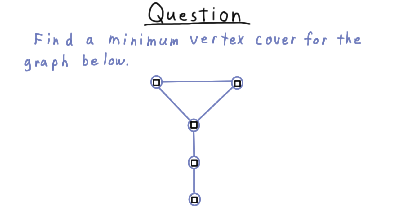
Find a Min Vertex Cover - (Udacity)
Let’s get a little practice with vertex covers. Find a minimum vertex cover (i.e. one of minimum cardinality) for the graph below.
Max Matching Min Vertex Cover - (Udacity, Youtube)
Now, we are ready for the matching equivalent of the maxflow/mincut theorem, the max-matching/min vertex cover theorem.
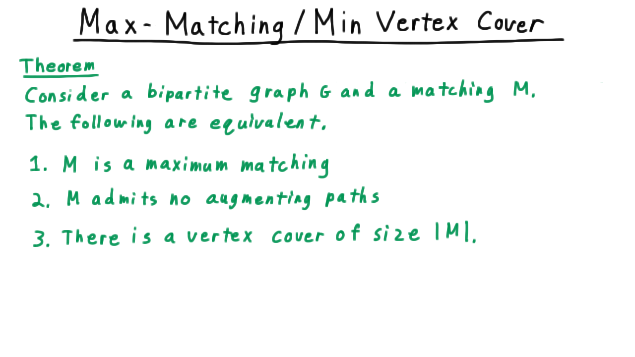
The proof is very similar. We begin by showing that if \(M\) is a matching then it admits no augmenting paths. Well, suppose not. Then there is some augmenting path, and if we augment \(M\) by this path, we get a larger matching, meaning that \(M\) was not a maximum as we had supposed.
Next, we argue that if \(M\) admits no augmenting paths. Then we claim that there there exists a vertex cover of the same size as \(M.\) This is the most interesting part of the proof. We’ll let \(H\) be the set of vertices reachable via an alternating paths from unmatched vertices in \(L\) (the left hand side of the partition).
We can visualize this definition by starting with some unmatched vertices in L, then following it’s edges to some set in R, then including it’s the vertices in L that these are matched with, etc.
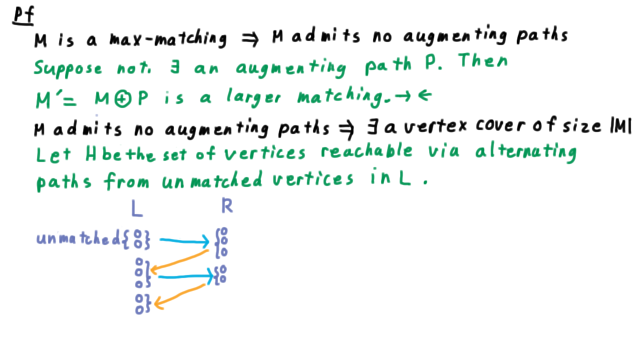
Note that because, \(M\) doesn’t admit any augmenting paths, all of these paths must terminate in some matched vertex in \(L.\) Let’s draw the rest of the graph here as well.
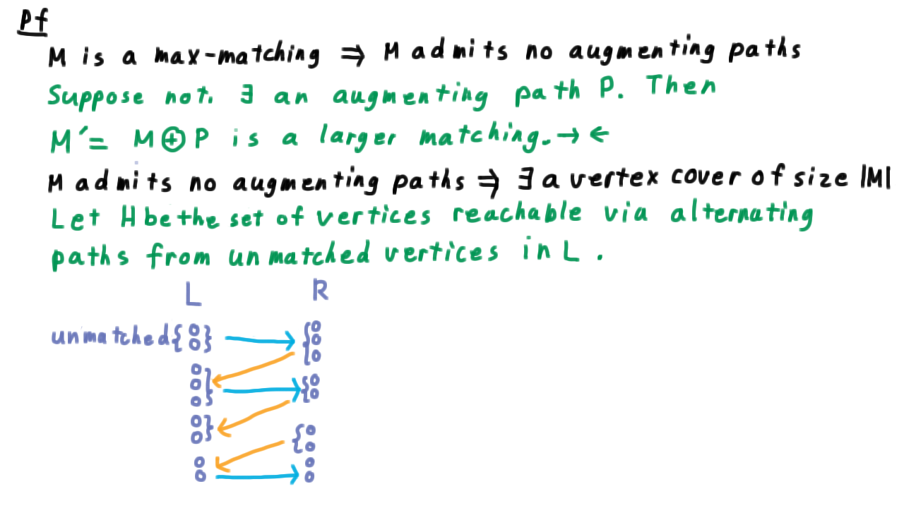
We have some matched vertices in \(L,\) the vertices in \(R\) that they are matched to, and some unmatched vertices in \(R.\) Note that \(H\) and \(\overline{H}\) correspond to the minimum cut we used when discussing flows. To get a min vertex cover, we select the part of \(H\) that is in \(R\) and the part of \(L\) that is not.

We call this set \(S.\) This set \(S\) contains exactly one vertex of each edge in \(M,\) so \(|S| = |M|.\)
Next, we need to convince ourselves that \(S\) is really a vertex cover. The edges we need to worry about are those from \(L \cap H\) to \(R-H\). Such an edge cannot be matched by our definition, and any such unmatched edge would place the vertex in \(R\) into \(H\). Therefore, there are no such edges and S is a vertex cover.
Finally, we have to prove that the existence of a vertex cover that is the same size as a matching implies that the matching is a maximum. This follows immediately from our discussion that a vertex cover is an upper bound of the size of a matching.
The Frobenius-Hall Theorem - (Udacity, Youtube)
Before we turn to finding a faster algorithm for finding a max matching, there is a classic theorem related to matchings that we should talk about. This is the Frobenius-Hall theorem. For a subset of the vertices \(X,\) we’ll use \(N(X)\) to indicate the union of the neighbors of the individual vertices in \(X.\)
If we consider this graph here, then the neighbors of the orange vertices will be the green ones.
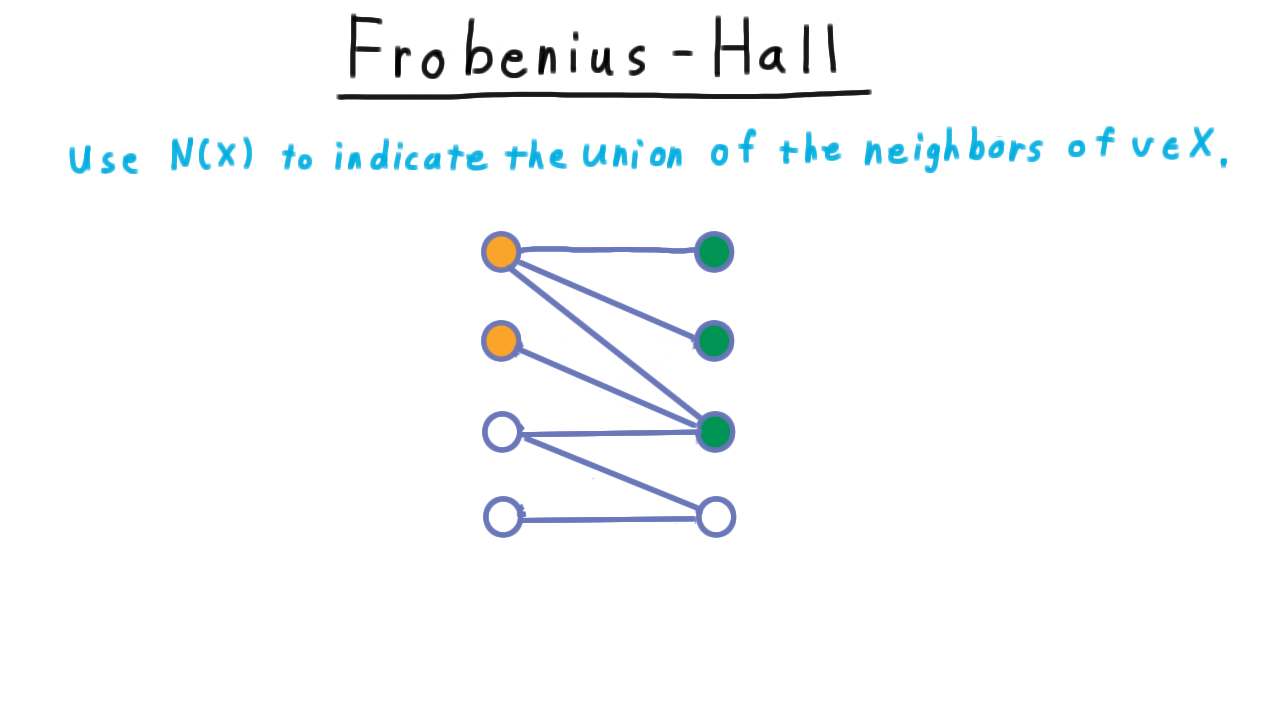
Note that the fact that the neighborhood of X is larger than X bodes well for the possibility of finding a match for all the vertices on the left hand side. At least, there is a chance that we will be able to find a match for all of these vertices.
When this is not the case, as seen below, then it is hopeless.

Regardless of how we match the first two, there will be no remaining candidates for the third vertex.
We can make this intuition precise with the Frobenius-Hall Theorem which follows from the max-matching/min vertex cover argument.
Given a bipartite graph \(G = (L,R,E)\), there is a matching of size \(|L|\) if and only if for every \(X \subseteq L\), we have that \(|N(X)| \geq |X|.\)
The forward direction is the simpler one. We let \(M\) be a matching of the same size as the left partition, let \(X\) be any subset of this side of the partition, and we let \(Y\) be the vertices that \(X\) is matched to.
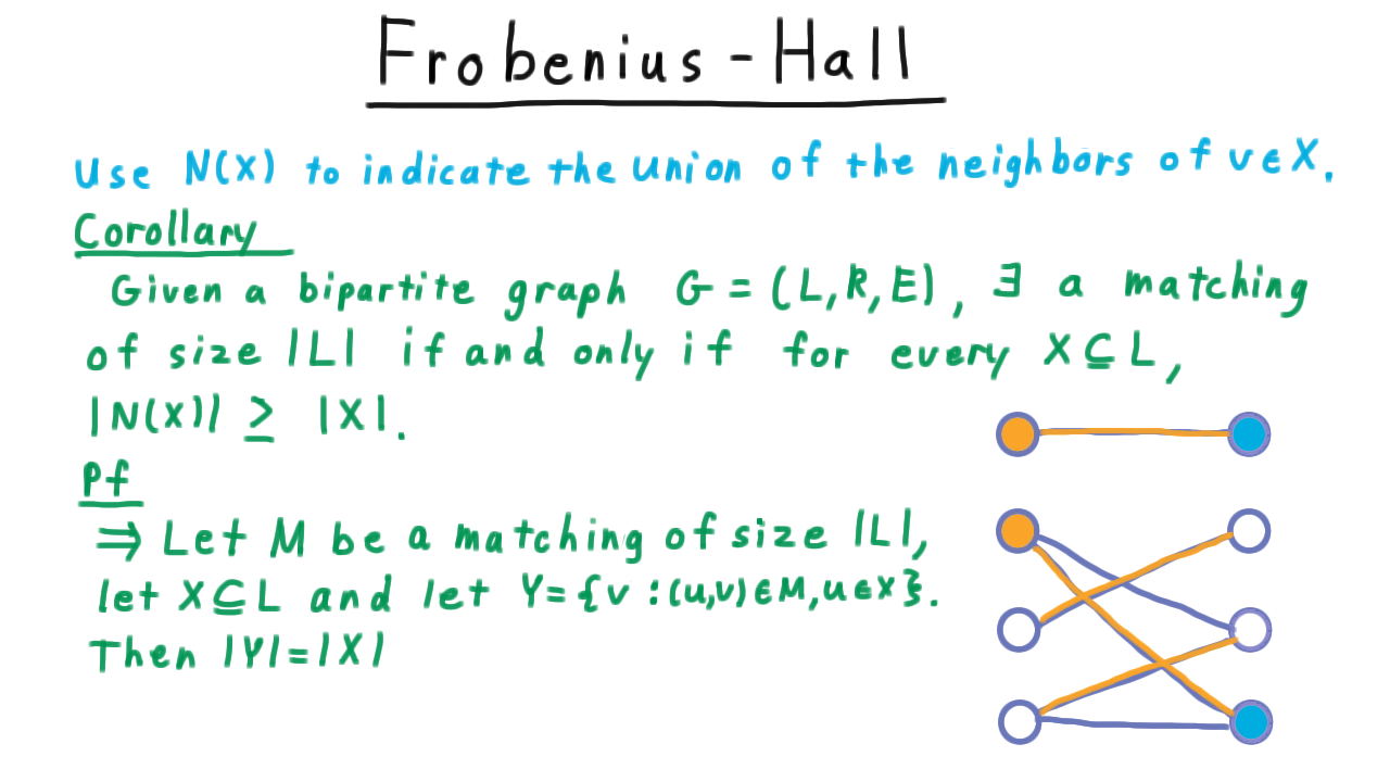
Because the edges of the matching don’t share vertices, \(|Y|=|X|.\) Yet, \(Y\subseteq N(X),\) implying that \(|X| = |Y| \leq |N(X)|.\)neighborhood of X is at least the size of X.
The other direction is a little more challenging. Suppose not. That is, there is a maximum matching \(M,\) and it has fewer than \(|L|\) edges. We let \(H\) be the set of vertices reachable via an alternating path from an unmatched vertex in \(L.\) This is the same picture used in the max-matching/min-vertex cover argument. There is at least one such unmatched vertex by our assumption here.
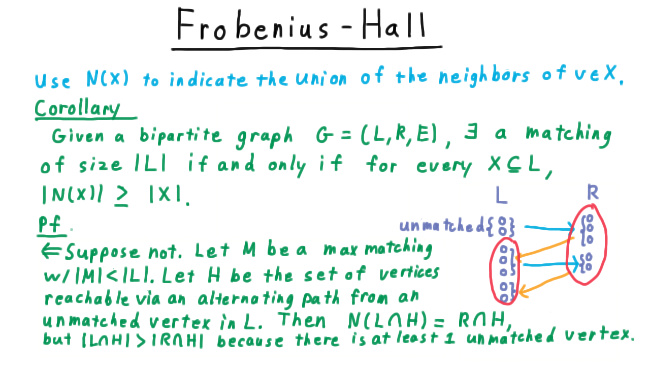
The neighborhood of the left side of \(H\) is just the right side of \(H\) by construction, but the left hand side must be strictly larger, because the matched vertices on either side effectively cancel each other out, leaving the unmatched vertices in \(L\) as extras.
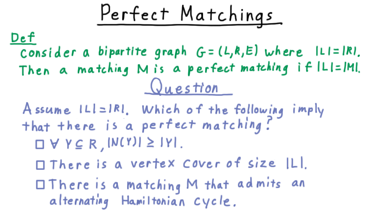
Perfect Matchings - (Udacity)
Our treatment of matchings wouldn’t be complete without talking about the notion of a perfect matching.
In a bipartite graph \(G=(L,R,E))\) a matching \(M\) is perfect if \(|M|=|L|=|R|.\)
That is to say all of the vertices are matched. To review some of the key concepts from the lesson so far, we’ll do a short exercise. Assume that the left and right sides are of the same size. Which of the following implies that there is a perfect matching?
Toward a Better Algorithm - (Udacity, Youtube)
Now that have a deeper understanding of the relationship between max-matching and max-flow problems, we are ready to understand a more sophisticated algorithm. Back in the maximum-flow lecture we considered two ways to improve over the naive Ford-Fulkerson. One was to prefer heavier augmenting paths, ones that pushed more flow from the source to the sink. In the max-matching context this doesn’t make much sense because all augmenting path have the same effect, they increase the matching by one.
The other idea was to prefer the shortest augmenting paths and there was Dinic’s further insight that the breadth first search need only be done when the shortest path length changed, not once for every augmentation. Pursuing these ideas gives us the Hopcroft Karp algorithm.
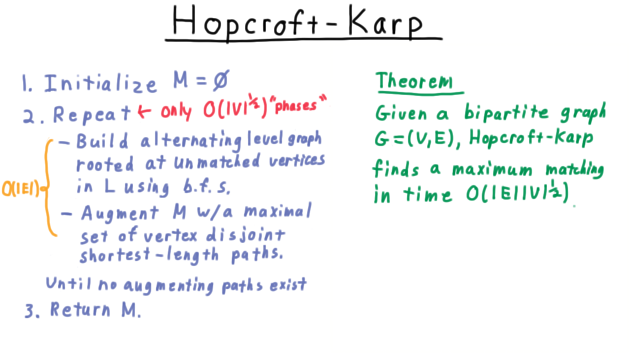
The Hopcroft-Karp Algorithm - (Udacity, Youtube)
The Hopcroft-Karp algorithm goes like this.

We first initialize the matching to the empty set. Then we repeat the following: first build an alternating level graph rooted at the unmatched vertices in the left partition L, using a breadth-first-search. Here the original graph is shown on the left and the associate level graph on the right.
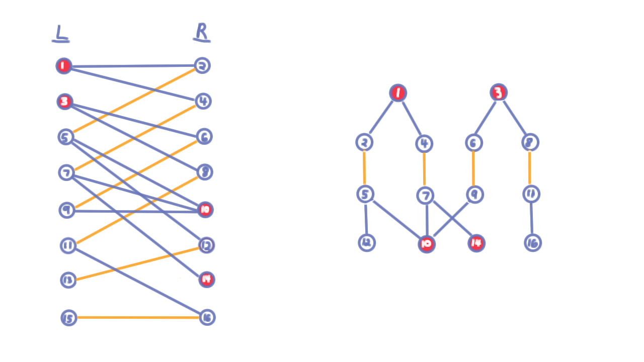
Having built this level graph, we use it augment the current matching with a maximal set of vertex-disjoint shortest augmenting paths.
We accomplish this by starting at the the unmatched vertex in \(R\) and tracing our way back. Having found a path to an unmatched vertex in \(R\), we delete the vertices along the path as well as any orphaned vertices in the level graph. (See the video for an example.)
Note that we only achieve a maximal set of vertex-disjoint paths here, not a maximum. Once we have applied all of these augmenting paths, we go back an rebuild the level graph and keep doing this until no more augmenting paths are found. At that point we have found a maximum matching and we can return \(M.\)
From the description, it is clear that each iteration in this loop–what we call a phase from now on–takes only \(O(E)\) time. The first part is accomplished via bread-first-search and the second also amounts to just a single traversal of the level graph.
The key insight is that only about the \(\sqrt{V}\) phases are needed.
Our overall goal, then is to proof the theorem stated in the figure below.
Matching Differences - (Udacity)
Our first step is to understand the difference between the maximum matching that the algorithm finds and the intermediate matchings that the algorithm produces along the way. Actually, we’ll state key claim in terms of two arbitrary matchings \(M\) and \(M'\)
and I want you to help me out. Think about the graph containing edges that are in \(M\) but not in \(M'\) or vice-versa and tell me which of the following statements are true.
(Watch the answer on the Udacity site)
The key result is the following.
If \(M^*\) is a maximum matching and \(M\) is another matching, then \(M^* \oplus M\) contains \(|M^*|- |M|\) vertex-dsijoint paths that augment \(M.\)
Shortest Augmenting Paths - (Udacity, Youtube)
This next lemma will characterize the effect of choosing to augment by a shortest path.
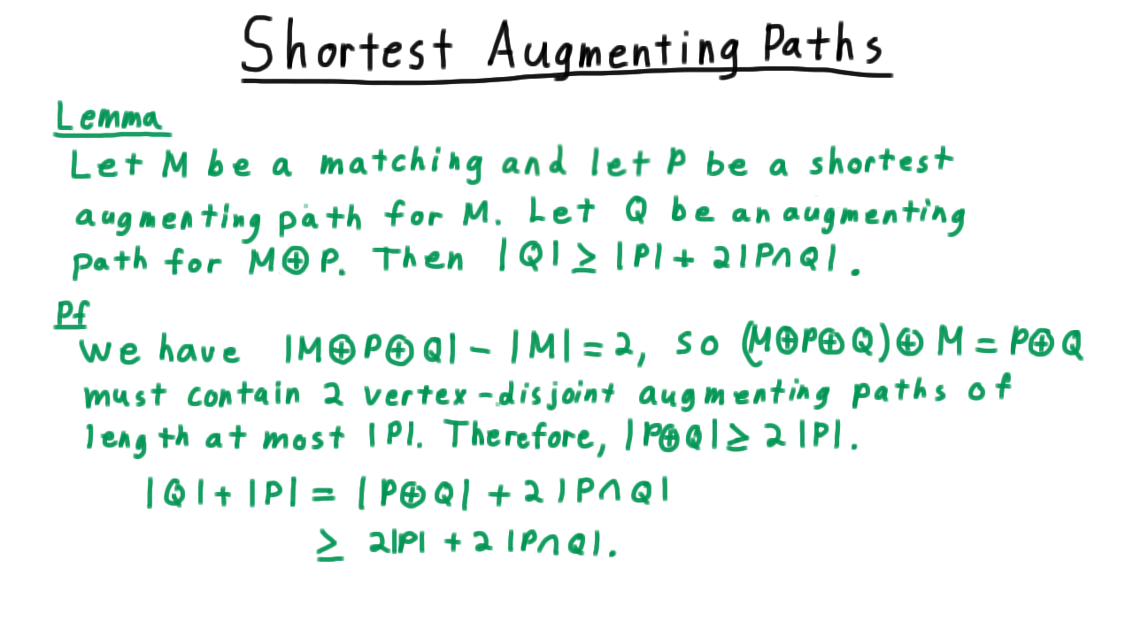
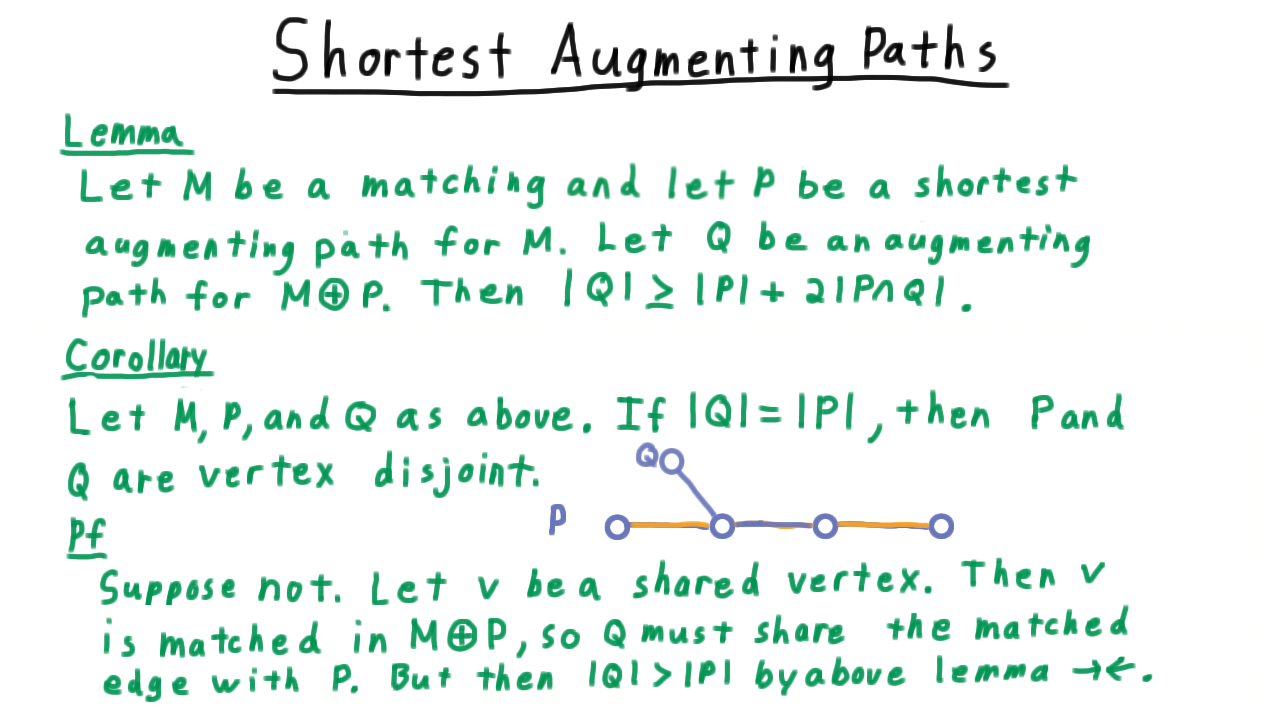
This lemma also has an important corollary.
Analysis of a Phase - (Udacity, Youtube)
Our next lemma states the key property of a phase of the Hopcroft-Karp algorithm.
Each phase increases the length of the shortest augmenting path by at least two.
Let \(Q\) be a shortest augmenting path after phase with path length \(k.\) It’s impossible for \(|Q|\) to be less than \(k\) by a previous lemma, which showed that augmenting by a shortest augmenting path never decreased the minimum augmenting path length.
On the other hand \(|Q|\) being equal to \(k\) implies that Q is vertex disjoint from all paths found in the phase. But then it would have been part of the phase, so this isn’t possible either.
Thus, \(|Q| > k, \) and also odd because it is augmenting, so \(|Q| \geq k + 2,\) completing the lemma.
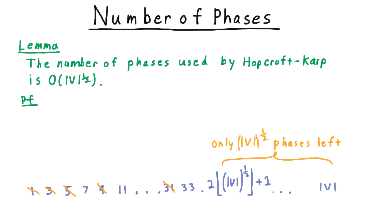
Number of Phases - (Udacity, Youtube)
Now that we know that each phase must increase the length of the shortest augmenting path by at least two, we are ready to bound the number of phases. Specifically, the number of phases used by Hopcroft-Karp is \(O(\sqrt{V}).\) Note that the trivial bound saying that there can be only one phase per possible augmenting path length isn’t good enough. That would still leave us with an \(O(V)\) bound.
In reality, we will have a phase for length 1 and length 3, probably for length 5, maybe not for length 7 and so forth, but as we consider greater lengths the ones for which we will have augmenting phases get sparser and sparser.
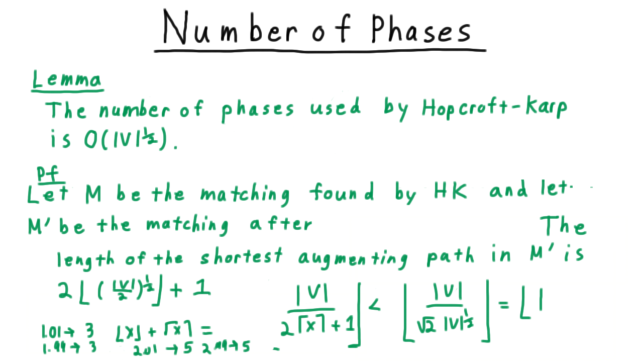
The key argument will be that after roughly \(\sqrt{V}\), there will only be \(\sqrt{V}\) phases left. Let \(M'\) be the matching found by Hopcroft-Karp and let \(M\) be the matching after the \(\lceil \sqrt{V} \rceil\) phases. Because each phase increased the shortest augmenting path length by two, the length of the shortest augmenting path in M is \(2\lceil \sqrt{V} \rceil + 1.\)
Hence, no augmenting path in the difference between \(M'\) and \(M\) can have shorter length. This implies that there are at most \(|V|\) divided by this length augmenting paths in the difference. We just run out of vertices. If there can be only so many augmenting paths in the difference, then M can’t be too far away from \(M'\) – certainly, at most \(\sqrt{V}.\)
Hence M will only be augmented square root of V more times, meaning that there can’t be more than \(\sqrt{V}\) more phases.
We have \(\sqrt{V}\) phases to make all of the augmenting paths long enough so that there can’t only be \(\sqrt{V}\) more possible augmentations. That completes the theorem.
In summary, then the Hopcroft-Karp algorithm yields a maximum bipartite matching in \(O(E\sqrt{V})\) time.
Conclusion - (Udacity, Youtube)
That concludes our lesson on max matchings in bipartite graphs. If the topic of matchings is interesting to you, I suggest exploring matchings in general graphs, instead of just bipartite ones we studied here, and also taking a look at minimum cost matchings and the Hungarian algorithm. Good references abound.