Computability, Complexity, and Algorithms
Charles Brubaker and Lance Fortnow
Computability, Complexity, and Algorithms
Charles Brubaker and Lance Fortnow
Approximation Algorithms - (Udacity)
Introduction - (Udacity, Youtube)
So far in our discussion of algorithms, we have restricted our attention to problems that we can solve in polynomial time. These aren’t the only interesting problems, however. As we saw in our discussion of NP-completeness there are many practical and important problems for which we don’t think there are polynomial algorithms. In some situations, the exponential algorithms we have are good enough, but we can’t obtain any guarantees of polynomial efficiency for these problems, unless P=NP.
Besides resorting to exponential algorithms, we also have the option of approximation. For instance, we might not be able to find the minimum vertex cover in polynomial time, but we can find one that is less than twice as big as it needs to be. And many other NP-complete problems admit efficient approximations as well. This idea of approximation will be the subject of this lesson.
An Approximation for Min Vertex Cover - (Udacity, Youtube)
We’ll start our discussion with a very simple approximation algorithm, one for the minimum vertex cover problem.
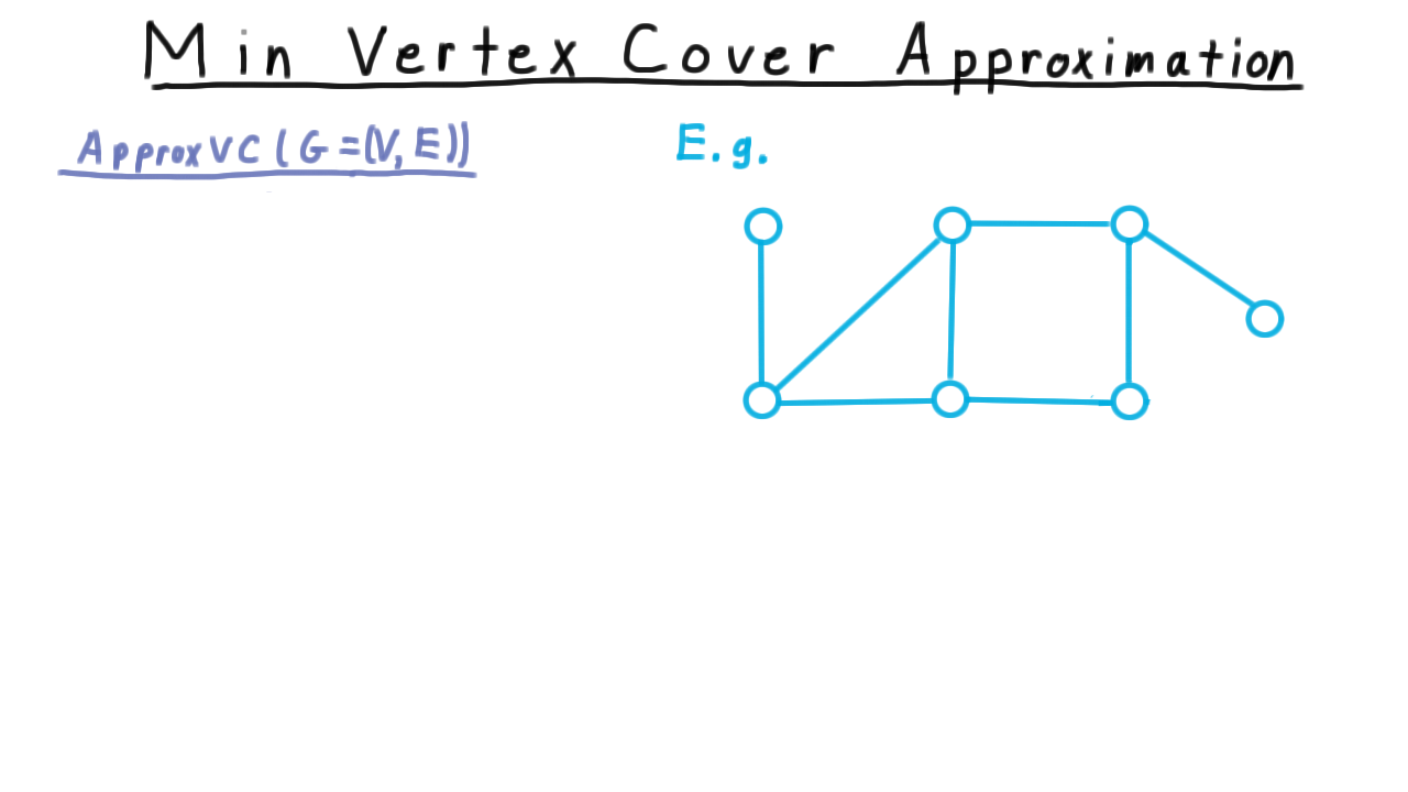
As input, we are given a graph and we want to find the smallest set of vertices such that every edge has at least one end in this set. Recall that this problem is NP-complete. We reduced maximum independent set to it earlier in the course.
The approximation algorithm goes like this.
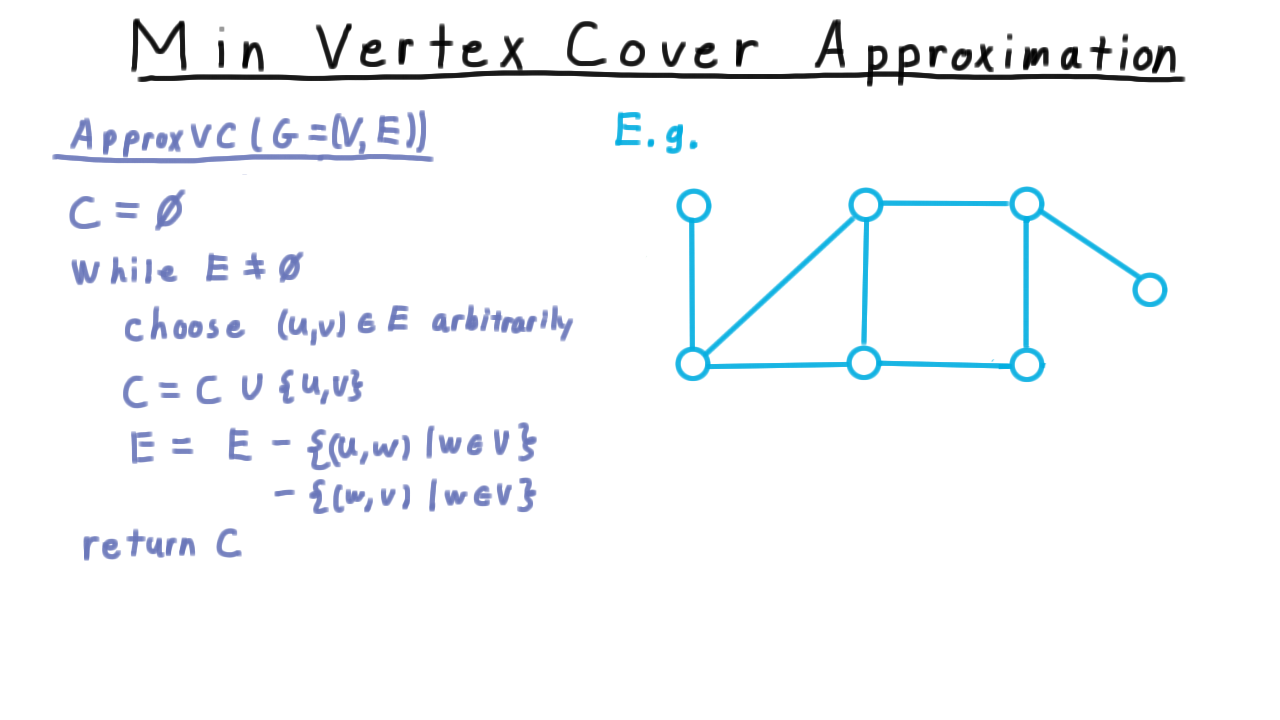
We start with an empty set, and then while there is still an edge that we haven’t covered yet, we chose one of these edges arbitrarily and add both vertices to the set. Then we remove all the edges incident on \(u\) and all those incident on \(v,\) since those edges are now covered. Next, we pick another edge and remove all edges incident on it. And so on, and so forth until there aren’t any edges left. At the end of this process the set C, which we’ve picked must be a cover. (See the video for an animation.)
Looking back at the original graph, it’s not too hard to see that a cover obtained in this way need not be a minimum one. Here is a cover obtained with the algorithm (orange) and optimal cover (green).

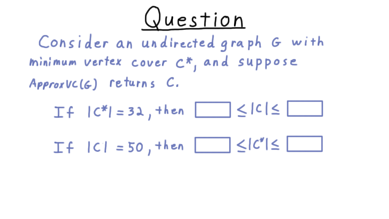
In this case, ApproxVC algorithm returned a cover twice as large as the optimal cover. Fortunately, this is as bad as it gets.
Given a graph \(G\) that has minimum vertex cover \(C^*\), the algorithm VCApprox returns a vertex cover \(C\) such that \(\frac{|C|}{|C^*|} \leq 2.\)
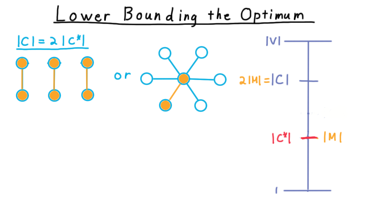
To prove this, it is useful to consider the set of edges chosen by the algorithm at the start of an iteration. We’ll call this set \(M.\) We use the letter \(M\) here because this set is a maximal matching. It pairs off vertices in such a way that no vertex is part of more than one pair. In other words, this set of edges must be vertex disjoint. That means that in order to cover just this set of edges, any vertex cover must include at least one vertex from each. Therefore, \(|M| \leq |C^*|.\)
Since \(C*\) is a minimum cover, the set \(C\) chosen by the algorithm can only be larger. It is of size \(2|M|\). Altogether then,
\[ |M| \leq |C^*| \leq |C| = 2|M| \leq 2|C^*|. \]
Dividing through by \(|C^*|\) then gives the desired result.
\(C\) and \(C^*\) - (Udacity)
Given this theorem, let’s explore the relationship between the size of the optimum cover and the one returned by our ApproxVC algorithm with a quick question. Suppose that \(G\) is a graph with a minimum vertex cover \(C^*\) and that our ApproxVC algorithm returned a set of vertices \(C.\) Fill in these blanks below so as to make these statements as strong as possible.
Lower Bounding the Optimum - (Udacity, Youtube)
Even though the algorithm we just discussed for minimum vertex cover was very simple, it illustrates some key ideas found in many approximation schemes.
Consider this figure here, illustrating the possible sizes of the minimum set cover.
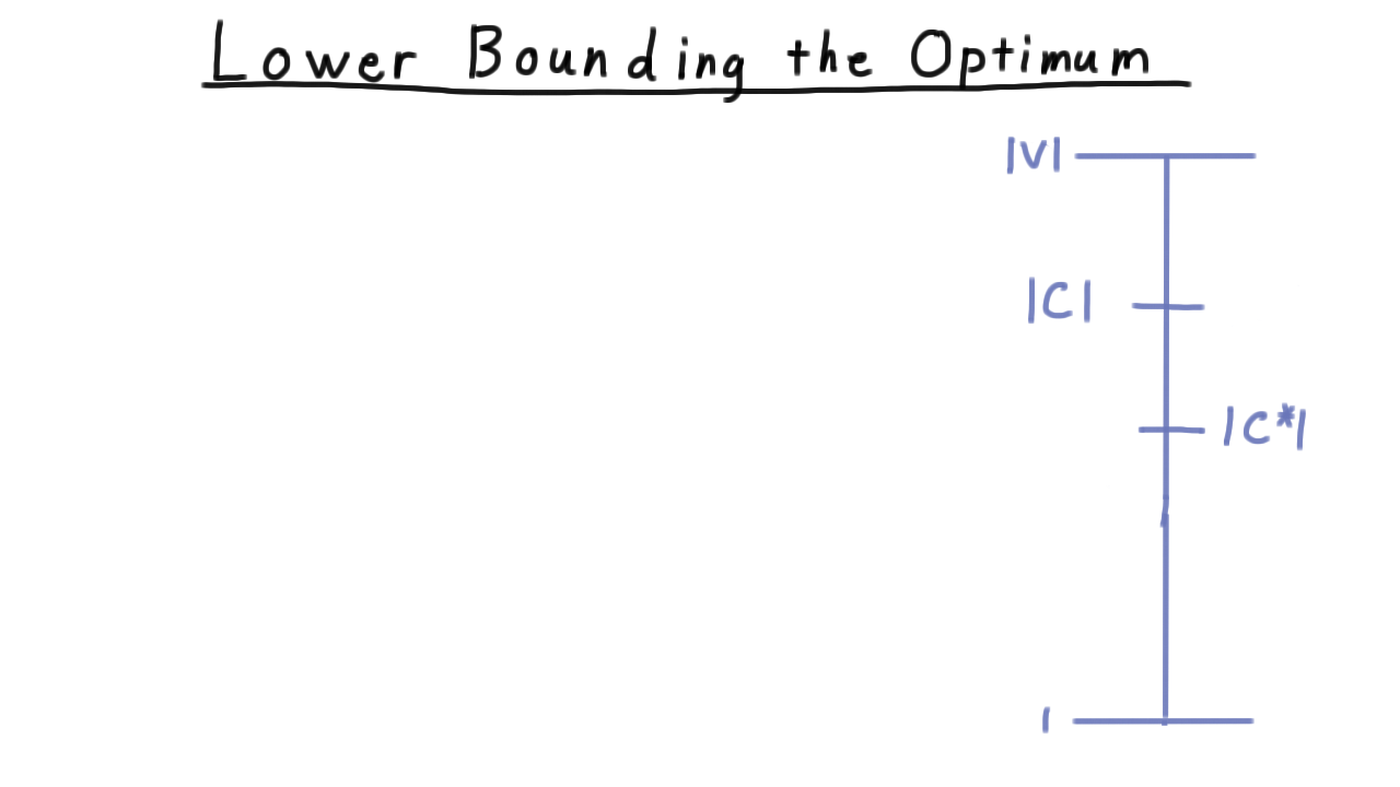
We have the size of the set returned by our algorithm \(|C|\) and size of the optimal one \(C^*.\) We would like to be able to find some GUARANTEE about the relationship between the two. The trouble, of course, is that we don’t know the optimal value. Actually, finding the optimal value is NP-complete, and that’s why we are searching for an approximation algorithm anyway.
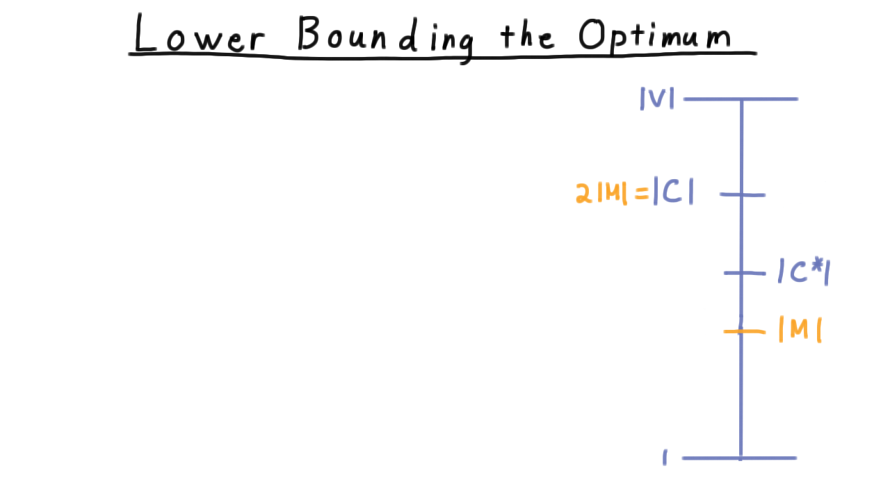
We resolve this dilemma by finding a lower bound on the size of the optimal cover in the maximal matching that the algorithm finds. Then we find the UPPER bound on our approximation then in terms of this lower bound. Note that the approximation is not enough to tell us enough about optimum value to allow us to solve the decision version of the problem: does the graph have a vertex cover of a particular size?
Our approximation might be twice the optimum value,
or it might find an exact solution

Since we can’t tell which situation we are in, we can’t tell where in this range the the minimum vertex cover falls.
Optimization - (Udacity, Youtube)
In our discussion of computability and complexity, we focused on deciding languages. As we began our discussion of algorithms, however, we began to talk about optimization problems instead without ever formally defining them. This was fine then, but as we discuss approximation algorithms, we are going to circle back to some of the ideas we encountered in complexity and we need a formal way to connect them.
Therefore, we are going to define an optimization problem, using min vertex cover as an example to illustrate, and this will allow us to give a formal definition of an approximation algorithm.
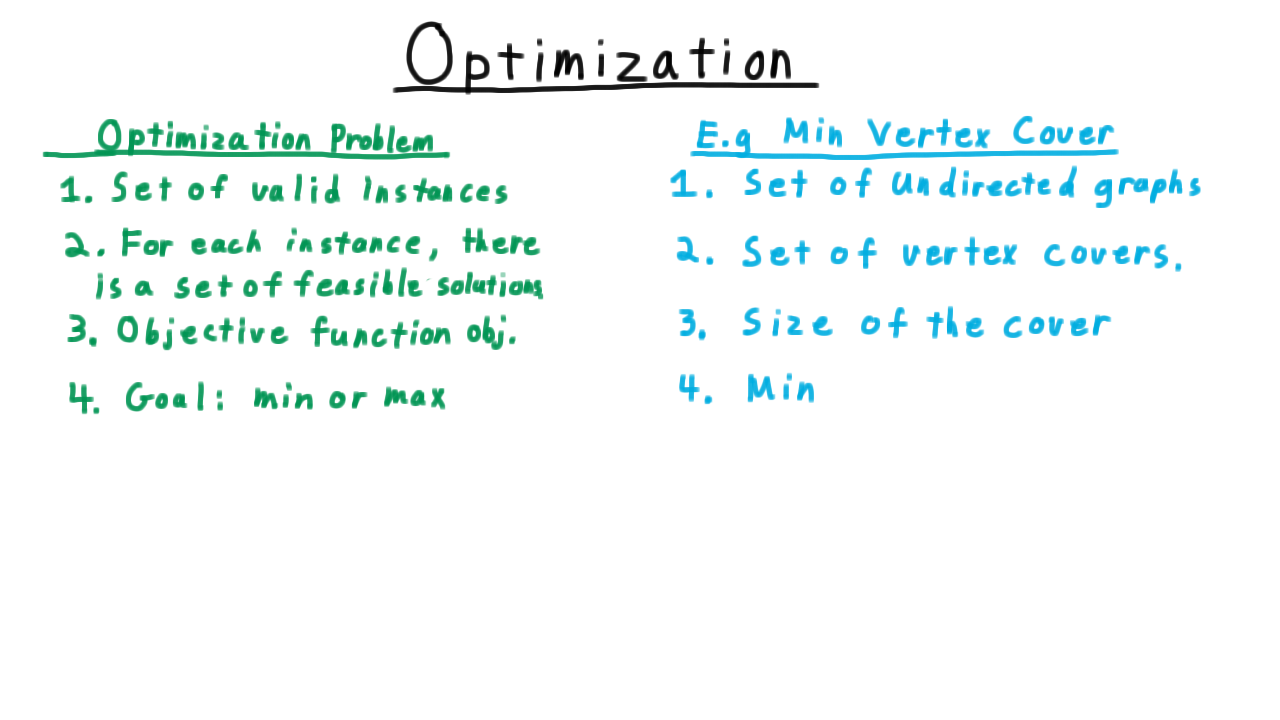
The first thing we need is a set of problem instances. For the example of minimum vertex cover this is just the set of undirected graphs. For each instance, there is a set of feasible solutions. For min vertex cover, this is the set of covers for the graph. Next, we need an objective function, the thing we are trying to optimize. For min vertex cover this is the size of the cover. And we need to say whether we are minimizing or maximizing the objective. For min vertex cover, we are minimizing it of course.
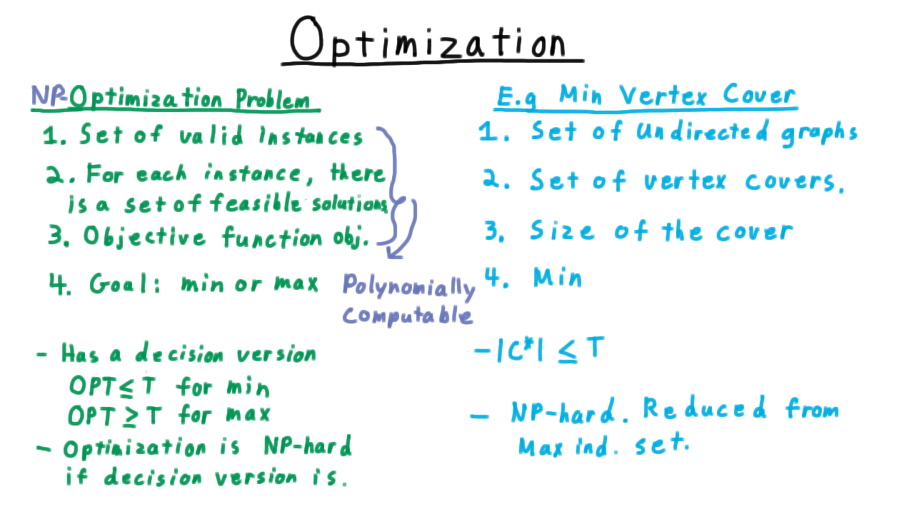
Relating this back to our treatment of complexity, we say that an NP-optimization problem is one where these first three criteria are computable in polynomial time. That is to say, there is a polynomial algorithm that says whether the input instance is value, one that can check whether a solution is feasible for the given instance, and one that can evaluate the objective function.
Now, every optimization problem has a decision version of the form, is the optimum value at most some value for the min and at least some value for the max. For minimum vertex cover, we ask is there a cover of size less than some threshold. With this in mind, we can then say an optimization problem is NP-hard if it’s decision version is. A problem is NP-hard, by the way, if an NP-complete problem can be reduced to it. In our example, min vertex cover is NP-hard because the decision version is. Remember that reduced from the maximum independent set problem.
So that’s how optimization relates to complexity.
Approximation Algorithms - (Udacity, Youtube)
Next, I want to use these definitions of an optimization problem to define an approximation algorithm.
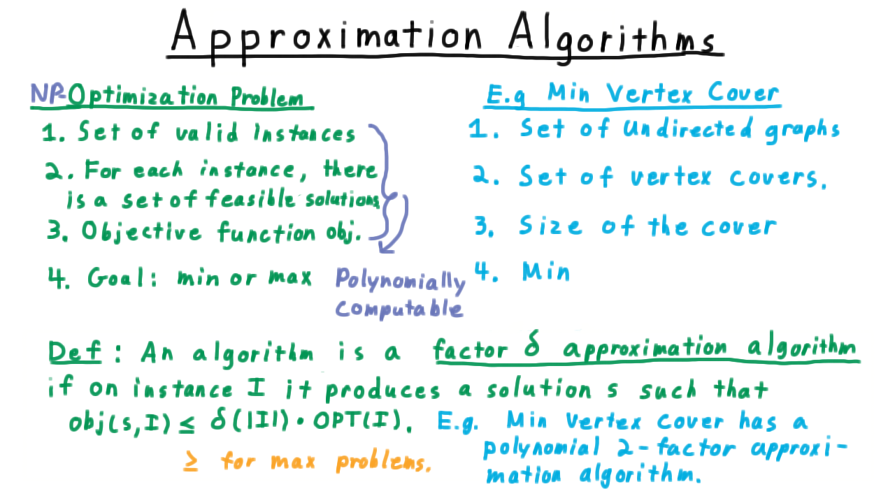
Note that it’s okay for \(\delta\) to be a function of the instance size.
Also, when we are working with maximization problems instead of minimization ones, this inequality gets reversed. Our previous result for the min vertex cover problem can be stated like in terms of this definition by saying “Min vertex cover has a polynomial factor 2 approximation algorithm or approximation scheme.”
An Approximation for Maximum Independent Set - (Udacity)
As we saw earlier in the course, the complement of a minimum vertex cover is a maximum independent set. It’s natural to ask then, can we turn our 2-factor algorithm for minimum vertex cover into an algorithm for maximum independent set? Such an approach yields what about maximum independent set?
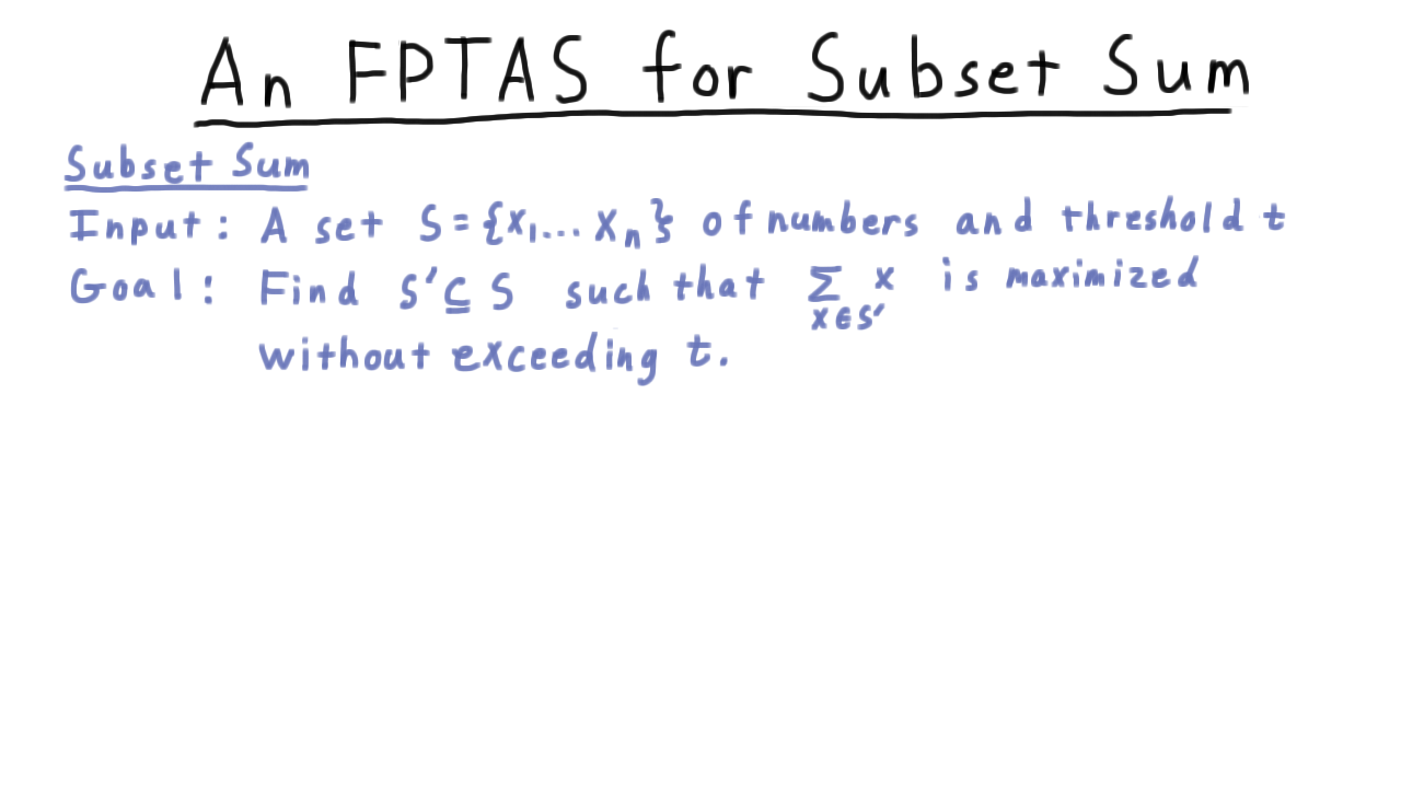
An FPTAS for Subset Sum - (Udacity, Youtube)
The subset sum problem admits a fully polynomial time approximation scheme, or FPTAS for short. Recall that the decision version for subset sum, was whether give a set of numbers there was any subset that summed up to a particular value. The optimization version of this is to maximize the sum without going over some threshold \(t.\)
This problem admits a very important class of approximations.
For any \(\epsilon > 0\), there is an \(O(\frac{n^2 \log t}{\epsilon})\) time, factor \((1+\epsilon)^{-1}\) algorithm for subset sum.
The smaller the epsilon, the better the approximation, but he worse the running time.
This is a remarkable result. It may be intuitive that one should be able to trade-off spending more time for a better approximation guarantee, but it isn’t always the case that we get to do so arbitrarily as in this theorem. Because this isn’t a particular algorithm but rather a kind of recipe for producing an algorithm with the right properties, we call this a polynomial time approximation scheme, or PTAS for short. For every \(\epsilon,\) you choose there is algorithm that can approximate that well.
This approximation scheme is extra special because the running time is polynomial in \(1/\epsilon\) as well as polynomial the size of the input. Therefore, we say that this is a fully polynomial time approximation scheme.The alternative would be for the epsilon to appear in one of the exponents, perhaps. Then it would just be a polynomial time approximation scheme.
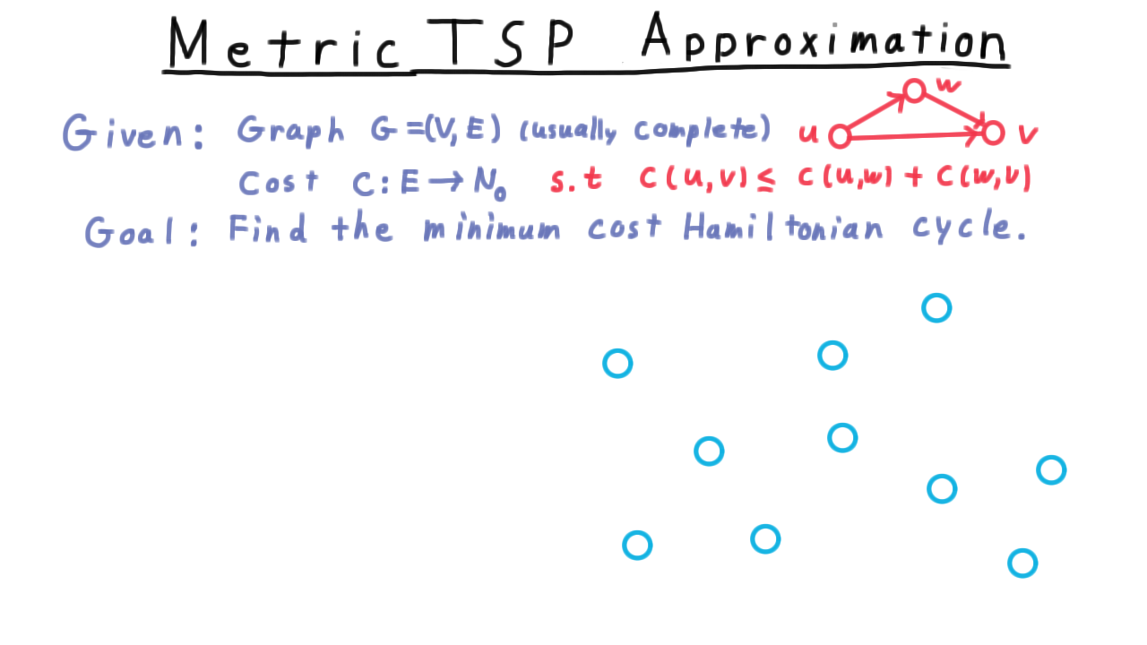
Traveling Salesman Problem - (Udacity, Youtube)
After hearing about these approximation schemes, the optimists may be saying, “hey, maybe every NP-complete problem admits an FPTAS.” Unfortunately, this isn’t true unless P=NP. There are some problems where approximating the optimum within certain factors would lead to a polynomial algorithm for solving every problem in NP. This phenomenon is known as “Hardness of Approximation,” and it occupies an important place in the study of complexity.
We’ll illustrate this idea by showing that the Traveling Salesman Problem is hard to approximate to within any constant factor.
In case you haven’t seen the traveling salesman problem before, it can be stated like this.

We are given a graph G. Usually, all the edges are present, and with each of them is associated some cost or distance. We’ll assume that all the edges are present, so we won’t draw them in our examples like this one here. The goal is to find the minimum cost Hamiltonian cycle. That is to say, we want to visit each of the vertices without ever visiting the same one twice.
This problem is NP-complete in general. And even a constant factor approximation is impossible unless P=NP, as we will prove next.
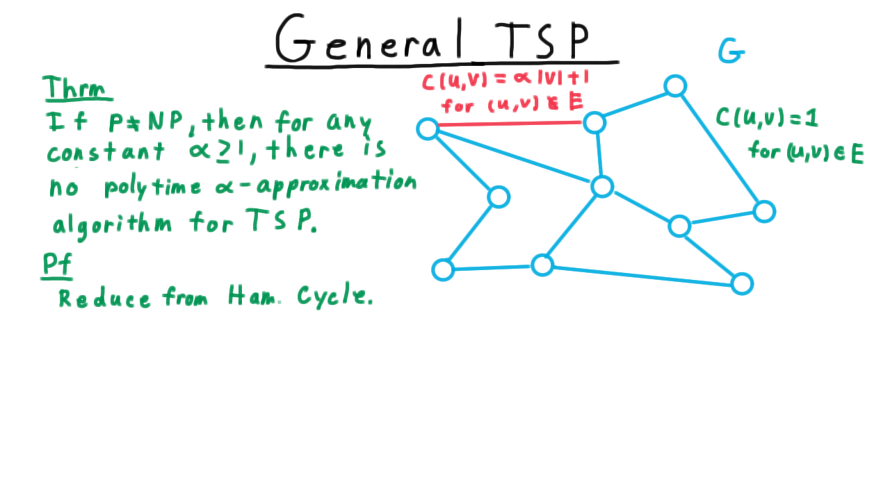
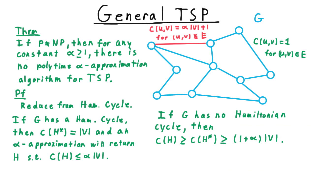
Hardness of Approximation for TSP - (Udacity, Youtube)
Being a little more formal, we can say
If P is not equal to NP, then for any constant \(\alpha \geq 1\), there is no polytime factor \(\alpha\) approximation algorithm for the Traveling Salesman problem.
For the proof, we reduce from the Hamiltonian cycle problem, where are given a graph, not necessarily complete this time, and we want to know if there is a cycle that visits every vertex exactly once. Here then is how we set up the traveling salesman problem. We assign a cost of 1 to every edge in the original graph \(G\) and assign a cost of \(\alpha |V| + 1\) for every edge not in the original graph.
Clearly, then if \(G\) has a Hamiltonian cycle, then the optimum for the traveling salesman problem has a cost of \(|V|\), with a cost of 1 for every edge that it follows. A factor \(\alpha\) approximation would then find a Hamiltonian cycle with cost at most \(\alpha |V|.\) Letting \(H^*\) be an optimal Hamiltonian cycle for the TSP problem and letting \(H\) be the cycle returned by the \(\alpha\)-approximation , we have that
\[ c(H) \leq \alpha |V|.\]
On the other hand, if the original graph \(G\) has no Hamiltonian cycle, then the cost of the one returned by the approximation algorithm must be at least as large as the optimum, which must follow at least one edge not in the original graph. Hence,
\[c(H) \geq c(H^*) \geq |V| - 1 + \alpha|V| + 1. \]
This term on the right hand side comes from the edges in the original graph, and the second from following one of the edges not in the original graph. Simplifying gives the lower bound of \((1 + \alpha)|V|\).
Therefore, to decide Hamiltonian cycle, we just run the \(\alpha\)-approximation on the graph and compare the resulting cost to \(\alpha |V|\). If it is larger, then there can’t be a Hamiltonian cycle in the graph. On the other hand, if the same or smaller, then we can’t have used one of the edges not in the original graph, so there must be a Hamiltonian cycle.
Thus, if there were polynomial constant factor approximation for the Traveling Salesman problem, it would yield a polynomial algorithm for Hamiltonian cycle, which is NP complete. Unless P is equal to NP, no such approximation algorithm can exist.
Summary - (Udacity, Youtube)
So far, we’ve seen three different kinds of results related to approximation algorithms. We seen a factor 2 approximation in the example of Vertex cover. We talked about Fully Polynomial Time Approximation Schemes in the context of subset sum. And we’ve seen a hardness of approximation result in showing that the general traveling salesman problem cannot be approximated to within any constant factor. That’s a good sample of the types of results ones sees in the study of approximation algorithms.
Before ending this lesson, however, I want to talk about one more classic result.
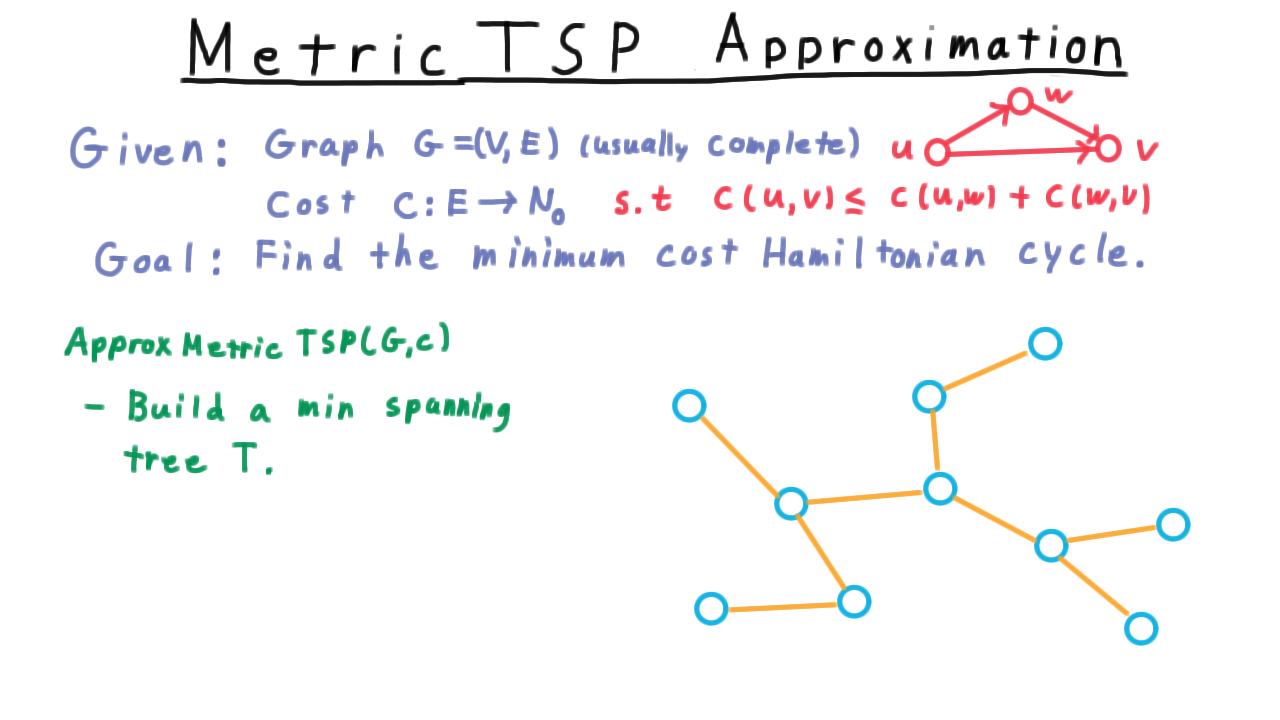
Metric TSP - (Udacity, Youtube)
Perhaps the traveling salesman problem can’t be approximated in general, but if we insist that the cost function obey the triangle inequality as it does in many practical applications, then we can find an approximation. The triangle inequality, by the way, just says that is never faster to go from one vertex to another via a third vertex.
Here is the approximation algorithm. We start by building a minimum spanning tree. The usual approach here is to use one of the greedy algorithms, either of Kruskal or Prim, that are typically taught in an undergraduate class. In Kruskal’s algorithm, the idea is simply to take the cheapest edge between two unconnected vertices and add that the graph until a tree is formed. (See the video for an animation.)
Next, we run a depth-first search on the tree, keeping track of the order in which the vertices are discovered. For this example, let’s label the vertices with the letters of the alphabet, and start from C. Then the discovery order would go something like this.
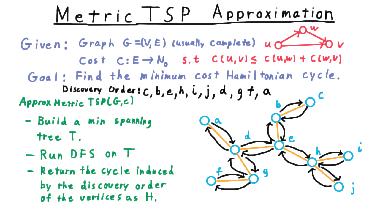
Note that this cycle follows along the tree at first, from c to b to e to h to i, nut instead of back tracking to h, it goes directly to j. Then, it goes directly to d, and so on.
This cycle seems to always be taking short-cuts compared to the traversal the depth-first search performed. For the general Traveling Salesman problem, we can’t be sure these are in-fact short-cuts, because we can’t assume the triangle inequality. Where we do have the triangle inequality, however, these *will be short cuts, and as we’ll see that will be the key to the analysis.
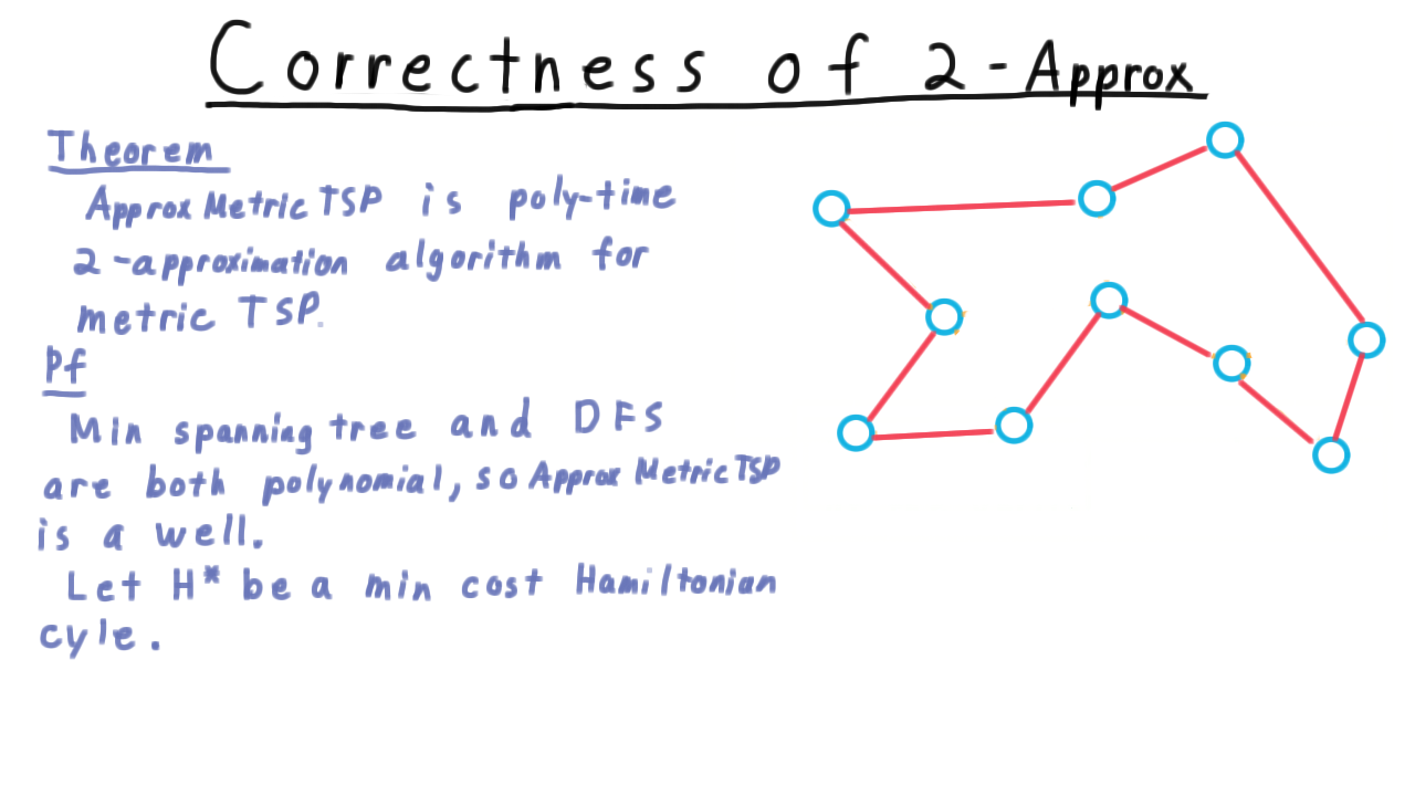
Correctness of Factor 2 TSP Approx - (Udacity, Youtube)
The algorithm just described, which we call ApproxMetricTSP, is an \(O(V^2)\) time, factor 2 approximation algorithm for the metric traveling salesman problem.
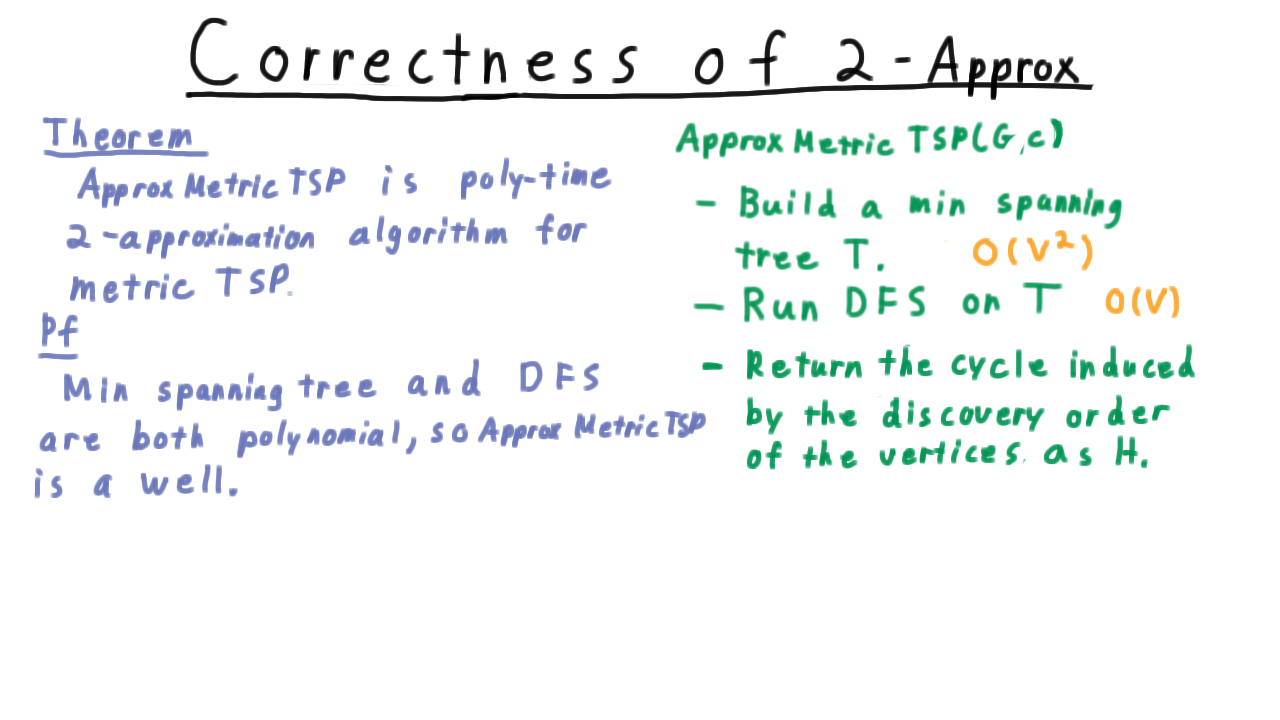
The process for building the min spanning tree is \(O(V^2)\) for dense graphs and the depth first search process takes time proportional to the number of edges, which is the same as being proportional to the number of vertices for trees. That takes care of the efficiency of the algorithm.
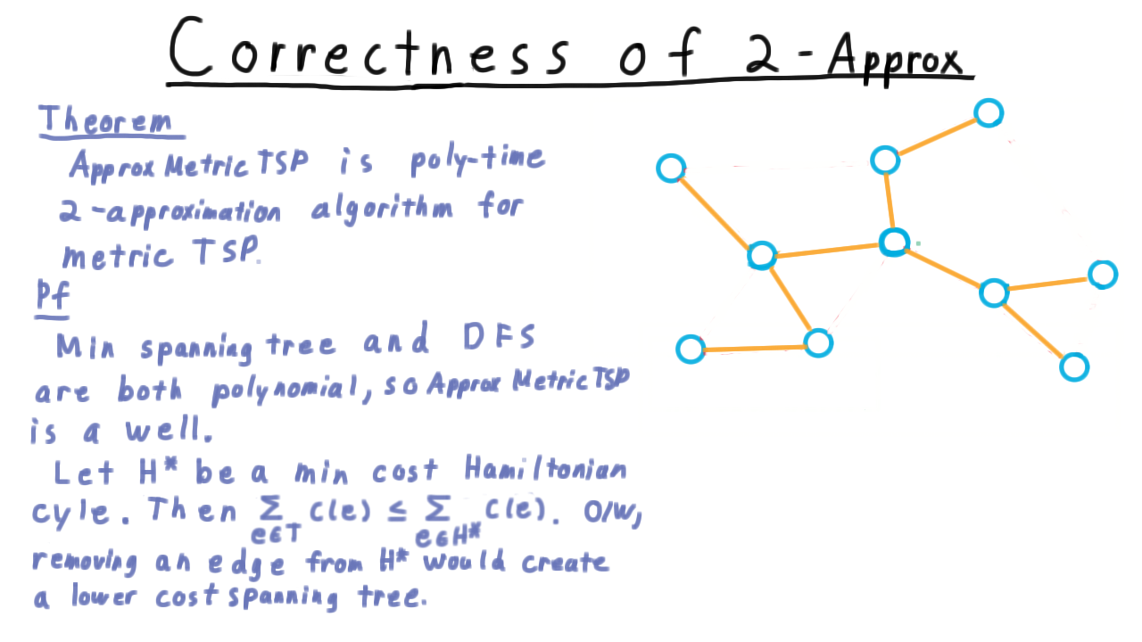
Now for the factor-two part. Consider this example here,
and let \(H^*\) be a minimum cost Hamiltonian cycle over this graph. This is what an exact algorithm might output. Well, the cost of the minimum spanning tree that the algorithm finds must be less than the total cost of the edges in this cycle. Otherwise, just removing an edge from the cycle would create a lower cost minimum spanning tree. (Remember that the cost must be non-negative). Thus, for a minimum spanning tree \(T\), we have
\[\sum_{e\in T} c(e) \leq \sum_{e\in H^*} c(e).\]
Now, let’s draw a minimum cost spanning tree.
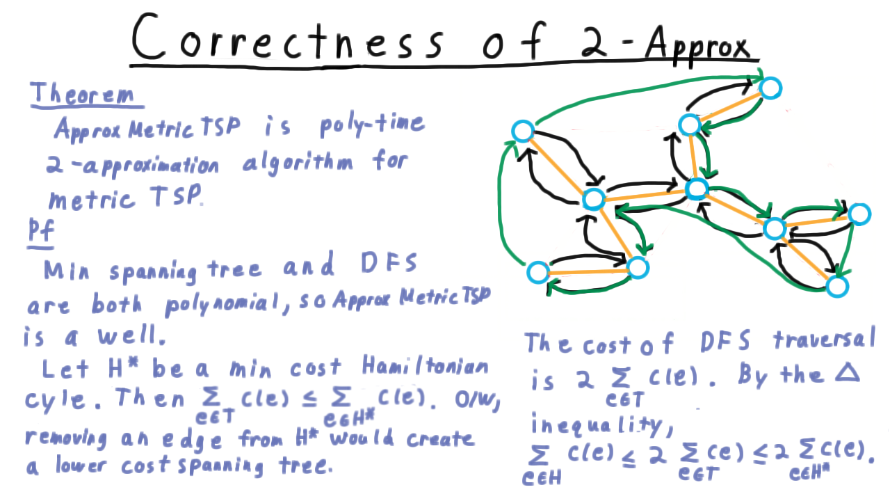
The cost of a depth-first search traversal is twice the sum of the costs of the edges in the tree, i.e. \(2\sum_{e \in T} c(e)\) This also starts and ends at the same vertex, so it’s a cycle.
The trouble is that it’s not Hamiltonian. Some vertices might get visited twice. It’s easy enough, however, to count only the first time that a vertex is visited. In fact, this is what ordering the vertices by their discovery time achieves.
By the triangle inequality, skipping over intermediate vertices can only make the path shorter, so the cost of this cycle is most the cost of the depth-first traversal. Thus,
\[c(H) \leq 2\sum_{e \in T} c(e) \leq 2 \sum_{e \in H^*} c(e) = 2c(H^*).\]
That’s the proof of the theorem.
It may also be useful to view the argument on a scale like this one with 0 at the bottom, maybe the cost of the most expensive cycle at the top and the optimal one somewhere in the middle.
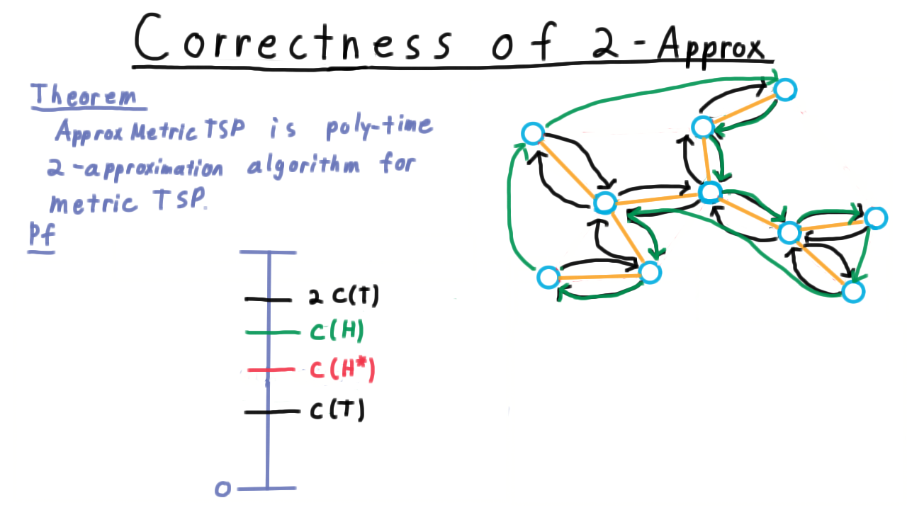
As we argued, the cost of a minimum spanning tree must be less than the cost of the optimum cycle. We can just delete one edges from the cycle and get a spanning tree. A depth first traversal of the spanning tree uses every edge twice, and therefore is twice the cost of the tree. Shortcutting all but the first visit to a vertex in this traversal gives a Hamiltonian cycle, which MUST have lower cost because of the triangle inequality.
A Tight Example Part 1 - (Udacity)
In response to any approximation result, it is natural to ask, “is the analysis tight or does the algorithm actually perform better even in the worst case than the theorem says.” Let’s address that question for our metric TSP algorithm.
Here is an example graph.
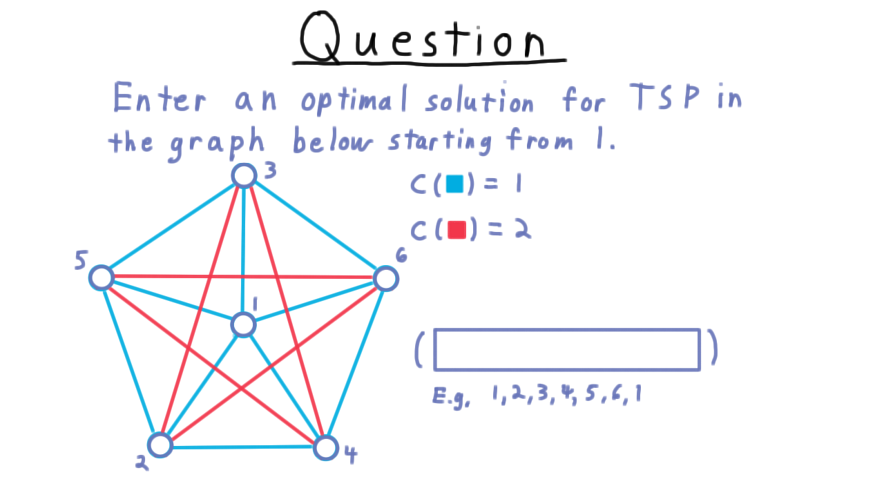
Let the blue edges have cost 1 and the red ones have cost 2. Enter a minimum cost solution in the box below.
A Tight Example Part 2 - (Udacity)
Now, we consider what our approximation algorithm might have returned. Recall that the optimum is a Hamiltonian cycle of cost 6. The approximation algorithm begins by building a minimum spanning tree for the graph. Perhaps, it chooses the star, like so.
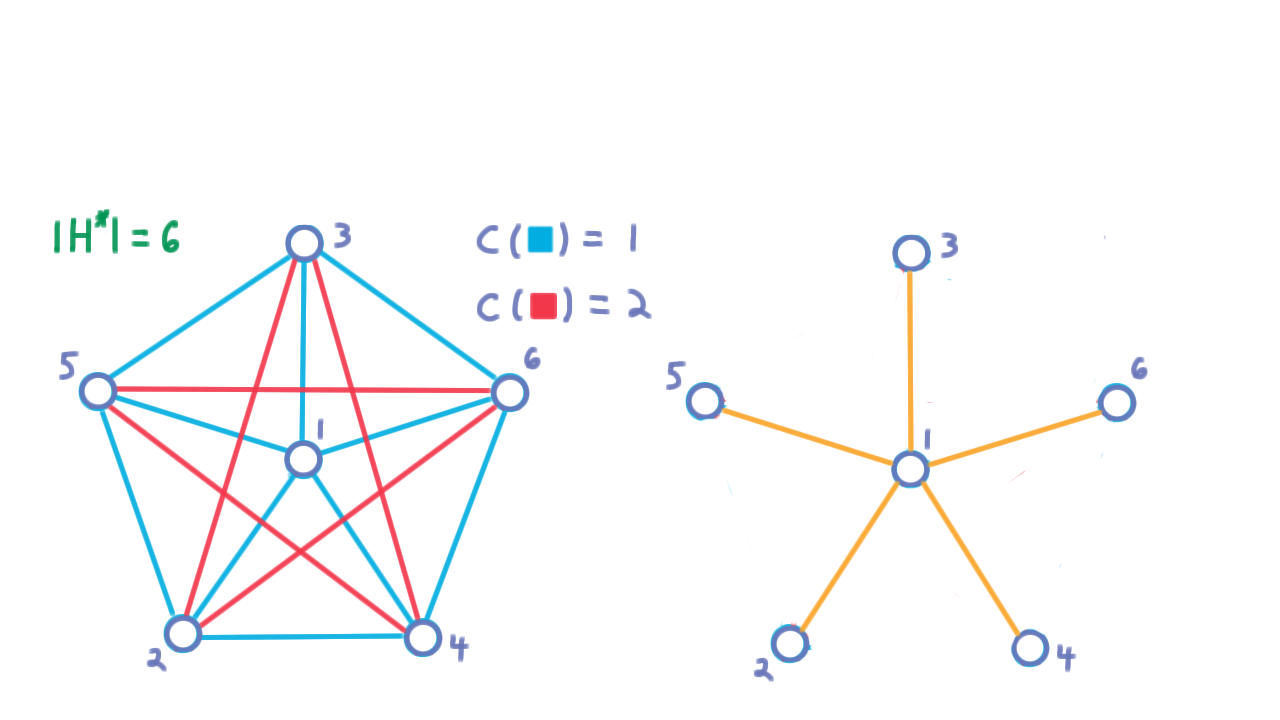
Then, preferring lowest indexed vertices a depth-first traversal would produce this cycle.
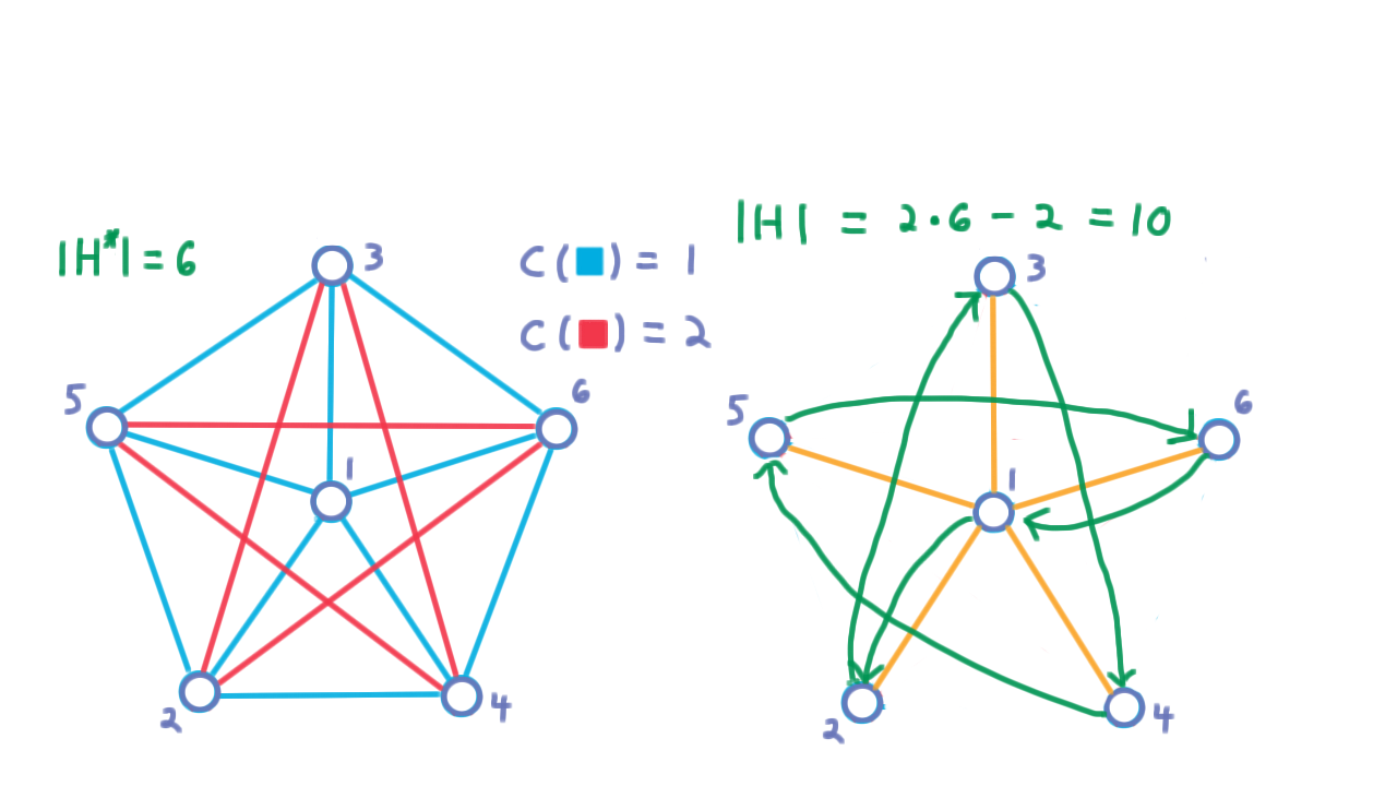
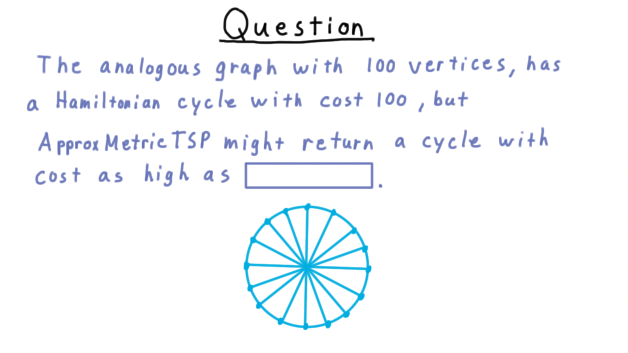
Notice that every edge followed in this cycle is a red one except the first and the last. Hence the cost is \(2 \cdot 6 - 2 = 10.\) The ratio is therefore \(10/6\). But there wasn’t really anything special about the fact that we were using \(6\) vertices here. We can form an analogous graph for any \(n,\) letting the lighter edges be the union of a star and a cycle around the non-center vertices. All other edges can be heavy.
My question to you then is how bad does the approximation get for \(100\) vertices? Give your answer in this box.
Conclusion - (Udacity, Youtube)
In this lesson, we’ve just scratched the surface of the vast literature on approximation algorithms. One could create a whole course on the subject consisting just of results not much more complicated than the ones we’ve seen here. And, of course, there are many more advanced results besides. The main take-away message then is that when you encounter a problem where finding an optimum solution seems intractable, ask yourself, “is an approximate solution good enough?” You may find that relaxing the optimality constraint makes the problem tractable.