Formal Languages - Udacity
Functions and Computable Functions - (Udacity,Youtube )
In school, it is common to develop a certain mental conception of a function. This conception is often of the form:
A function is a procedure you do to an input (often called x) in order to find an output (often called f(x)).
However, this notion of a function is much different from the mathematical definition of a function:
A function is a set of ordered pairs such that the first element of each pair is from a set X (called the domain), the second element of each pair is from a set Y (called the codomain or range), and each element of the domain is paired with exactly one element of the range.

The first conception—the one many of us develop in school—is that of a function as an algorithm: a finite number of steps to produce an output from an input, while the second conception—the mathematical definition—is described in the abstract language of set theory. For many practical purposes, the two definitions coincide. However, they are quite different: not every function can be described as an algorithm, since not every function can be computed in a finite number of steps on every input. In other words, there are functions that computers cannot compute.
Rules of the Game - (Udacity, Youtube)
When you hear the word computation, the image that should come to mind is a machine taking some input, performing a sequences of operations, and after some time (hopefully) giving some output.

In this lesson, we will focus on the forms of the inputs and output and leave the definition of the machine for later.
The inputs read by the machine must be in the form of strings of characters from some finite set, called the machine’s alphabet. For example, the machine’s alphabet might be binary (0s and 1s), it might be based on the genetic code (with symbols A, C, G, T), or it might be the ASCII character set.
Any finite sequence of symbols is called a string. Thus, ‘0110’ is a string over the binary alphabet. Strings are the only input data type that we allow in our model.
Sometimes, we will talk about machines having string outputs just like the inputs, but more often than not, the output will just be binary–an up or down decision about some property of the input. You might imagine the machine just turning on one of two lights, one for accept, or one for reject, once the machine is finished computing.

With these rules, an important type becomes a collection of strings. Maybe, it’s the set of strings that some particular machine accepts, or maybe we are trying to design a machine so that it accepts strings in a certain set and no others, or maybe we’re asking if it’s even possible to design a machine that accepts everything in some particular set and no others. In all these cases, it’s a set of strings that we are talking about, so it makes sense to give this type its own name.
We call a set of strings a language. For example, a language could be a list of names, It could be the set of binary strings that represent even numbers–notice that this set is infinite–or it could be the empty set. Any set of strings over an alphabet is a language.
Operations on Languages - (Udacity, Youtube)
The concept of a language is fundamental to this course, so we’ll take a moment to describe common operations used to manipulate languages. For examples we’ll use the languages \(A = \){’0‘,10’} and \(B = \) {’0’,‘11’} over the zero-one alphabet.
Since languages are sets, we have the usual operations of union, intersection and complement defined for them. For example \(A\) union \(B\) consists of the three strings ‘0’,‘10’, and ‘11’. The string ‘0’ comes from both \(A\) and \(B\), ‘10’ from \(A\) and ‘11’ from \(B\). The intersection contains only those strings in both languages, just the string ‘0’.
To define the complement of a language we need to make clear what it is that we are completing. It’s not sufficient just to say that it is everything not in \(A\). For \(A\) that would include strings with characters besides 0 and 1 or maybe even infinite sequences of 0’s and 1’s, which we don’t want. The complement, therefore, is defined so as to complete the set of all strings over the relevant alphabet, in this case the binary alphabet. The alphabet over which the language is defined is almost always clear from context. In this case, the complement of \(A\) will be infinite.

In addition to these standard set operations, we also define an operation for concatenating two languages. The concatenation of \(A\) and \(B\) is just all strings you can form by taking a string from \(A\) and appending a string from \(B\) to it. In our examples, this set would be ‘00’ with first 0 coming from \(A\) and second from \(B\). The string ‘011’ with the ‘0’ coming from \(A\) and the ‘11’ coming from \(B\), and so forth. Of course, we can also concatentate a language with itself. Instead of writing \(AA\), we often write \(A^2\). In general, when we want to concatenate a language with itself k times we write \(A\) to the kth power. Note that for \(k=0\), this defined as the language containing exactly the empty string.
When we want to concatenate any number of strings from a language together to form a new language, we use an operator known as Kleene star. This can be thought of as the union of all possible powers of the language. When we want to exclude the emptry string, we use the plus operator, which insists that at least one string from A be used. Notice the difference in starting indices. So for example, the string ‘01001010’ is in \( A^*\). There is a way that I can break it up so that each part is in the language \(A\), and so as a whole the string can be thought of a concatenation of strings from \(A\). Note that even \(A^*\) doesn’t include infinite sequences of symbols. Each individual string from A must be of finite length, and you are only allowed to concatenate a finite number together.
For those who have studied regular expressions, this should seem quite familiar. In fact, one gets the notation of regular expressions by treating individual symbols a languages. For example, \(0^*\) is the set of all strings consisting entirely of zeros. Here we are treating the symbol 0 as a language unto itself. We will also commonly refer to \(\Sigma^*\), meaning all possible strings over the alphabet \(\Sigma\). Here we are treating the individual symbols of the alphabet as strings in the language \(\Sigma\).
Language Operations Exercise - (Udacity)
Countability (Part 1) - (Udacity, Youtube)
We need one more piece of mathematical background before we can more formally prove our claim that not all functions are computable. Intuitively, the proof will show that there are more languages than there are possible machines. The set of possible computer programs is countably infinite, but the set of languages over an alphabet in uncountably infinite.
If you aren’t familiar with the distinction between countable and uncountable sets already, you may be thinking to yourself “inifinity is a strange enough idea by itself; now I have to deal with two of them!” Well, it isn’t as bad as all that. A countably infinite set is one that you can enumerate–that is, you can say this is the first element, this is the second element, and so forth, and –this is the really important part– eventually give a number to every element of the set. For some sets an enumeration straightforward. Take the even numbers. We can say that 2 is the first one, 4 the second, 6 the third and so forth. For some sets, like the rationals you have to be a little clever to find an enumeration. We’ll see the trick for enumerating them in a little bit. And for some sets, like the real numbers, it doesn’t matter how clever you are; there simply is no enumeration. These are the uncountable sets.
Let us make the following definition:
A set S is countable if it is finite or if it is in one-to-one correspondence with the natural numbers.
A one-to-one correspondence, by the way is a function that is one-to-one, meaning that no two elements of the domain get mapped to the same element of the range, and also onto, meaning the every element of the range is mapped to by an element of the domain. For example, here is a one-to-one correspondence between the integers 1 through 6 and the set of permutations of three elements.

Now, in general, the existence of a one-to-one correspondence implies that the two sets have the same size– that is, the same number of elements. And this actually holds even for infinite sets. This is why we say that there are as many even natural numbers as there are natural numbers: because it’s easy to establish a one-to-one correspondense between the two sets, f(n) = 2n for example. Some examples of countably infinite sets are:
- The set of nonnegative even numbers (a one-to-one correspondence to the natural numbers is \(f(x) = x/2)\)
- The set of positive odd numbers (with correspondence \(f(x) = (x-1)/2\)
- The set of all integers (with correspondence \(f(x) = 2x\) if \(x\) is nonnegative and \(f(x) = -2x - 1\) if \(x\) is negative)
For our purposes, we want to show that the set of all strings over a finite alphabet is countable. Since computer programs are always represented as finite strings, this will tell us that the set of computer programs is countable. The proof is relatively straightforward. Recall that \(\Sigma*\) is the union of strings of size 0 with those of size 1 with those of size 2, etc. Our strategy will just be to assign the first number to \(\Sigma^0\), the next numbers \(\Sigma^1\), the next to \(\Sigma^2\), etc. Here is the enumeration for the binary alphabet.
The key is that every string gets a positive integer mapped to it under this scheme. Therefore,
The set of all strings over any alphabet is countable.
Countability (Part 2) - (Udacity, Youtube)
This same argument shows that
A countable union of finite sets is countable.
Suppose that our set of sets is \(S_0, S_1,…\) etc. Without loss of generality, we’ll suppose that they are disjoint. (If they happen not to be disjoint, we can always make them so by subtracting out from \(S_k\) all the elements it shares with sets \(S_0...S_k-1\).)
Then the argument proceeds just as before. We assign the first numbers to \(S_0\), the next to \(S_1\), etc. Every element in the union must have a first set \(S_k\) that it belongs to, and thus it will be counted in the enumeration.

It turns out that we can actually prove something even stronger than this statement here.
We can replace this word finite with the word countable, and say that
A countable union of countable sets is countable.
Notice that our current proof doesn’t work. If we tried to count all of the elements of \(S_0\) before any of the elements of \(S_1\), we might never get to the elements of \(S_1\), or any other set besides \(S_0\). Nevertheless, this theorem is true. For convenience of notation, we let the elements of \(S_k\) be \(\{x\_{k0}, x\_{k1},…\}\) and then we can make each set \(S_k\) a row in a grid.

Again, we can’t enumerate row-by-row here because we would never finish the first row. On the other hand, can go diagonal-by-diagonal, since each diagonal is finite. The union of all the set S_k is the union of all the rows, but that is the same as the union of all the diagonals. Each diagonal being finite, we can then apply the original version of the theorem to prove that a countable union of countable sets is countable.
Note that his idea proves that the rationals are countable. Imagine putting all fractions with a 1 in the numerator in the first row, all those with a 2 in the numerator in the second row, etc.
A False Proof - (Udacity)

Languages are Uncountable - (Udacity, Youtube)
So far, we’ve seen that the set of strings over an alphabet in countable. But what about all subsets of these strings? What about the set of all languages. It turns out that this set is uncountable.
The set of all languages over an alphabet is uncountable.
For the proof, we’ll suppose not. That is, suppose there is an enumeration of the languages \(L_1, L_2, \ldots \) over an alphabet \(\Sigma\). Also, let \(x_1, x_2,\ldots \) be the strings in \(\Sigma^*\). We are then going to build a table, where the columns correspond to the strings from Sigma* and the rows correspond to the languages. In each entry in the table, we’ll put a 1 if the string is in the language and a 0 if it is not.

Now, we are going to consider a very sneaky language defined as follows: it consists of the those strings \(x_i\) for which \(x_i\) is not in the language \(L_i\). In effect, we’ve taken the diagonal in this table and just reversed it. Since we are assuming that the set of languages is countable, this language must be \(L_k\) for some \(k\). But is \(x_k\) in \(L_k\) or not? From the table, the row \(L_k such\) that in every column the entry is the opposite of what is on the diagonal. But the diagonal entry can’t be the opposite of itself.
If \(x_k\) is in \(L_k\), then according to the definition of \(L_k\), it should not be in \(L_k\). On the other hand, if \(x_k\) is not in \(L_k\), then it should be in \(L_k\). Another way to think about this argument is to say that this oppositie-of-the-diagonal language must be different from every row in the table because it is different from the diagonal element. In any case, we have a contradiction and can conclude that this enumeration of the languages was invalid since the rest of our reasoning was sound. This argument here is known as the diagonalization trick, and we’ll see it come up again later, when we discuss Undecidability.
Consequences - (Udacity, Youtube)
Although they may not be immediately apparent, the consequences of the uncountability of languages are rather profound.
We’ll let \(\Sigma\) be the set of ASCII characters–these are all the ones you would need to program–
and observe that the set of strings that represent valid python programs is a subset of \(\Sigma^*\). Each program is a finite string, after all. (The choice of python arbitrarily– any language or set of languages works.) Since this set is subset of the countable set \(\Sigma^*\), we have it is countable. Thus, there are a countable number of python programs.
On the other hand, consider this fact. For any language \(L\), we can define \(F_L\) to be the function that is 1 if x is in \(L\) and 0 otherwise. All such functions are distinct, so the set of these functions must be uncountable, just like the set of all languages.
Here is the profound point, since the set of valid python programs is countable but the set of functions is not, it follows that there must be some functions that we just can’t write programs for. In fact, there are uncountably many of them!
So going back to our picture of the HS classroom, we can see that the teacher, perhaps without realizing it was talking about something much more general that what the student ended up thinking. There are only countably many computer programs that can follow a finite number of steps as the student was thinking, but there are uncountably many functions that fit the teachers definition.
Computability and Algorithms - Course Notes
Turing Machines - (Udacity)
Motivation - (Udacity, Youtube)
In the last lesson we talked informally about what it means to be computable. But what even is a computer? What kinds of problem can we solve on a computer? What problem can’t be solved?
To answer these questions we need a model of computation. There are many, many ways we could define the notion of computability–ideally something simple and easy to describe, yet powerful enough so this model can capture everything any computer can do, now or in the future.
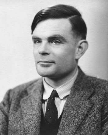
Luckily one of the very first mathematical model of a computer serves us quite well, a model developed by Alan Turing in the 1930’s. Decades before we had digital computers, Turing developed a simple model to capture the thinking process of a mathematician. This model, which we now call the Turing machine, is an extremely simple device and yet completely captures our notion of computability.
In this lesson we’ll define the Turing machine, what it means for the machine to compute and either accept or reject a given input. In future lessons we’ll use this model to give specific problems that we cannot solve.
Introduction - (Udacity, Youtube)
In the last lesson, we began to define what computation is with the goal of eventually being precise about what it can and cannot do. We said that the input to any computation can be expressed as a string, and we assumed that, whatever instructions there were for turning the input into output, that these too could be expressed as a string. Using a counting argument, we were able to show that there were some functions that were not computable.
In this lesson, we are going to look at how input gets turned into output more closely. Specifically, we are going to study the Turing machine, the classical model for computation. As we’ll see in a later lesson, Turing machines can do everything that we consider as computation, and because of their simplicity, they are a terrific tool for studying computation and its limitations. Massively parallel machines, quantum computers they can’t do anything that a Turing machine can’t also do.
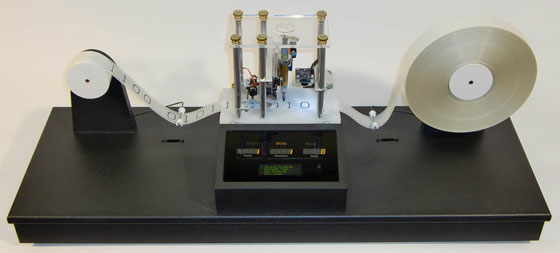
Turing machines were never intended to be practical, but nevertheless several have been built for illustrative purposes, including this one from Mike Davey.
The input to the machine is a tape onto which the string input has been written. Using a read/write head the machine turns input into output through a series of steps. At each step, a decision is made about whether and what to write to the tape and whether to move it right or left. This decision is based on exactly two things:
- the current symbol under the read-write head, and
- something called the machines state, which also gets updated as the symbol is written.
That’s it. The machine stops when it reaches one of two halting states named accept and reject. Usually, we are interested in which of these two states the machine halts in, though when we want to compute functions from strings to strings then we pay attention to the tape contents instead.
It’s a very interesting historical note that in Alan Turing’s 1936 paper in which he first proposed this model, the inspiration does not seem to come from any thought of a electromechanical devise but rather from the experience of doing computations on paper. In section 9, he starts from the idea of a person who he call the computer working with pen and paper, and then argues that his proposed machine can do what this person does.
Let’s follow his logic by considering my computing a very simple number: Alan Turing’s age when he wrote the paper.
\[1936 - 1912 = 24.\]
Turing argues that any calculuation like this can be done on a grid.
Like a child arithmetic book, he says. By this he means something like wide-ruled graph paper. He argues that all symbols can be made to fit inside of one of these squares.
Then he argues, that the fact that the grid is two-dimensional is just a convenience, so he takes away the paper and says that computation can done on tape consisting of a one-dimensional sequence of squares. This isn’t convenient for me, but it doesn’t limit what the computation I can do.
Then points out that there are limits to the width of human perception. Imagine I am reading in a very long mathematical paper, where the phrase “hence by theorem this big number we have …” is used. When I look back, I probably wouldn’t be sure at a glance that I had found the theorem number. I would have to check, maybe four digits at a time, crossing off the ones that I had matched so as to not lose my place. Eventually, I will have matched them all and can re-read the theorem.

Since Turing was going for the simplest machine possible, he takes this idea to the extreme and only let’s me read one symbol be read at a time, and limits movement to only one square at time, trusting to the strategy of making marks on the tape to record my place and my state of mind to accomplish the same things as I would under normal operation with pen and paper. And with those rules, I have become a Turing machine.
So that’s the inspiration, not a futuristic vision of the digital age, but probably Alan Turing’s own everyday experience of computing with pen and paper.
Notation - (Udacity, Youtube)
Now that we have some intuition for the Turing machine, we turn to the task of establishing some notation for our mathematical model. Here, I’ve used a diagram to represent the Turing machine and its configuration.

We have the tape, the read/write head, which is connected to the state transition logic and a little display that will indicate the halt state–that is, the internal state of the Turing machine when it stops.
Mathematically, a Turing machine consists of:
A finite set of states \(Q\). (Everything used to specify a Turing machine is finite. That is important.)
An input alphabet of allowed input symbols. (This must NOT include the blank symbol which we will notate with this square cup most of the time. For some of the quizzes where we need you to be able to type the character we will use ‘b’. We can’t allow the input alphabet to include the blank symbol or we wouldn’t be able to tell where the input string ended.)
A tape alphabet of symbols that the read/write head can use (this WILL include the blank symbol)
It also includes a transition function from a (state,tape symbol) to a (state, tape symbol, direction) triple. This, of course, tells the machine what to do. For every, possible current state and symbol that could be read, we have the appropriate response: the new state to move to, the symbol to write to the tape (make this same an the read symbol to leave it alone), and the direction to move the head relative to the tape. Note that we can always move the head to the right, but if the head is currently over the first position on the tape, then we can’t actually move left. When the transition function says that the machine should be left, we have it stay in the same position by convention.
We also have a start state. The machine always starts in the first position on the tape and in this state.
Finally, we have an accept state,
and a reject state. When these are reached the machine halts its execution and displays the final state.

At first, all of this notation may seem overwhelming–it’s a seven-tuple after all. Remember, however, that all the machine ever does is to respond to the current symbol it sees based on its current state. Thus, it’s the transition function that is at the heart of the machine and most all of the important information like the set of states and the tape alphabet is implicit in it.
Testing Oddness - (Udacity, Youtube)
For our first Turing machine example, consider one that tests the oddness of a binary representation of a natural number. Note that I’ve cheated here in the transition function by including only (state,symbol) pairs in the domain that we would actually encounter during computation. By convention, if there is no transition is specified for the current (state,symbol) pair, then the program just halts in the reject state.
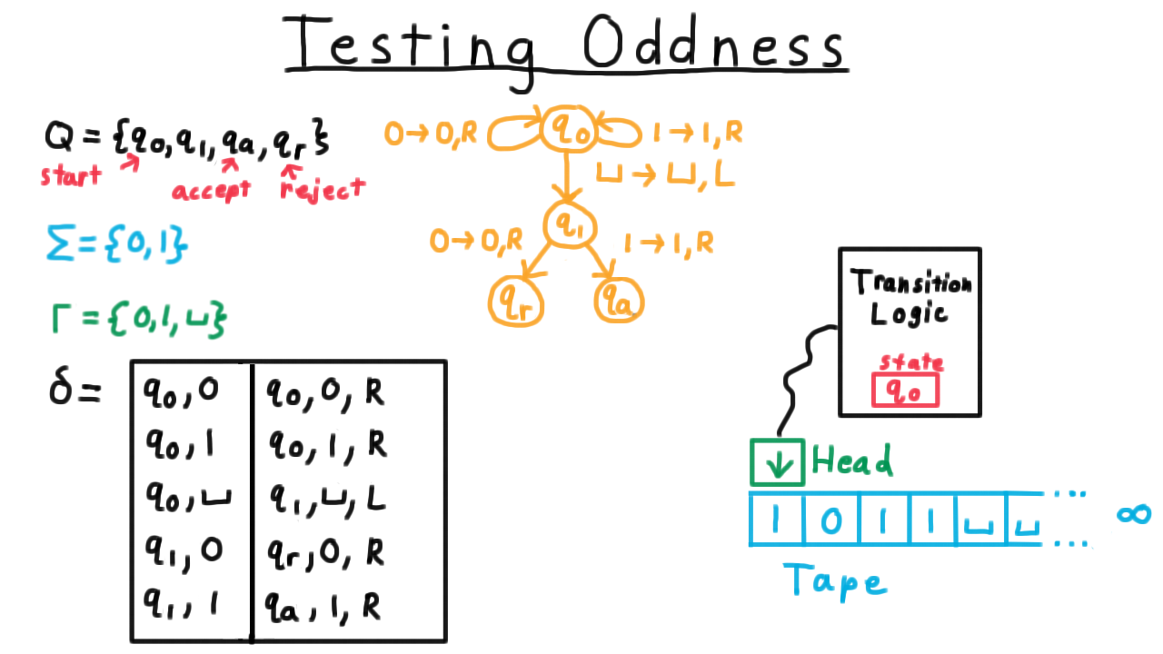
One convenient way represent the transition function, by the way, is with a state diagram, similar to what is often used for finite automata for those familiar with that model of computation. Each state gets its own vertex in a multigraph and every row of the transition table is represented as an edge. The edge gets labeled with remaining information besides the two states, that is the symbol that is read, the one that is written and the direction in which the head is moved.
See if you can trace throught the operation of the Turing machine for the input shown. If you are unsure, watch the video.
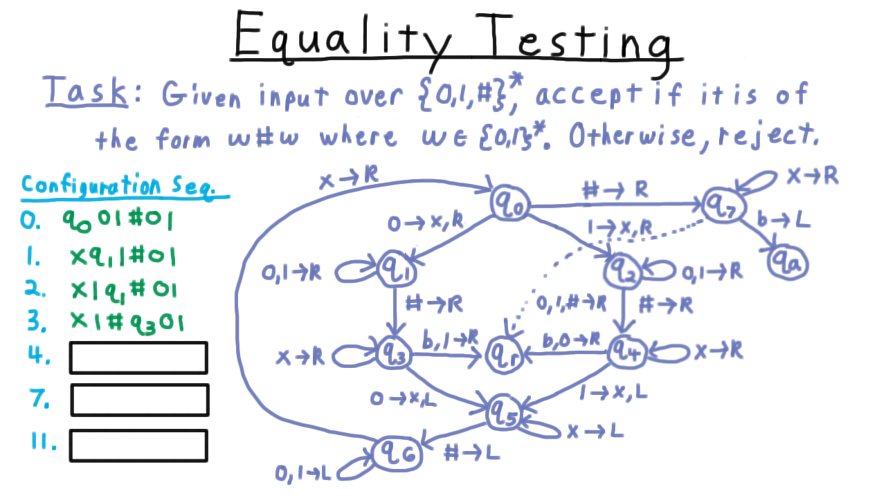
Configuration Sequences - (Udacity, Youtube)
Recall that a Turing machine always starts in the initial state and with the head at the first position on the tape. As it computes, it’s internal state, the tape contents, and the position of the head will change, but everything else will stay the same. We call this triple of state, tape content, and head position a configuration, and any given computation can be thought of as a sequence of configurations. It starts with the initial state, the input string and with the head position on the first location, and it proceeds from there.
Now, it isn’t very practical always draw a picture like this one every time that we want to refer to the configuration of a Turing machine, so we develop some notation that captures the idea.

We’ll do the same computation again, but this time we’ll write down the configuration using this notation. We write the start configuration as \(q_0\)1011. The part to the left of the state represents the contents of the tape to the left of the head. It’s just the empty string in this case. Then we have the state of the machine and then the rest of the tape contents.
After the first step, 1 is to the left of the head, we are state \(q_0\) still and ‘1’ is the string to the right. In the next, configuration ‘10’ is to the left, we are still in state \(q_0\) and ‘11’ to right,and so on and so forth.
This notation is a little awkward, but it’s convenient for typesettings. It’s also very much in the spirit of Turing machines, where all structured data must ultimately be represented as strings. If a Turing machine can handle working with data like this, then so can we.
At a slightly higher level, a whole sequence of configurations like this captures everything that a Turing machine did on a particular input, and so we will sometimes call such a sequence a computation. And actually, this representation of a computation will be central as when we discuss the Cook-Levin theorem in the section on complexity.
The Value of Practice - (Udacity, Youtube)
Next, we are going get some practice tracing though Turing machine computations and programming Turing machines. The point of these exercises is not, so that you can put on your resume that you are good at programming Turing machines. And if someone asks you in an interview to write a program to test whether an input number is prime, I wouldn’t recommend trying to draw a Turing machine state diagram. Somehow, I doubt that will land you the job.
Rather, the point is to help you convince yourself that Turing machines can do everything that we mean by computation, and if you really had to, you could program a Turing machine to do anything that your could write a procedure to do in your favorite programming language. There are two ways to convince yourself of this. One is to just practice so that you build up enough of a facility with programming them – that is to say, it becomes easy enough for you– so that it just seems intuitive that you could do anything. Another way is to show that a Turing machine can simulate the action of models that are closer to real-world computers like the Random Access Model. We’ll do that in a later lesson. But, to be able to understand these simulation arguments, you need a pretty good facility with how Turing machines work anyway, so make the most of these examples and exercises.
Equality Testing - (Udacity, Youtube)
To illustrate some of the key challenges in computing with Turing machines and how to overcome them, we’ll examine this task here, where we are given an input string, and want to tell if it is of the form w#w, where w is a binary string. In other words, we want to test whether the string to the left of the first hash is the same as the string to the right of it.
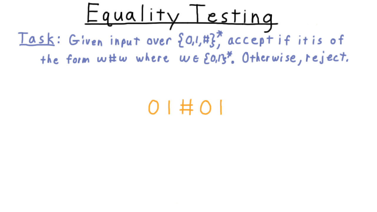
(Watch the video for an illustration on this example.)
As Turing machines go this is a pretty simple program, but as you can see here the state diagram gets a little messy. Like the Sisper textbook, I’ve used a little shorthand here in the diagram. When two symbols appear to the left of the arrow, I mean to either one of those. It’s easier than writing out a whole other edge. Also, sometimes, I will only give a direction on the right. Interpret that to mean that the tape should be left alone.
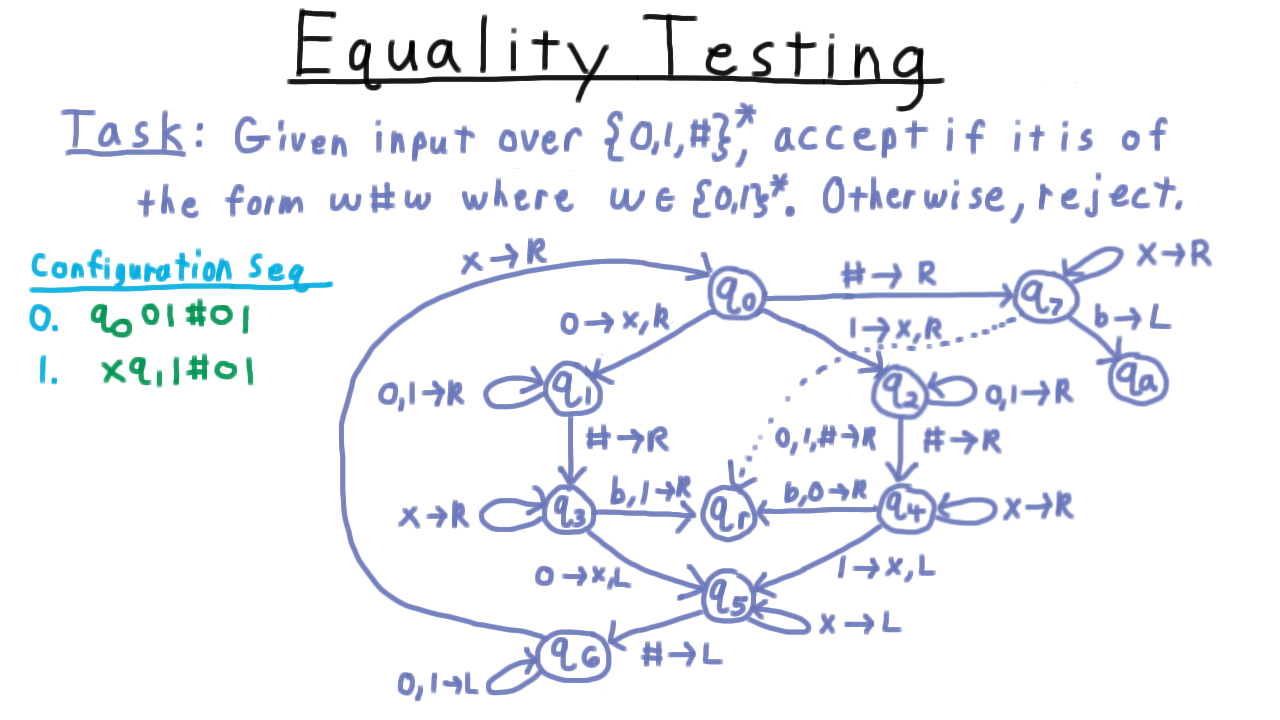
(Watch the video for an illustration of the state transitions in the diagram.)
Configuration Exercise - (Udacity)
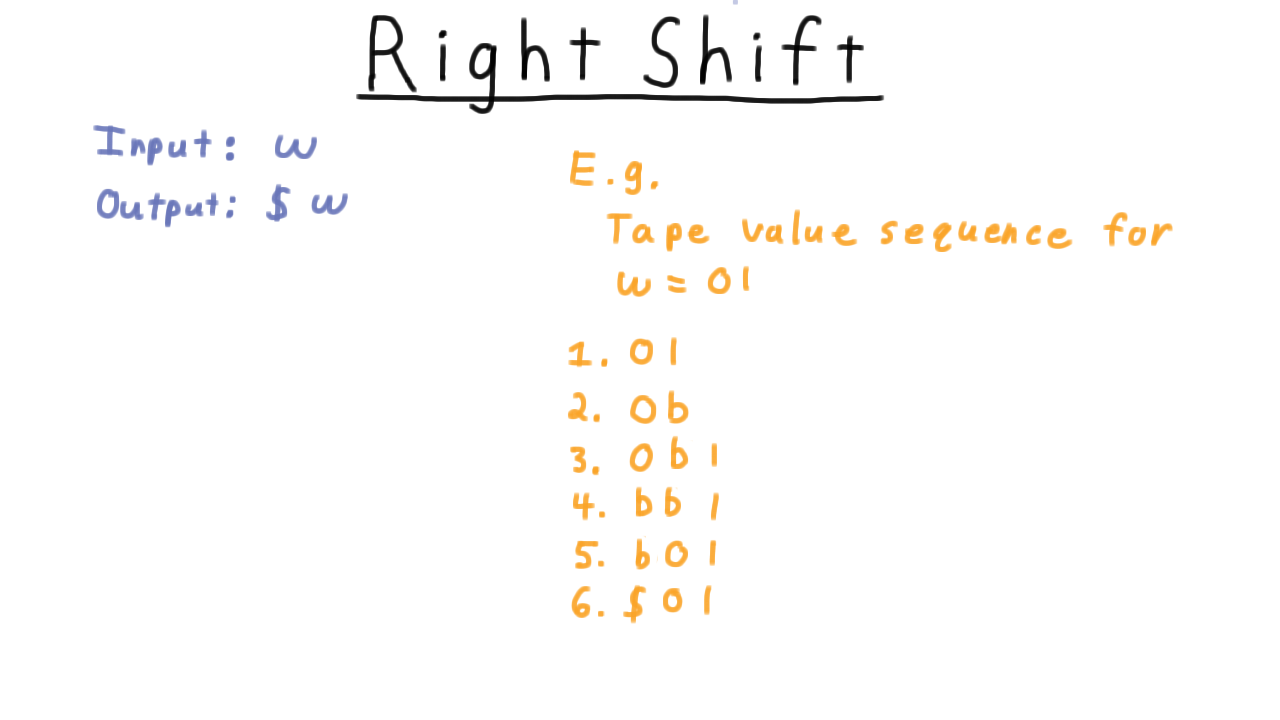
Right Shift - (Udacity)
Now, I want you to actually build a Turing machine. The goal is to right-shift the input and place a dollar sign symbol in front of the input and accept. Unlike our previous examples, accept vs. reject isn’t important here. This is more like a subroutine within a larger Turing machine that you might want to build, though you could think about it as a Turing machine that computes a function from all strings over the input alphabet to string over the tape alphabet, if you like.
Balanced Strings - (Udacity)
Language Deciders - (Udacity, Youtube)
If you completed all those exercises, then you are well on your way towards understanding how Turing machines compute, and hopefully, also are ready to be convinced that they can compute as well as any other possible machine.
Before we move onto that argument, however, there is some terminology about Turing machines and the languages that they accept and reject those that they might loop on that we should set straight. Some of the terms may seem very similar, but the distinctions are important ones and we will use them freely throughout the rest of the course, so pay close attention. First we define what it means for a machine to decide a language.
A Turing machine decides a language L if and only if accepts every x in L and rejects every x not in L.

For example, the Turing machine we just described decided the langauge L consisting of strings of the form w#w, where w is a binary string. We might also say the Turing machine computed the function that is one if x is in L and 0 otherwise. Or even just that the Turing machine computed L.
Contains a One - (Udacity)
Now for a question that is a little tricky. Consider the language that consists of all binary strings that contain a symbol 1. Does this Turing machine decide L?
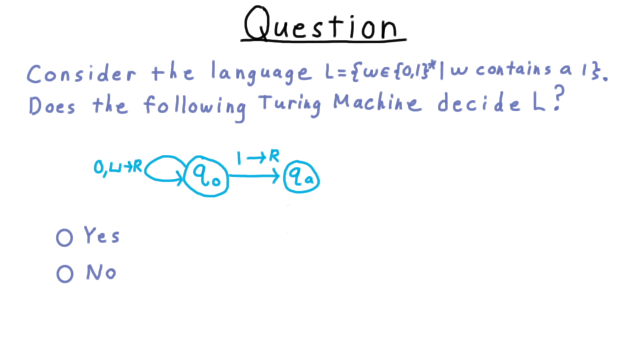
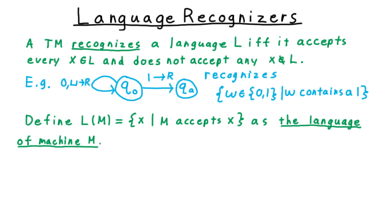
Language Recognizers - (Udacity, Youtube)
The possibility of Turing machines looping forever leads us to define the notion of a language recognizer.
We say that a Turing machine recognizes a language L iff and accepts every string in the language and does not accept every string not in the language. Thus, we can say that the Turing machine from the quiz does indeed recognize the language consisting of strings that contain a 1. It accepts those containing 1 and it doesn’t accept the others; it loops on them.

Contrast this definition with what it takes for a Turing machine to decide a language. Then it needs not only to accept everything in the language but it must reject everything else. It can’t loop like this Turing machine.
If we wanted to build a decider for this language we would need to modify the Turing machine so that it detects the end of the string and move into the reject state.
At this point, it also makes sense to define the language of a machine, which is just the language that the machine recognizes. After all, every machine recognizes some language, even if it is the empty one.
Formally, we define \(L(M)\) to be the set of strings accepted by \(M\), and we call this the language of the machine \(M\).
Conclusion - (Udacity, Youtube)
In this lesson, we examined the workings of Turing machines, and if you completed all the exercises, you should have a strong sense of how to use them to compute functions and decide languages. We’ve also seen how unlike some simpler models of computation, Turing machines don’t necessarily halt on all inputs. This forced us to distinguish between language deciders and language recognizers. Eventually, we will see how this problem of halting or not halting will be the key to understanding the limits of computation.
We’ve shown Turing machines can test equality of strings, not something that could be computed by simpler models like finite or push-down automaton that you might have seen in your undergraduate courses. But equality is a rather simple problem–can Turing machines solve the complex tasks we have our computer do. Can a Turing machines do your taxes or play a great game of chess? Next lesson, we’ll see that Turing machines can indeed solve any problem that our computers can solve and truly do capture the idea of computation.
Church-Turing Thesis - (Udacity)
Introduction - (Udacity, Youtube)
In this lecture, we will give strong evidence for the statement that
everything computable is computable by a Turing machine.
This statement is called the Church-Turing thesis, named for Alan Turing, whom we met in the previous lesson, and Alonzo Church, who had an alternative model of computation known as the lambda-calculus, which turns out to be exactly as powerful as a Turing machine. We call the Church-Turing thesis a thesis because it isn’t a statement that we can prove or disprove. In this lecture we’ll give a strong argument that our simple Turing machine can do anything today’s computers can do or anything a computer could ever do.
To convince you of the Church-Turing thesis, we’ll start from the basic Turing Machine and then branch out, showing that it is equivalent to machines as powerful as the most advanced machines today or in any conceivable future. We’ll begin by looking at multi-tape Turing machines, which in many cases are much easier to work with. And we’ll show that anything a multi-tape Turing machine can do, a regular Turing machine can do too.
Then we’ll consider the Random Access Model: a model capturing all the important capabilities of a modern computer, and we will show that it is equivalent to a multitape Turing machine. Therefore it must also be equivalent to a regular Turing machine. This means that a simple Turing machine can compute anything your Intel i7—or whatever chip you may happen to have in your computer—can.

Hopefully, by the end of the lesson, you will have understood all of these connections and you’ll be convinced that the Church-Turing thesis really is true. Formally, we can state the thesis as:
a language is “computable” if and only if it can be implemented on a Turing machine.
Simulating Machines - (Udacity, Youtube)
Before going into how single tape machines can simulate multitape ones, we will warm up with a very simple example to illustrate what is meant when we say that one machine can simulate another.
Let’s consider what I’ll call stay-put machines. These have the capability of not moving their heads in a computation step (which Turing machines, as we’ve defined them, are not allowed to do). So the transition function now includes S, which makes the head stay put. Now, this doesn’t add any additional computational capability to the machine, because I can accomplish the same things with a normal Turing machine. For every transition where the head stays put,
we can introduce a new state, and just have the head move one step right and then one step left. (Gamma here means match everything in the tape alphabet).

This puts the tape head back in the spot it started without affecting the tape’s contents. Except for occasionally taking an extra movement step, this Turing machine will operate in the same way as the stay-put machine.
More precisely, we say that two machines are equivalent
- if they accept the same inputs, reject the same inputs, and loop on the same inputs.
- considering the tape to be part of the output, equivalent machines also halt with the same tape contents.
Note that other properties of the machines (such as the number of states, the tape alphabet, or the number of steps in any given computation) do not need to be same. Just the relationship between the input and the output matters.
Multitape Turing Machines - (Udacity, Youtube)
Since having multiple tapes makes programming with Turing machines more convenient, and since it provides a nice intermediate step for getting into more complicated models, we’ll look at this Turing machine variant in detail. As shown in the figure here, each tape has its own tape head.

What the Turing machine does at each step is determined solely by its current state and the symbols under these heads. At each step, it can change the symbol under each head, and moves each head right or left, or just keeps it where it is. (With a one-tape machine, we always forced the head to move, but if we required that condition for multitape machines, the differences in tape head positions would always be even, which leads to awkwardness in programming. It’s better to allow the heads to stay put.)
Except for those differences, multitape Turing machines are the same as single-tape ones. We’ll only need to redefine the transition function. For a Turing machine with k tapes, the new transition function is
\[\delta: Q \times \Gamma^k : \rightarrow Q \times \Gamma^k \times \\{L,R,S\\}^k\]
Everything else stays the same.
Duplicate the Input - (Udacity, Youtube)
Let’s see a multitape Turing machine in action. Input always comes in on the first tape, and all the heads start at the left end of the tapes. Our task will be to duplicate this input, separated by a hash mark.

(See video for animation of the computation).
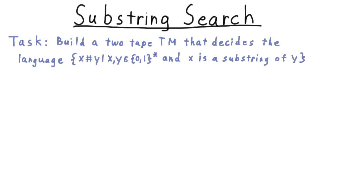
Substring Search - (Udacity)
Next, we’ll do a little exercise to practice using multitape Turing machines. Again, the point here is not so that you can put experience programming multitape Turing machines on your resume. The idea is to get you familiar with the model so that you can really convince yourself of the Church-Turing thesis and understand how Turing machines can interpret their own description in a later lesson.
With that in mind, your task is to build a two-tape TM that decides the language strings of the form x#y, where x is a substring of y. So for example, the string 101#01010 is in the language.
The second through fourth character of y match x. But on the other hand, 001#01010 is not in the language. Even though two 0s and a 1 appear in the string 01010, 001 is not a substring because the numbers are not consecutive.
Multitape SingleTape Equivalence - (Udacity, Youtube)
Now, I will argue that these enhanced multitape Turing machines have the same computational power as regular Turing machines. Multitape machines certainly don’t have less power: by ignoring all but the input tape, we obtain a regular Turing machine.
Let’s see why multitape machines don’t have any more power than regular machines.
On the left, we have a multitape Turing machine in some configuration, and on the right, we have created a corresponding configuration for a single-tape Turing machine.

On the single tape, we have the contents of the multiple tapes, with each tape’s contents separated by a hash. Also, note these dots here. We are using a trick that we haven’t used before: expanding the size of the alphabet. For every symbol in the tape alphabet of the multitape machine, we have two on the single tape machine, one that is marked by a dot and one that is unmarked. We use the marked symbols to indicate that a head of the multitape machine would be over this position on the tape.
Simulating a step of the multitape machine with the single tape version happens in two phases: one for reading and one for writing. First, the single-tape machine simulates the simultaneous reading of the heads of the multitape machines by scanning over the tape and noting which symbols have marks. That completes the first phase where we read the symbols.
Now we need to update the tape contents and head positions or markers as part of the writing phase. This is done in a second, leftward pass across the tape. (See video for an example.)
Note that it is possible that one of these strings will need to increase its length when the multitape reaches a position it hasn’t reached before. In that case, we just right-shift the tape contents to allow room for the new symbol to be written.
Once all that work is done, we return the head back to the beginning to prepare for the next pass.
So, all the information about the configuration of a multitape machine can be captured in a single tape. It shouldn’t be too hard to convince yourself that the logic of reaching and keeping track of the multiple dotted symbols and taking the right action should be as well. In fact, this would be a good for you to do on your own.
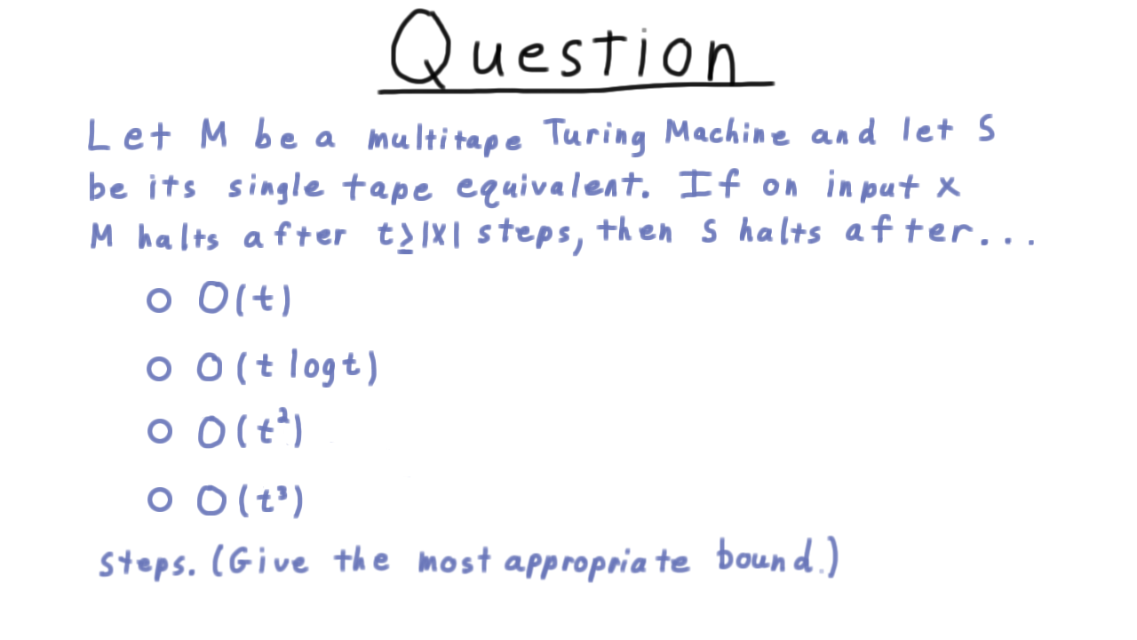
Analysis of Multitape Simulation - (Udacity)
Now for an exercise. No more programming Turing machines. Instead, I want you to try to figure out how long this simulation process takes. Let M be a multitape Turing machine and let S be its single-tape equivalent as we’ve defined it. If on input x, M halts after t steps, then S halts after… how many steps. Give the most appropriate bound. Note that we are treating the number of tapes k as a constant here.
This question isn’t easy, so just spend a few minutes thinking about it and take a guess, before watching the video answer.
RAM Model - (Udacity, Youtube)
There are other curious variants of the basic Turing machines: we can restrict them so that a symbol on a square can only be changed once, we can let them have two-way infinite tapes, or even let them be nondeterministic (we’ll examine this idea when we get to complexity). All of these things are equivalent to Turing machines in the sense we have been talking about, and it’s good to know that they are equivalent.
Ultimately, however, I doubt that the equivalence of those models does much to convince anyone that Turing machines capture the common notion of computation. To make that argument, we will show that a Turing machine is equivalent to the Random Access model, which very closely resembles the basic CPU/register/memory paradigm behind the design of modern computers.
Here is a representation of the RAM model.

Instead of operating with a finite alphabet like a Turing machine, the RAM model operates with non-negative integers, which can be arbitrarily large. It has registers, useful for storing operands for the basic operations and an infinite storage device analogous to the tape of a regular Turing machine. I’ll call this memory for obvious reasons. There are two key differences between this memory and the tape of a regular Turing machine:
- each position on this device stores a number an
- any element can be be read with a single instruction, instead of moving a head over the tape to the right spot.
In addition to this storage, the machine also contains the program itself expressed as a sequence of instructions and a special register called the program counter, which keeps track of which instruction should be executed next. Every instruction is one of a finite set that closely resembles the instructions of assembly code. For instance, we have the instruction read j, which reads the contents from the jth address on the memory and places it in register 0. Register 0, by the way, has a special status and is involved in almost every operation. We also have a write operation, which writes to the jth address in memory. For moving data between the registers, we have load, which write to \(R_0\), and store which writes from it, as well as add, which increases the number in \(R_0\) by the amount in \(R_j\). All of these operations cause the program counter to be incremented by 1 after they are finished.
To jump around the list of instructions—as one needs to do for conditionals—we have a series of jump instructions that change the program counter, sometimes depending on the value in \(R_0\).
And finally, of course, we have the halt instruction to end the program. The final value in \(R_0\) determines whether it accepts or rejects. Note that in our definition here there is no multiplication. We can achieve that through repeated addition.
We won’t have much use for the notation surrounding the RAM model, but nevertheless it’s good to write things down mathematically, as this sometimes sharpens our understanding. In this spirit, we can say that a Random Access Turing machine consists of :
- a natural number \(k\) indicating the number of registers
- and a sequence of instructions \(\Pi\).
The configuration of a Random Access machine is defined by
- the counter value, which is 0 for the halting state and indicates the next instruction to be executed otherwise.
- the register values and the values in the memory, which can be expressed as a function.
(Note that only a finite number of the addresses will contain a nonzero value, so this function always has a finite representation. We’ll use 1-based indexing, hence the domain for the tape is the natural numbers starting from one.)
Equivalence of RAM and Turing Machines - (Udacity, Youtube)
Now we are ready to argue for the equivalence of our Random Access Model and the traditional Turing machine. To translate between the symbol representation of the Turing machine and numbers of RAM, we’ll use a one-to-one correspondence E.
The blank symbol is mapped to to zero (\(E(\sqcup) = 0)so that the default value of the tape corresponds to the default value for memory.
First, we argue that a RAM can simulate a single tape Turing machine. The role of the tape played in the Turing machine will be played by the memory We'll keep track of the head position in a fixed register, say \)R_1\(. And the program and the program counter will implement the transition function. Here, I've written out in psuedocode what this might look like for the simple Turing machine shown over here, which just replaces all the ones with zeros and then halts.

Now we argue the other way: that a traditional Turing machine can simulate a RAM. Actually, we’ll create a multitape Turing machine that implements a RAM since that is a little easier to conceptualize. As we’ve seen, anything that can be done on a multitape Turing machine can be done with a single tape.

We will have one tape per register, and each tape will represent the number stored in the corresponding register.
We also have another tape that is useful for scratch work in some of the instructions that involve constants like add 55.
Then we have two tapes corresponding to the random access device. One is for input and output, and the other is for simulating the contents of the memory device during execution. Storing the contents of the random access device is the more interesting part. This is done just by concatenating the (index, values) pairs using some standard syntax like parentheses and commas.
The program of the RAM must be simulated by the state transitions of the Turing machine. This can be accomplished by having a subroutine or sub-Turing machine for each instruction in the program. The most interesting of these instructions are the ones involving memory. We simulate those by searching the tape that stores the contents of the RAM for one of these pairs that has the proper index and then reading or writing the value as appropriate. If no such pair is found, then the value on the memory device must be zero.
After the work of the instruction is completed, the effect of incrementing the program counter is achieved by transitioning to the state corresponding to the start of the next instruction. That is, unless the instruction was a jump, in which case that transition is effected. Once the halt instruction is executed the contents of the tape simulating the random access device are copied out onto the I/O tape.
RAM Simulation Running Time - (Udacity)
Given this description about how a traditional Turing machine can simulate a Random Access Model, I want you to think about how long this simulation takes. Let R be a random access machine and let M be its multi-tape equivalent. We’ll let n be the length of the binary encoding of the input to R and let t be the number of steps taken by R. Then M takes how long to simulate R?
This is a tough question, so I’ll give you a hint: the length of the representation of a number increases by at most a constant in each step of the random access machine R.

Conclusion - (Udacity, Youtube)
Once you know that a Turing machine can simulate a RAM, then you know it can simulate a standard CPU. Once you can simulate a CPU, you can simulate any interpreter or compiler and thus any programming language. So anything you can run on your desktop computer can be simulated by a Turing machine.
What about multi-core, cloud computing, probabilistic, quantum and DNA computing? We won’t do it here, but you can prove Turing machines can simulate all those models as well. The Church-Turing thesis has truly stood the test of time. Models of computation have come and go but none have been any match for the Turing machine.
Why should we care about the Church-Turing thesis? Because there are problems that Turing machines can’t solve. We argued this with counting arguments in the first lecture and will give specific examples in future lectures. If these problems can’t be solved by Turing machines they can’t be solved by any other computing device.
To help us describe specific problems that one cannot compute, in the next lecture we discuss two of Turing’s critical insights: that a computer program can be viewed as data—as part of the input to another program—and that one can have a universal Turing machine that can simulate the code of any other computer: one machine to rule them all.
Universality - (Udacity)
Introduction - (Udacity, Youtube)
In 1936, when Alan Turing wrote his famous paper “On Computable Numbers”, he not only created the Turing machine but had a number of other major insights on the nature of computation. Turing realized that the computer program itself could also be considered as part of the input. There really is no difference between the program and data. We all take that for a given today: we create computer code in a file that gets stored on the computer no differently than any other type of file. And data files often have computer instructions embedded in them. Even modern computer fonts are basically small programs that generate readable characters at arbitrary sizes.
Once he took the view of program code as data, Turing had the beautiful idea that a Turing machine could simulate that code. There is some fixed Turing machine, a universal Turing machine, that can simulate the code of any other Turing machine. Again, this is an idea that we take for granted today, as we have interpreters and compilers that can run the code of any programming language. But, back in Turing’s day, this idea of a universal machine was the major breakthrough that allowed Turing, and will allow us, to develop problems that Turing machines or any other computer cannot solve.
Encoding a Turing Machine - (Udacity, Youtube)
Before we can simulate or interpret a Turing machine, we first have to represent it using a string. Notice that this presents an immediate challenge: our universal Turing machine must use a fixed alphabet for its input and have a fixed number of states, but it must be able to simulate other Turing machines with arbitrarily large alphabets and an arbitrary numbers of states. As we’ll see, one solution is essentially to enumerate all the symbols and states and represent them in binary. There are lots of ways to do this: the way we’re going to do it is a compromise of readability and efficiency.
Let \(M\) be a Turing machine with states \(Q = \{q_0,\ldots q_{n-1}\}\) and tape alphabet \(\Gamma = \{a_1, \ldots a_m \}\). Define \(i\) and \(j\) so that \(2^i\) is at least the number of states and \(2^j\) is at least the number of tape symbols. Then we can encode a state \(q_k\) as the concatenation of the symbol q with the string w, where w is the binary representation of \(k\). For example, if there are 6 states, then we need three bits to encode all the states. The state \(q_3\) would be encoded as the string q011. By convention, we make
- \(q_0\) the initial state,
- \(q_1\) the accept state,
- \(q_2\) the reject state.
We use an analogous strategy for the symbols, encoding \(a_k\) as the symbol a followed by the string w, where w is the binary representation of k.
For example, if there are 10 symbols, then we need four bits to represent them all. If \(a_5\) is the star symbol, we would be encode that symbol as a0101.
Let’s see an encoding for an example.

This example decides whether the input consists of a number of zeros that is a power of two. To encode the Turing machine as a whole we really just need to encode its transition function. We’ll start by encoding the black edge from the diagram. We are going from state zero, seeing the symbol zero, and we go to state three, we write symbol 0 and we move the head to the right.
Remember that the order here is input state, input symbol. Then output state, output symbol, and finally direction.
Encoding Quiz - (Udacity)
Now, I’m not going to write out all the rest of the transitions, but I think it would be a good idea for you to do one more. So use this red box here to encode this red transition.

Building a Universal Turing Machine - (Udacity, Youtube)
Now, we are ready to describe how to build this all-powerful universal Turing machine. As input to the universal machine, we will give the encoding of the input and the encoding of M, separated by a hash. We write this as
The goal is to similate M’s execution when given the input w, halting in an accept or reject state, or not halting at all, and ultimately outputing the encoding of the output of M on w when M does halt. We’ll describe a 3-tape Turing machine that achieves this goal of simulating M on w.
The input comes in on the first tape. First, we’ll copy the description of the machine to the second tape and copy the initial state to the third tape. For example, the tape contents might end up like this.

The we rewind all the heads and begin the second phase.
Here, we search for the appropriate tuple in the description of the machine. The first element has to match the current state stored on tape three, and the symbol part has to match the encoding on the tape 1. If no match is found, then we halt the simulation and put the universal machine in an accepting or rejecting state according to the current state of the machine being interpreted. If there is a match, however, then we apply the changes to the first tape and repeat.

Actually, interpreting a Turing machine description is surprisingly easy.
We’ve just seen how Turing machines are indeed reprogrammable just like real-world computers. This lends further support to the Church-Turing thesis, but it also has significance beyond that. Since the input to a Turing machine can be interpreted as a Turing machine, this suggest that programs are a type of data. But arbitrary data can also be interpretted as a (possibly invalid) Turing machine. So is there any difference between data and program? Perhaps, we can leave this question for the philosophers.
Abstraction - (Udacity, Youtube)
At this point, the character of our discussion of computability is going to change signficantly. We’ve established the key properties of Turing machines: that they can do anything we mean by computation and that we can pass a description of a Turing machine to a Turing machine as input for it to simulate. With these points established, we won’t need to talk about the specifics of Turing machines much anymore. There will be little about tapes or states, transitions or head positions. Instead, we will think about computation at a very high level, trusting that if we really had to, we could write out the Turing machine to do it. If we need to write out code, we will do so only in pseudocode or with pictures.
What is there left to talk about? Well, remember from the very first lesson that we argued that not all functions are computable, or as we later said, not all languages can be decided by Turing machines. We’re now in a good position to talk about some of these undecidable languages. We had to wait until we established the universality of Turing machines because these languages are going to consist of strings that encode Turing machines. The rest of the lesson will review the definitions of recognizability and decidability, and then we’ll talk about the positive side of the story: the languages about Turing machines that we CAN decide or recognize. As we’ll see, there are plenty that we can’t.
Language Recognizers - (Udacity, Youtube)
Recall that a Turing machine recognizes a language if it accepts every string in the language and does not accept anything that is not in the language. It could either reject or loop. This Turing machine here recognized the language of binary strings containing a 1, but it looped on those that don’t contain a 1.

In order to decide a language, the Turing machine must not only accept every string in the language but it must also explicitly reject every string that is not in the language. This machine achieves that by not looping on the blanks.
Recognizability and Decidability - (Udacity, Youtube)
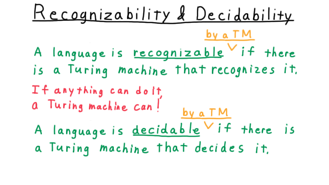
Ultimately, however, we are not interested in whether a particular Turing machine recognizes or decides a language; rather we are interested in whether there is a Turing machine that can recognize or decides the language.
Therefore, we say that a language is recognizable if there is a Turing machine that recognizes it, and we say that a language is decidable if there is a Turing machine that decides it.
A language is recognizable if there is a Turing machine that recognizes it.
A language is decidable if there is a Turing machine that decides it.
Now, looking at this someone might object, “Shouldn’t we say ‘recognizable by a Turing machine’ and ‘decidable by a Turing machine’?” Of course, we could and the statements would still be true. But we don’t, the reason being that we strongly believe that if anything can do it a Turing machine can! That’s the Church-Turing thesis.
In an absolute sense, we believe that a language is only recognizable by anything if a Turing machine can recognize it and a language is only decidable by anything if a Turing machine can decide it, and we use terms that reflect that belief.
Now other terms are sometimes used instead of recognizable and decidable. Some say that Turing machines compute languages, so to go along with that they say that languages are computable if they there is a Turing machine that computes it. Another equivalent term for decidable is recursive. Mathematicians often prefer this word.
And those who use that term will refer to recognizable languages as recursively enumerable. Some also call these languages Turing-acceptable and semi or partially decidable.
We should also make clear the relationship between these two terms. Clearly, if a language is decidable, then it is also recognizable; the same Turing machine works for both. It feels like it should also be true that if a language is recognizable and its complement is also recognizable, then the language is decideable. This is true, but there is a potential pitfall here that we need to make sure to avoid.
Decidability Exercise - (Udacity)
Suppose that we are given one machine \(M_1\) that recognizes a language \(L\) and another \(M_2\) that recognizes \(\overline\{L\}\). If we were to ask your average programmer to use these machines to decide the language, his first guess might go something like this.
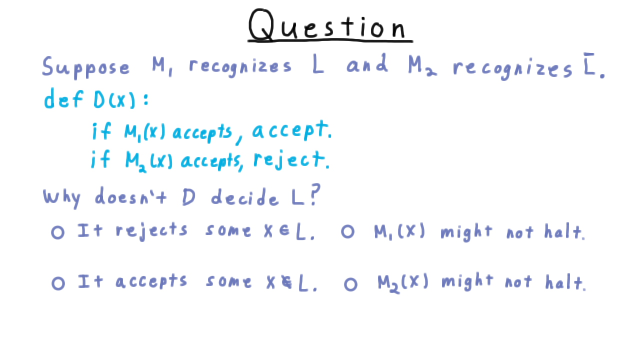
This program will not decide L, however, and I want you to tell me why. Check the best answer.
Alternating Machines - (Udacity, Youtube)
Here is the alternating trick in some more detail. Suppose that \(M_1\) recognizes a language and \(M_2\) recognizes its complement. We want to decide the language.
In psuedocode, the alternating strategy might look like this.
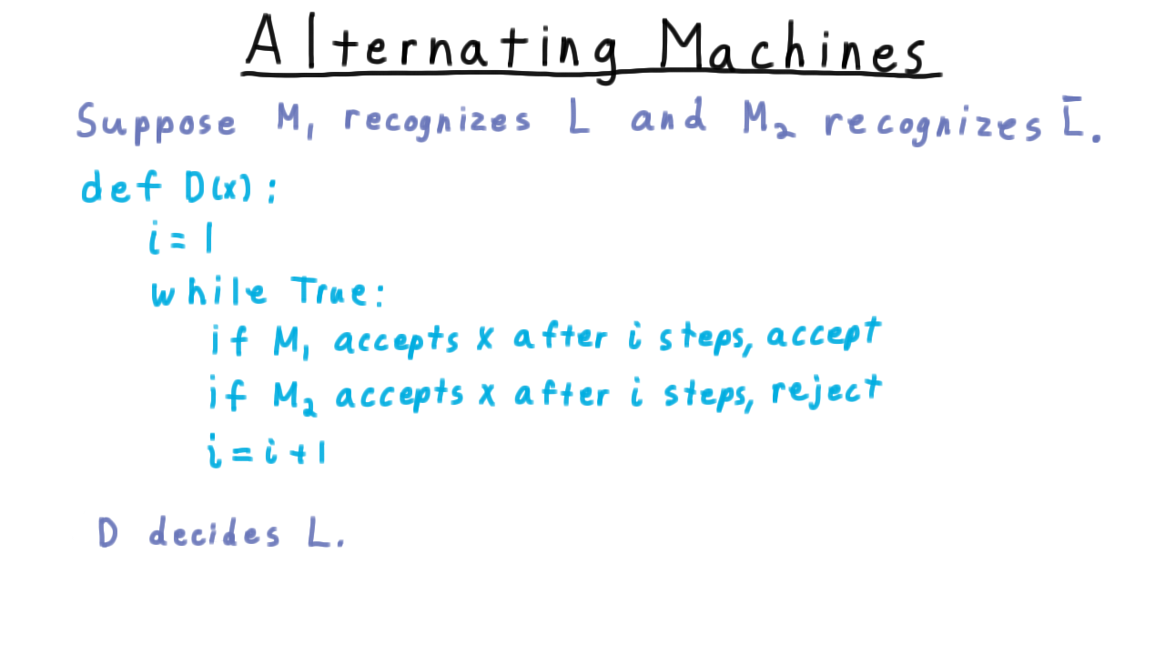
In every step, we execute both machines one more step than in the previous iteration. Note that it doesn’t matter if we save the machines configuration and start where we left off or start over. The question is whether we get the right answer, not how fast. The string has to be either in \(L\) or in \(\overline\{L\}\), so one of these has to halt after some finite number of steps, and when \(i\) hits that value, this program will give the right answer.
Overall then, we have the following theorem.
A language L is decidable if and only if L and its complement are both recognizable.
Counting States - (Udacity)
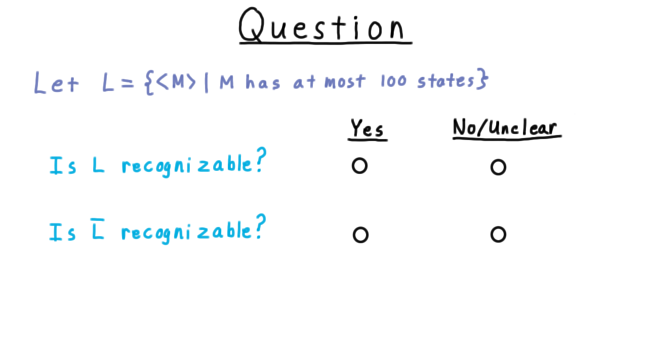
Now we’re going to go through a series of languages and try to figure out if they and their complements are recognizable. First, let’s examine the set of strings that describe a Turing machine that has at most 100 states. You can assume the particular encoding for Turing machines that we used, but any encoding will serve the same purpose.
Indicate whether you think that L is recognizable and whether L complement is recognizable. We don’t have a way proving that a language is not recognizable yet, so I’ve labeled the “No” option as unclear.
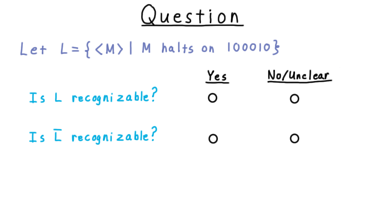
Halting on 34 - (Udacity)
Next, we consider the set of Turing machines that halt on the number 34 written in binary. Indicate whether L and L complement are recognizable.
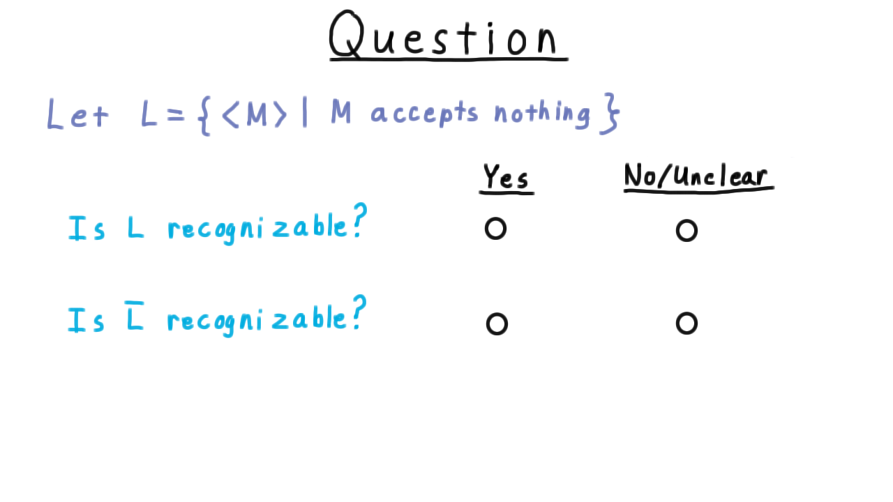
Accepting Nothing - (Udacity)
Let’s consider another language, this time the set of Turing machine descriptions where the Turing machine accepts nothing.
Tell me: are either L or L complement recognizable?
Dovetailing - (Udacity, Youtube)
Here is the dovetailing trick, which let’s you run a countable set of computations all at once. We’ll illustrate the technique for the case where we are simulating a machine M on all binary strings with this table here.
Every row in the table corresponds to a computation or the sequence of configurations the machine goes through for the given input. Simulating all of these computation means hitting every entry in this table. Note that we can’t just simulate M on the empty string first or we might just keep going forever, filling out the first row and never getting to the second. This is the same problem that we encountered when trying to show that a countable union of countable sets is countable, or that the set of rational numbers is countable.
And the solution is the same too. We go diagonal by diagonal, first simulating the first computation for one step. Then the second computation for one step and the first computation for two steps, etc. Eventually every configuration in the table is reached.
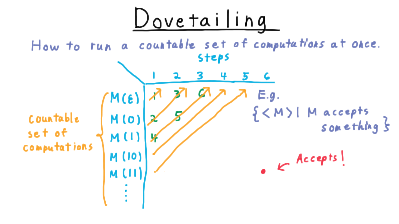
Thus, if we are trying to recognize the language of Turing machine descriptions where the Turing machine accepts something, then a Turing machine in the language must accept some string after finite number of steps.
This will correspond to some some entry in the table, so we eventually reach it and accept.
Always Halting - (Udacity)
Let’s consider one last language, the set of descriptions of Turing machines that halt on every input. Think carefully, and indicate whether you think that either L or L complement is recognizable.

Conclusion - (Udacity, Youtube)
In this and the previous lessons, we’ve developed a set of ideas and definitions that sets the stage for understanding what we can and cannot solve on a computer.
- We’ve seen the Turing machine, an amazingly simple model that can only move a tape back and forth while reading and writing on that tape.
- We’ve seen that despite it’s simplicity this model captures the full power of computers now and forever.
- We’ve seen how to consider Turing machine programs as data themselves and create a universal Turing machine that can simulate those programs.
- And at the end of this lesson, we saw some languages defined using program as data that don’t seem to be easily decidable.
In the next lecture we will show how to prove many languages cannot be solved by a Turing machine, including the most famous one, the halting problem.
Undecidability - (Udacity)
Introduction - (Udacity, Youtube)
As a computer scientist, you have almost surely written a computer program that just sits there spinning its wheels when you run it. You don’t know whether the program is just taking a long time or if you made some mistake in the code and the program is in an infinite loop. You might have wondered why nobody put a check in the compiler that would test your code to see whether it would stop or loop forever. The compiler doesn’t have such a check because it can’t be done. It’s not that the programmers are not smart enough, or the computers not fast enough: it is just simply impossible to check arbitrary computer code to determine whether or not it will halt. The best you can do is simulate the program to know when it halts, but if it doesn’t halt, you can never be sure if it won’t halt in the future.
In this lesson we’ll prove this amazing fact and beyond, not only can you not tell whether a computer halts, but you can’t determine virtually anything about the output of a computer. We build up to these results starting with a tool we’ve seen from our first lecture, diagonalization.
Diagonalization - (Udacity, Youtube)
The diagonalization argument comes up in many contexts and is very useful for generating paradoxes and mathematical contradictions. To show how general the technique is, let’s examine it in the context of English adjectives.
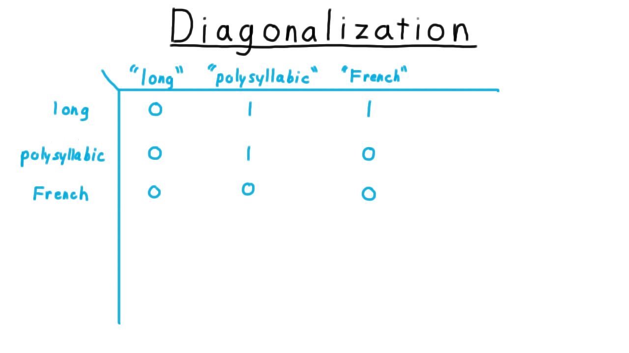
Here I’ve created a table with English adjectives both as the rows and as the columns. Consider the row to be the word itself and the column to be the string representation of the word. For each entry, I’ve written a 1 if the row adjective applies to the column representation of the word. For instance, “long” is not a long word, so I’ve written a 0. “Polysyllabic” is a long word, so I’ve written a 1. “French” is not a French word, it’s an English word, so I’ve written a 0. And so forth.
So far, we haven’t run into any problems. Now, let’s make the following definition: a heterological word is a word that expresses a property that its representation does not possess. We can add the representation to the table without any problems. It is a long, polysyllabic, non-French word. But when we try to add the meaning to the table, we run into problems. Remember: a heterological word is one that express a property that its representation does not posseses. “Long” is not a long word, so it is heterological. “Polysyllabic” is a polysyllabic word, so it is not heterological, and “French” is not a French word, so it is heterological.
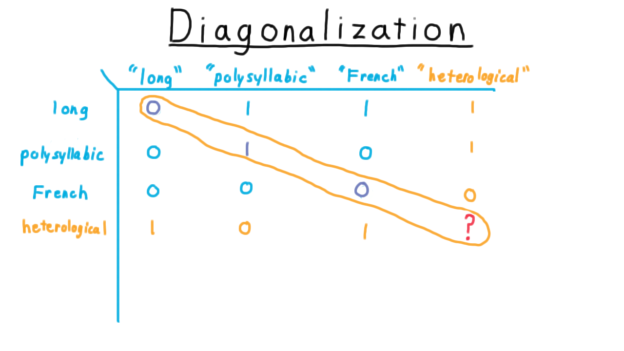
What about “heterological,” however? If we say that it is heterological (causing us to put a 1 here), then it applies to itself and so it can’t be heterological. On the other hand, if we say it is not heterological (causing us to put a zero here), then it doesn’t apply to itself and it is heterological. So there really is no satisfactory answer here. Heterological is not well-defined as an adjective.
For English adjectives, we tend to simply tolerate the paradox and politely say that we can’t answer that question. Even in mathematics the polite response was simply to ignore such questions until around the turn of the 20th century when philosophers began to look for a more solid logical foundations for reasoning and for mathematics in particular.
Naively, one might think that a set could be an arbitrary collection. But what about the set of all sets that do not contain themselves? Is this set a member of itself or not? This paradox posed by Bertrand Russell wasn’t satisfactorily resolved until the 1920s with the formulation of what we now call Zermelo-Fraenkel set theory.
Or from mathematical logic, consider the statement, “This statement is false.” If this statement is true, then it says that it is false. And if this statement is false, then it says so and should be true. It turns out that falsehood in this sense isn’t well-defined mathematically.
At this point, you’ve probably guessed where this is going for this course. We are going to apply the diagonalization trick to Turing machines.
An Undecidable Language - (Udacity, Youtube)
Here is the diagonalization trick applied to Turing machines. We’ll let \(M_1, M_2, \ldots \), be the set of all Turing machines. Turing machines can be described with strings, so there are a countable number of them and therefore such an enumeration is possible. We’ll create a table as before. I’ll define the function
\[ f(i,j) = \left\{ \begin{array}{ll} 1 & \mathrm{if} \; M_i \; \mathrm{accepts }\; < M_j > \\\\ 0 & \mathrm{otherwise} \end{array}\right. \]
For this example, I’ll fill out the table in some arbitrary way. The actual values aren’t important right now.

Now consider the language L, consisting of string descriptions of machines that do not accept their own descriptions. I.e.
\[ L = \{ < M > | < M > \notin L(M) \}. \]
Let’s add a Turing machine \(M_L\) that recognizes this language to the grid.

Again we run into a problem. The row corresponding to \(M_L\) is supposed to have the opposite values of what is on the diagonal. But what about the diagonal element of this row? What does the machine do when it is given its own description? If it accepts itself, then \(< M_L >\) is not in the language \(L\), so \(M_L\) should have accepted itself. On the other hand, if \(M_L\) does not accept its string representation, then \(< M_L >\) is in the language \(L\), so \(M_L\) should have accepted its string representation!
Thankfully, in computability, the resolution to this paradox isn’t as hard to see as in set theory or mathematical logic. We just conclude that the supposed machine \(M_L\) that recognizes the language L doesn’t exist.
Here is natural to object: “Of course, it exists. I just run M on itself and if it doesn’t accept, we accept.” The problem is that M on itself might loop, or it just might run for a very long time. There is no way to tell the difference.
The end result, then, is that the language L of string descriptions of machines that do not accept their own descriptions is not recognizable.
Recall that in order for a language to be decidable, both the language and its complement have to be recognizable. Since L is not recognizable, it is not decidable, and neither is it’s complement, the language where the machine does accept its own description. We’ll call this D_TM, D standing for diagonal,
\[D_{TM} = \{ < M > | < M > \in L(M)\} \]
These facts are the foundation for everything that we will argue in this lesson, so please make sure that you understand these claims.
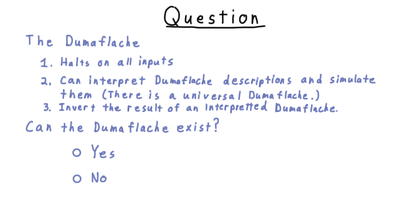
Dumaflaches - (Udacity)
If you think back to the diagonalization of Turing machines, you will notice that we hardly referred to the properties of Turing machines at all. In fact, except at the end, we might as well have been talking about a different model of computation, say the dumaflache. Perhaps, unlike Turing machines, dumaflaches halt on every input. These models exist. A model that allowed one step for each input symbol would satisfy this requirement.
How do we resolve the paradox then? Can’t we just build a dumaflache that takes the description of a dumaflache as input and then runs it on itself? It has to halt, so we can reject it if accepts and accept if it rejects, achieving the needed inversion. What’s the problem? Take a minute to think about it.
Mapping Reductions - (Udacity, Youtube)
So far, we have only proven that one language is unrecognizable. One technique for finding more is mapping reduction, where we turn an instance of one problem into an instance of another.
Formally, we say
A language \(A\) is mapping-reducible to a language \(B\) ( \(A \leq_M B\) ) if there is a computable function \(f\) where for every string \(w\),
\[w \in A \Longleftrightarrow f(w) \in B.\]
We write this relation between languages with the less-than-or-equal-to sign with a little M on the side to indicate that we are refering to mapping reducibility.
It helps to keep in your mind a picture like this.
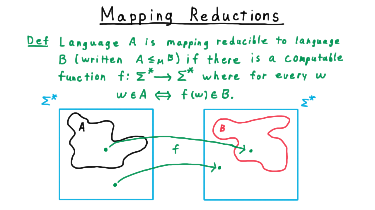
On the left, we have the language \(A\), a subset of \(\Sigma^*\) and the right we have the language \(B\), also a subset of \(\Sigma^*\).
In order for the computable function \(f\) to be a reduction, it has to map
- each string in \(A\) to a string in \(B\).
- each string not in \(A\) to a string not in \(B\).
The mapping doesn’t have to be one-to-one or onto; it just has to have this property.
Some Trivial Reductions - (Udacity, Youtube)
Before using reductions to prove that certain languages are undecidable, it sometimes helps to get some practice with the idea of a reduction itself–as a kind of warm-up. With this in mind, we’ve provided a few programming exercises. Good luck!
EVEN <= {’Even’} - (Udacity)
{’John‘} <= Complement of {’John’} - (Udacity)
{’Jane’} <= HALT - (Udacity)
Reductions and (Un)decidability - (Udacity, Youtube)
Now that we understanding reductions, we are ready to use them to help us prove decidability and even more interestingly undecidability.
Suppose then that we have a language \(A\) that reduces to \(B\) (i.e. \( A\leq_M B\) ), and, let’s say that I want to know whether some string \(x\) is in \(A\).
If there is a decider for \(B\), then I’m in luck. I can use the reduction, which is a computable function, that takes in the one string and outputs another. I just need to feed in \(x\), take the output, and feed that into the decider for \(B\). If \(B\) accepts, then I know that \(x\) is in \(A.\) If \(B\) rejects, then I know that it isn’t.
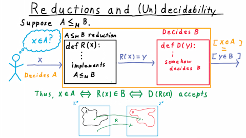
This works because by the definition of a reduction \(x\) is in \(A\) if and only if \(R(x)\) is in \(B\). And by the definition of a decider this is true if and only if \(D\) accepts \(R(x)\). Therefore, the output of \(D\) tells me whether \(x\) is in \(A.\) If I can figure out whether an arbitrary string is in \(B\), then by the properties of the reduction,this also lets me figure out whether a string is in \(A\). We can say that the composition of the reduction with the decider for \(B\) is itself a decider for \(A.\)
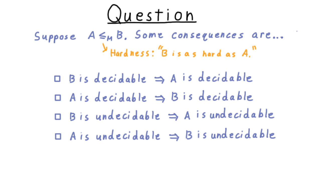
Thus, the fact that \(A\) reduces to \(B\) has four important consequences for decidability and recognizability. The easiest to see are
- If \(B\) is decidable, then \(A\) is also decidable. (As we’ve seen we can just compose the reduction with the decider for \(B.\))
- If \(B\) is recognizable, then \(A\) is also recognizable. (Same logic as above.)
The other two consequences are just the contrapositives of these.
- If \(A\) is undecidable, then B is undecidable. (This composition of the reduction and the decider for B can’t be a decider. Since we are assuming that there is a reduction, the only possibility is that the decider for B doesn’t exist. Hence, B is undecidable.)
- If \(A\) is unrecognizable, then B is unrecognizable. (Same logic as above)
Remember the Consequences - (Udacity)
Let’s do a quick question on the consequences of there being a reduction between two languages.
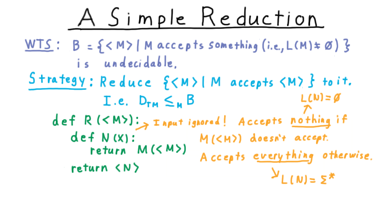
A Simple Reduction - (Udacity, Youtube)
Now we are going to use a simple reduction to show that the language \(B\), consisting of the descriptions of Turing machines that accept something, i.e.
\[ B = \{ < M > | \; L(M) \neq \emptyset \},\]
is undecidable.
Our strategy is to reduce the diagonal language to it. In other words, we’ll argue that deciding \(B\) is at least as hard as deciding the diagonal language. Since we can’t decide the diagonal language, we can’t decide \(B\) either.
Here is one of many possible reductions.
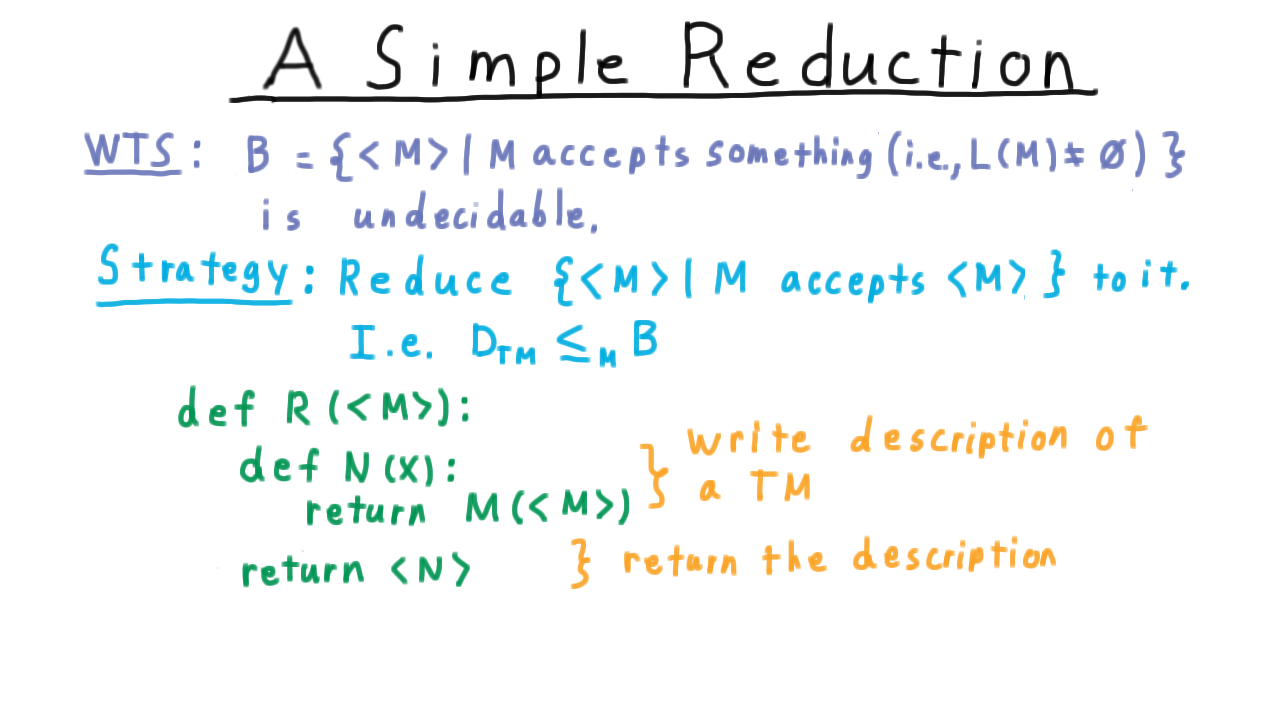
The reduction is a computable function whose input is the description of a machine M, and it’s going to build another machine N in this python-like notation. First, we write down the description of a Turing machine by defining this nested function. Then we return that function. An important point is that the reduction never runs the machine N: it just writes the program for it!
Note here that, in this example, N totally ignores the actual input that is given to it. It just accepts if M(
In other words, the language of N will be the empty set in one case and Sigma-star in the other. A decider for B would be able to tell the difference, and therefore tell us whether M accepted its own description. Therefore, if B had a decider, we would be able to decide the diagonal language, which is impossible. So B cannot be decidable.
The Halting Problem - (Udacity, Youtube)
Next, we turn to the question of halting. As we have seen, not being able to tell whether a program will halt or not plays a central role in the diagonalization paradox, and it is at least partly intuitive that we can’t tell whether a program is just taking a long time or if it will run forever. It shouldn’t be surprising, then, that given an arbitrary program-input pair, we can’t decide whether the program will halt on that input. But actually, the situation is much more extreme. We can’t even decide if a program will halt when it is given no input at all: just the empty string.
Let’s go ahead prove this:
The language of descriptions of Turing machines that halt on the empty string, i.e.
\[ H_{TM} = \{ < M > |\; M \; \mathrm{halts}\; \mathrm{on} \; \epsilon\}\]
is undecidable.
We’ll do this by reducing from the diagonal language. That is, we’ll show the halting problem is at least as hard as the diagonal problem. Here is one of many possible reductions.
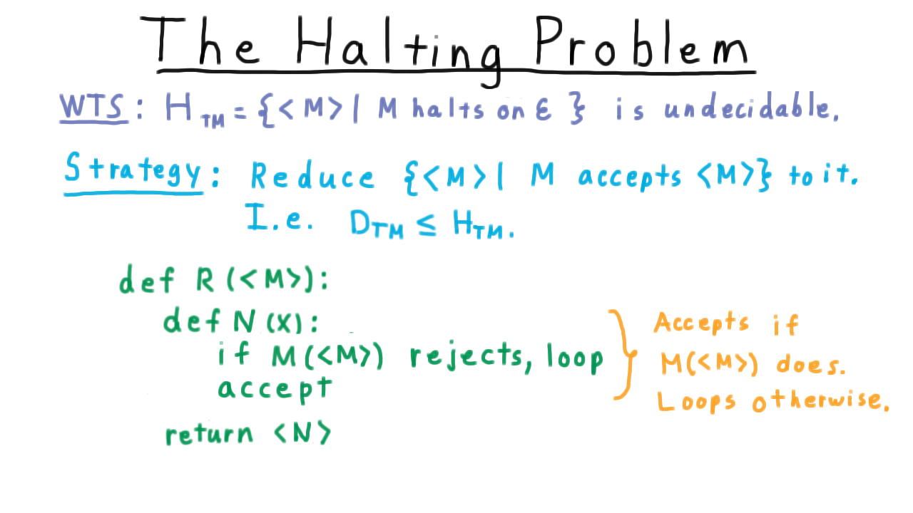
The reduction creates a machine N that simply ignores its input and runs M on itself. If M rejects itself, then N loops. Otherwise, N accepts.
At this point it might seem we’ve just done a bit of symbol manipulation but let’s step back and realize what we’ve just seen. We showed that no Turing machine can tell whether or not a computer program will halt or remain in a loop forever. This is a problem that we care about it and we can’t solve it on a Turing machine or any other kind of computer. You can’t solve the halting problem on your iPhone. You can’t solve the halting problem on your desktop, no matter how many cores you have. You can’t solve the halting problem in the cloud. Even if someone invents a quantum computer, it won’t be able to solve the halting problem. To misquote Nick Selby: “If you want to solve the halting problem, you’re at Georgia Tech but you still can’t do that!”
Filtering - (Udacity, Youtube)
So far, the machines we’ve made in our reductions (i.e. the \(N\)s) have been relatively uncomplicated: they all either accepted every string or no strings. Unfortunately, reductions can’t always be done that way, since the machine that always loops and the machine that always accepts might both be in or both not be in the language we’re reducing to. In these cases, we need \(N\) to pay attention to its input. Here is an example where we will need to do this: the language of descriptions of Turing machine where the Turing machine accepts exactly one string, i.e.
\[ S = \{ < M > |\; |L(M)| = 1 \}. \]
It doesn’t make much of a difference which undecidable language we reduce from, so this time we will reduce from the halting problem to \(S\). Again, there are many possible reductions. Here is one.
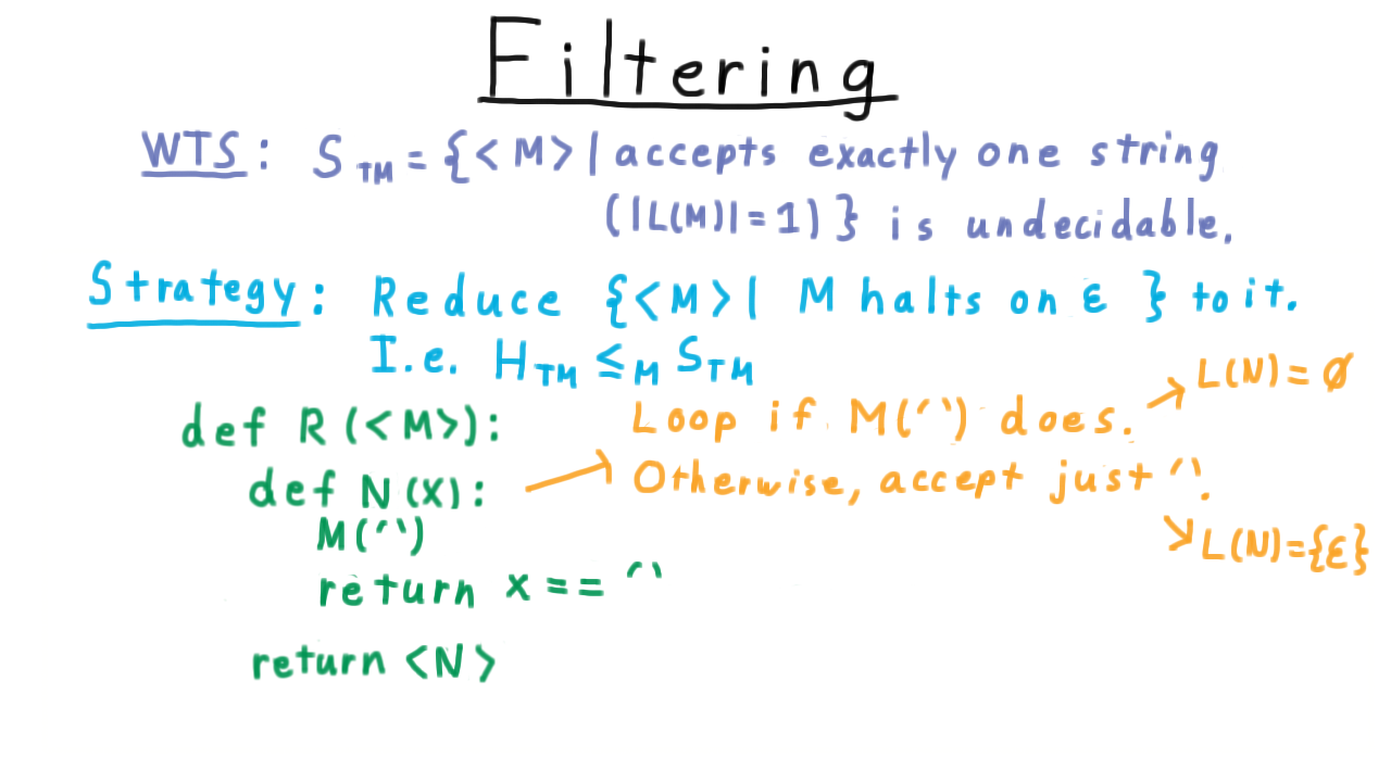
We run the input machine \(M\) on the empty string. If \(M\) loops, then so will \(N\). We don’t accept one string, we accept none. On the other hand, if \(M\) does halt on the empty string, then we make \(N\) act like a machine in the language \(S.\) The empty string is as good as any, so we’ll test to see if \(N\)’s input \(x\) is equal to that and accept or reject accordingly. This works because if \(M\) halts on the empty string, then \(N\) accepts just one string–the empty one–and so is in \(S\). On the other hand, if M doesn’t halt on the empty string, then N won’t halt on (and therefore won’t accept) anything, and therefore N isn’t in L.
In the one case, the language of \(N\) is the empty string. In the other case, the language of \(N\) is the empty set. A decider for the language \(S\) can tell the difference, and therefore we’d be able to decide if \(M\) halted on the empty string or not. Since this is impossible, a decider for \(S\) cannot exist.
Not Thirty-Four - (Udacity)
Now you get a chance to practice doing reductions on your own. I’ve been using a python-like syntax in the examples, so this shouldn’t feel terribly different. I want you to reduce the language LOOP to the language L of Turing machines that do not accept 34 in binary.
As we’ll see later in the lesson, it’s not possible for the Udacity site to perfectly verify your software, but if you do a straightforward reduction, then you should pass the tests provided.
\(0^n 1^n\) - (Udacity)
Now for a slightly more challenging reduction. Reduce \(H_\{™\}\) to the language L of Turing machines that accept strings of the form \(0^n1^n\).
Which Reductions Work? - (Udacity)
We’ve seen a few examples, and you’ve practiced writing reductions of your own at this point. Now, I want you to test your understanding by telling me which of the following statements about these two languages is true. Think very carefully.
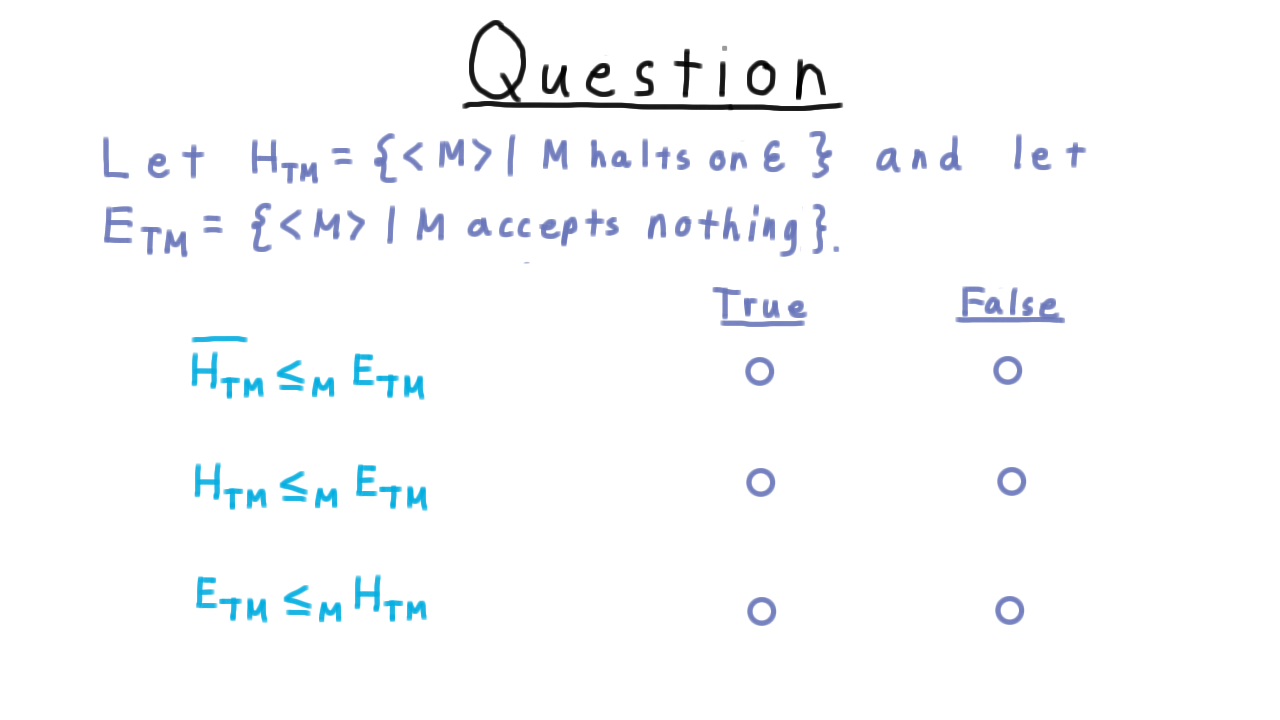
Rice’s Theorem - (Udacity, Youtube)
Once you have gained enough practice, these reductions begin to feel a little repetitive and it’s natural to wonder whether there is a theorem that would capture them all. Indeed, there is, and it is traditionally called Rice’s theorem after H.G. Rice’s 1953 paper on the subject. This is a very powerful theorem, and it implies that we can’t say anything about a computer just based on the language that it recognizes.
So far, the pattern has been that we have wanted to show that some language \(L\) was undecidable, where this language \(L\) was about descriptions of Turing machines whose language has certain property. It’s important to note here that the language \(L\) can’t depend on the machine \(M\) itself, only on the language it recognizes.
Two important things have been true about this language.
- Membership can only depend on the set of strings accepted by M, not about the machine M itself–like the number of states or something like that.
- The language can’t be trivial, either including or excluding every Turing machine. We’ll assume that there is a machine, \(M_1\), in the language and another, \(M_2\), outside the language.
Recall that in all our reductions, we created a machine \(N\) that either accepts nothing or else it has some other behavior depending on the behavior of the input machine \(M.\)
Similarly, there are two cases for Rice’s theorem: either the empty set is in P and therefore every machine that doesn’t accept anything is in the language L, or else the empty set is not in P. Let’s look at the case where the empty set is not in P first.

In that case, we reduce from \(H_{TM}\). The reduction looks like this. \(N\) just runs \(M\) with empty input. If \(M\) halts, then we define \(N\) to act like the machine \(M_1.\)
Thus, \(N\) acts like \(M_1\) (a machine in the language \(L\)) if \(M\) halts on the empty string, and loops otherwise. This is exactly what we want.
Now for the other case, where the empty set is in P.
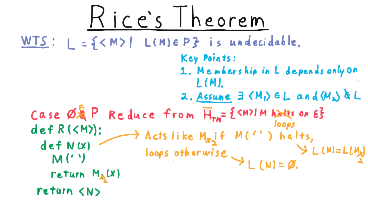
In this case, we just replace \(M_1\) by \(M_2\) in the definition of the reduction, so that \(N\) behaves like \(M_2\) if \(M\) halts on the empty string.
This is fine, but we need to reduce from the complement of \(H_{TM}\): that is, from the set of descriptions of machines that loop on the empty input. Otherwise, we would end up accepting when we wanted to not accept and vice-versa.
All in all then, we have proved the following theorem.

Slightly more intuitively, we can say the following. Let \(L\) be a subset of strings representing Turing machines having two key properties:
- if \(M_1\) and \(M_2\) accept the same set of strings, then their descriptions are either both in or both out of the language–this just says that the language only depends on the behavior of the machine not its implementation.
- the language can’t be trivial–there must be a machine whose description is in the language and a machine whose description is not in the language.
If these two properties hold true, then the language is be undecidable.
Undecidable Properties - (Udacity)
Using Rice’s theorem, we now have a quick way of detecting whether certain questions are decidable. Use your knowledge of the theorem to indicate which of the following properties is decidable. For clarity’s sake, let’s say that a virus is a computer program that modifies the data on the hard disk in some unwanted way.

Conclusion - (Udacity, Youtube)
I want to end this section on computability by revisiting the scene we used at the beginning of the course, where the teacher was explaining functions in terms of ordered pairs, and the students were thinking of what they had to do to x to get y.
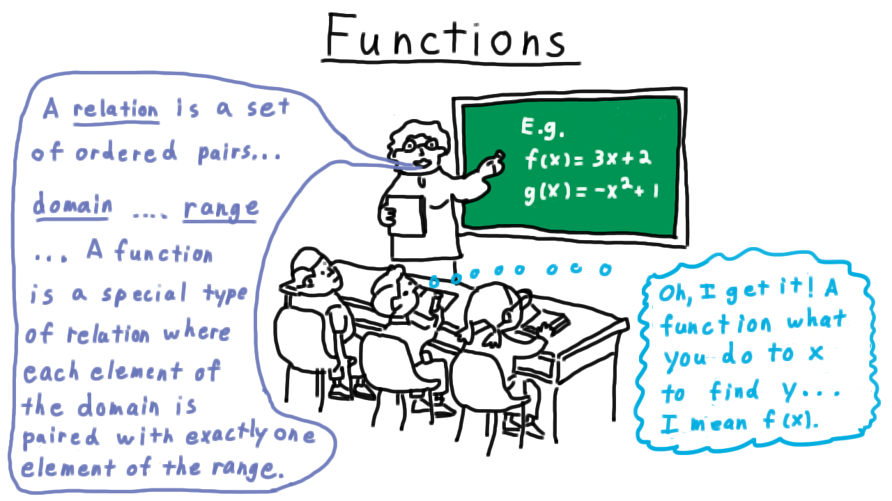
The promise of our study of computability was to better appreciate the difference between these understandings, and I hope you will agree that we have achieved that. We have seen how there are many functions that are not computable in any ordinary sense of the word by a counting argument. We made precise what we meant by computation, going all the way back to Turing’s inspiration from his own experience with pen and paper to formalize the Turing machine. We have seen how this model can compute anything that any computer today or envisioned for tomorrow can. And lastly, we have described a whole family of uncomputable functions through Rice’s theorem.
Towards Complexity - (Udacity, Youtube)
Even since the pioneering work of Turing and his contemporaries such as Alonzo Church and Kurt Godel, mathematical logicians have studied the power of computation and connecting it to provability as well as giving new insights on the nature of information, randomness, even philosophy and economics. Computability has a downside, just because we can solve a problem on a Turing machine doesn’t mean we can solve it quickly. What good is having a computer solve a problem if our sun explodes before we get the answer?
So for now we leave the study of computable functions and languages and move to computational complexity, trying to understand the power of efficient computation and the famous P versus NP problem.
P and NP - (Udacity)
Introduction - (Udacity, Youtube)
So far in the course, we have answered the question: what is computable? We modeled computability by Turing machines and showed that some problems, like the halting problem, cannot be computed at all.
In the next few lectures we ask, what can we compute quickly? Some problems, like adding a bunch of numbers or solving linear equations, we know how to solve quickly on computers. But how about playing the perfect game of chess? We can write a computer program that can search the whole game tree, but that computation won’t finish in our lifetime or even the lifetime of the universe. Unlike computability, we don’t have clean theorems about efficient computation. But we can explore what we probably can’t solve quickly through what known as the P versus NP problem.
P represents the problems we can solve quickly, like your GPS finding a short route to your destination. NP represents problems where we can check that a solution is correct, such as solving a Sudoku puzzle. In this lesson we will learn about P, NP, and their role in helping us understand what we may or may not be able to solve quickly.
Friends or Enemies - (Udacity, Youtube)
We’ll illustrate the distinction between P and NP by trying analyze a world of friends and enemies. Everyone is this world is either a friend or an enemy, and we’ll represent this by drawing an edge between all of the friends like so.
Given all this information, there are several types of analysis that you might want to do, some easier and some harder. For instance, if you wanted to run a dating service, you would be in pretty good shape. Say that you wanted to maximize the number of matches that you make and hence the number of happy customers. Or perhaps, you just want to know if it’s possible to give everyone a date. Well, we have efficient algorithms for finding matchings, and we’ll see some in a future lesson. Here, in this example, it’s possible to match everyone up, and such a matching is fairly easy to find.
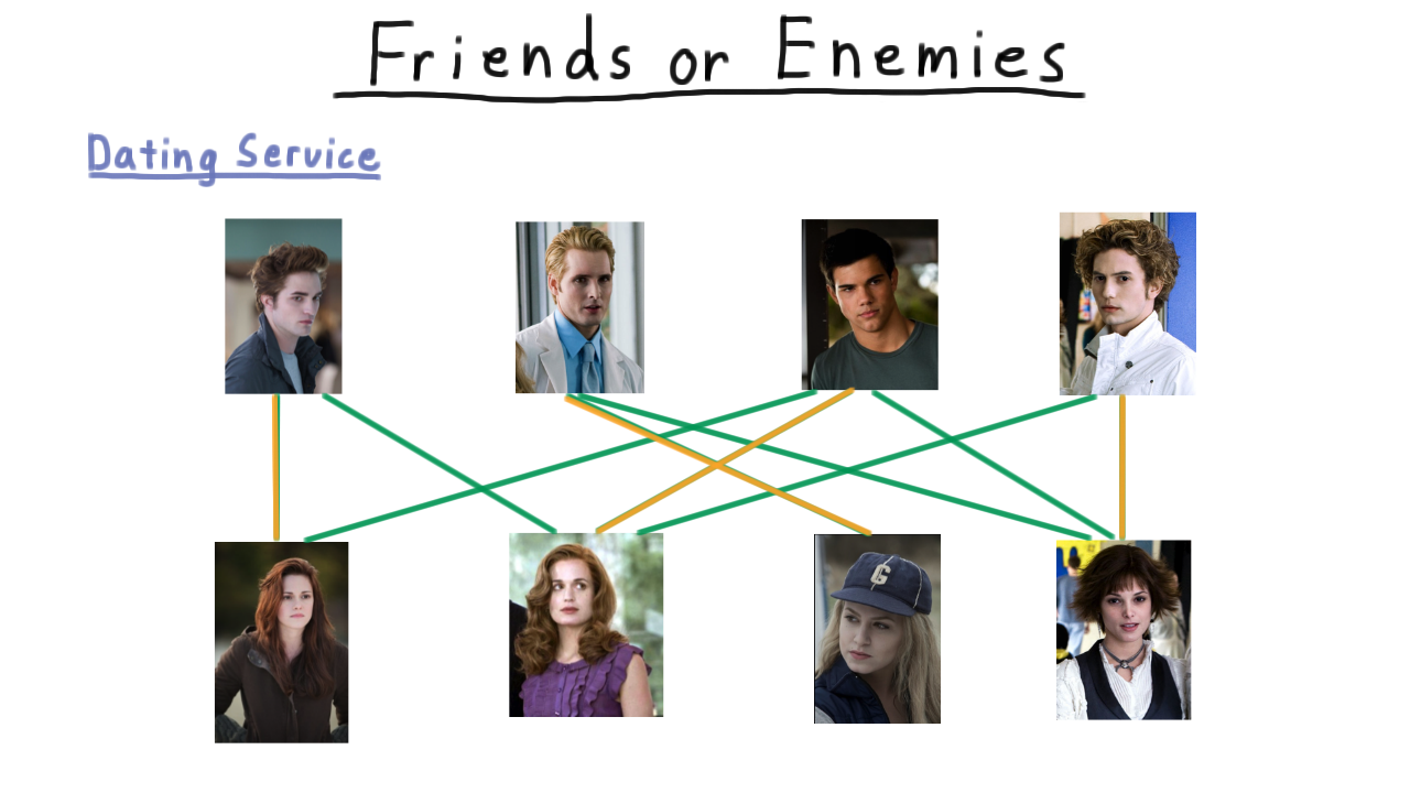
Contrast this with problem of indentifying cliques. By clique, I mean a set of people who are all friends with each other. For instance, here is a clique of size three: every pair of members has an edge between, and cliques of that size aren’t too hard to find.
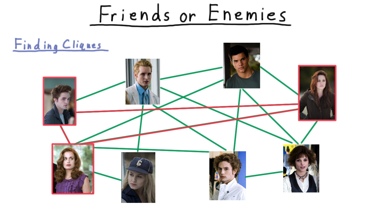
As we start to look for larger cliques, however, the problem becomes harder and harder to solve.
Find a Clique - (Udacity)
In fact, finding a clique of size four, even for a relatively small graph like this one isn’t necessarily easy. See if you can find one.
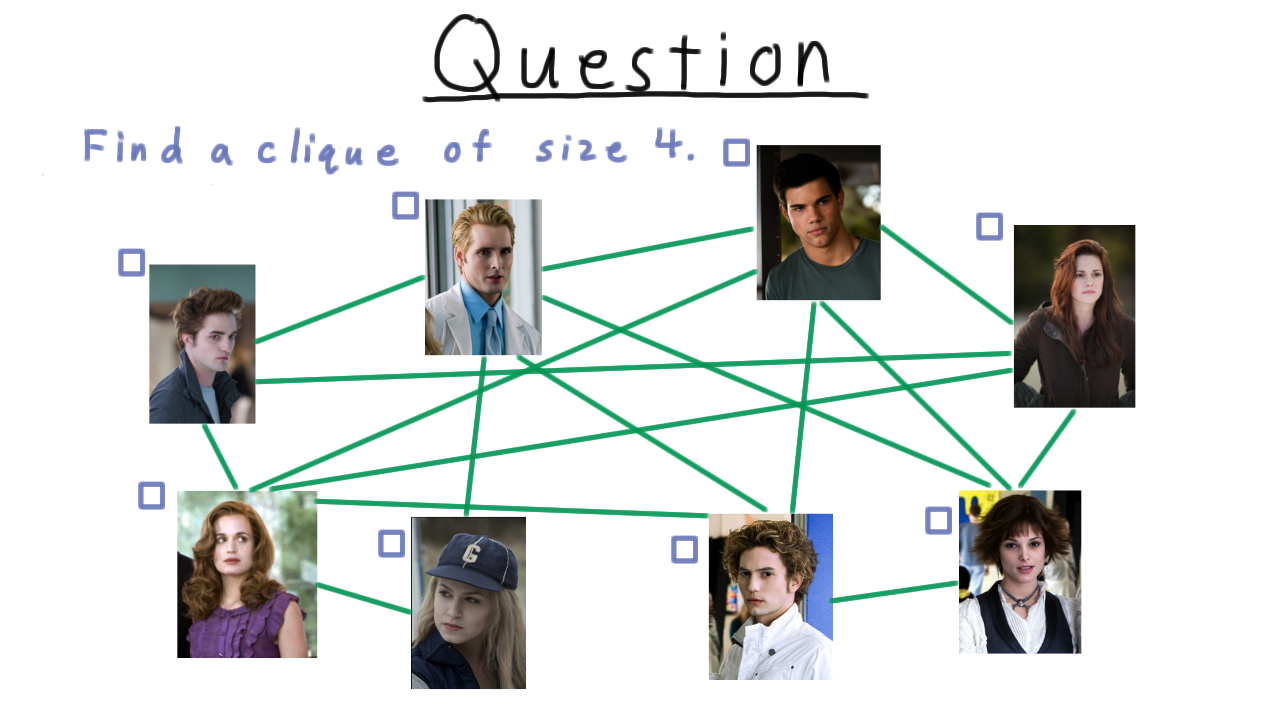
P and NP - (Udacity, Youtube)
Being a little more formal now, we define P to be the set of problems solveable in polynomial time. By polynomial time, we mean that the number of Turing machine steps is bounded a by a polynomial. We’ll formalize this more in a moment. Bipartite matching was one example of this class of problems.
NP we define as the class of problems verifiable in polynomial time. This includes everything in P, since if a problem can be solved in polynomial time, a potential solution can be verified in that time, too. Most computer scientists strongly believe that this containment is strict. That is to say, there are some problems that are efficiently verifiable but not efficiently solvable, but we don’t have a proof for this yet. The clique problem that we encountered is one of the problems that belongs in NP but we think does not belong in P.

There is one more class of problems that we’ll talk about in this section on complexity, and that is the set of NP-complete problems. These are the hardest problems in NP, and we call them the hardest, because any problem in NP can be efficiently transformed into an NP-complete problem. Therefore, if someone were to come up with a polynomial algorithm for even one NP-complete problem, then P would expand out in this diagram, making P and NP into the same class. Finding a polynomial solution for clique would do this, so we say that clique is NP-complete. Since solving problems doesn’t seem to be as easy as checking answers to problems, we are pretty sure that NP-complete problems can’t be solved in polynomial time, and therefore that P does not equal NP.
To computer science novices the difference between matching and clique might not seem to be a big deal and it is surprising that one is so much harder than the other. In fact, the difference between a polynomially solvable problem and a NP-complete one can be very subtle. Being able to tell the difference is an important skill for anyone who will be designing algorithms for the real world.
Delicacy of Tractability - (Udacity, Youtube)
As we discussed, one way to see the sublety of the difference between problems in P and those that are NP-complete is to compare what it takes to solve seemingly similar real-world problems.
Consider the shortest path problem. You are given two locations and you want to find the shortest valid route between them. You phone does this in a matter of milliseconds when you ask it for directions, and it gives you an exact answer according to whatever model for distance it is using. This is computationally tractable.
On the other hand, consider this warehouse scenario where a customer places an order for several different items and a person or a robot has to go around and collect them before going to the shipping area for them to be packed. This is called the traveling salesman problem and it is NP-complete. This problem also comes up in the unofficial guide to Disneyworld, which tries to tell you how to get to all the rides as quickly as possible.
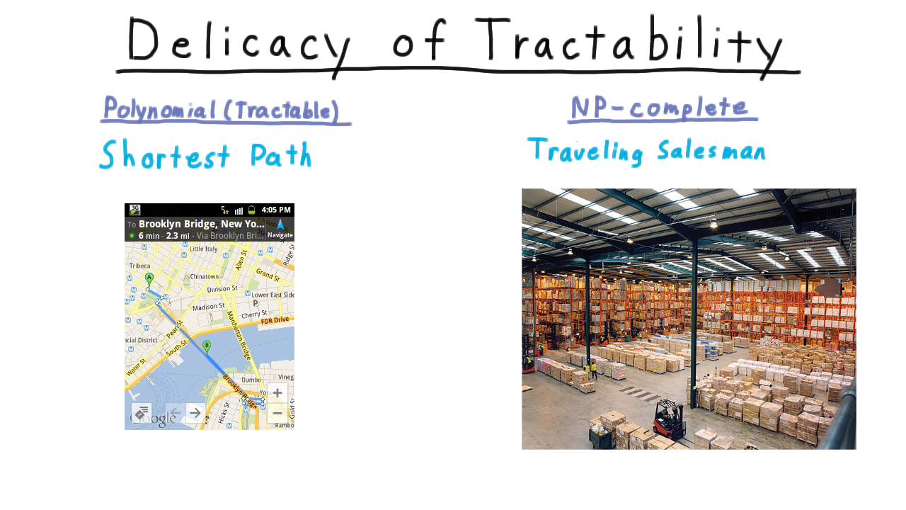
This explains why your phone can give you directions but supply chain logistics–just figuring out how things should be routed– is a billion dollar industry.
Actually, however, we don’t even need to change the shortest path so much to get an NP-complete problem. Instead of asking for the shortest path, we could ask for the longest, simple path. We have to say simple so that we don’t just go around in cycles forever.
This isn’t the only possible pairing of similar P and NP-complete problems either. I’m going to list some more. If you aren’t familiar with these problems yet, don’t worry. You will learn about them by the end of the course. Vertex cover in bipartite graphs in polynomial, but vertex cover in general graphs is NP complete.
A class of optimization problems called Linear Programming is in P, but if we restrict the solutions to integers, then we get an NP-complete problem Finding an Eulerian cycle in a graph where you touch each edge once is polynomial. On the other hand, finding a Hamiltonian cycle that touches each vertex once is NP-complete
And lastly, figuring out whether a boolean formula with two literals per clause is polynomial, but if there are three literals per clause, then the problem is NP-complete.

Unless you are familiar with some complexity theory, problems in P aren’t always easy to tell from those that are NP-complete. Yet, in the real world when you encounter a problem it is very important to know which sort of problem you are dealing with. If your problem is like one of the problems in P, then you know that there should be an efficient solution and you can avail yourself of the wisdom of many other scientists who have thought hard about how to efficiently solve these problems. On the other hand, if your problem is like one the NP-complete problems, then some caution is in order. You can expect to be able to find exact solutions for small enough instances, and you may be able to find a polynomial algorithm that will give an approximate solution that is good enough, but you should not expect to find an exact solution that will scale well for all cases.
Being able to know which situation you are in is one of the main practical benefits of studying complexity.
Running Time Analysis - (Udacity, Youtube)
Now, we are going to drill down into the details and make many of the notions we’ve been talking about more precise. First we need to define running time.
We’ll let M be a Turing machine– single-tape, multi-tape, random access, the definition works for all of them. The running time of the machine then is a function over the natural numbers where f(n) is the largest number of steps taken by the machine for an input string of length n. We can extend this definition to machines that don’t halt as well by making their running time infinite. We always consider the worst case.
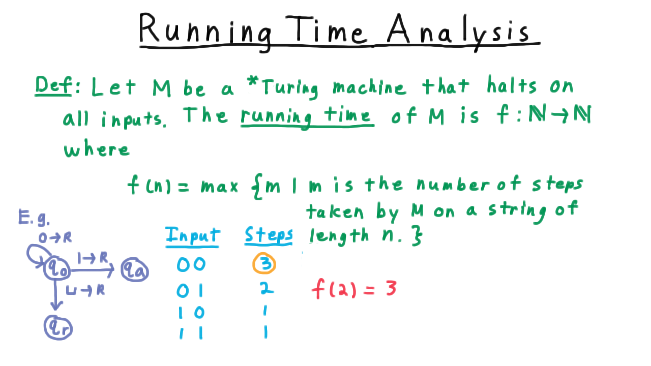
Let’s illustrate this idea with an example. Consider the single-tape machine in the figure above that takes binary input and tests whether the input contains a 1. Let’s figure out the running time for string of length 2. We need to consider all the possible strings of length 2, so we make a table and count the number of steps. The largest number of steps in 3, where we read both zeros and then the blank symbol. Therefore, f(2) = 3.
Asymptotic Analysis - (Udacity, Youtube)
Now, it’s not very practical to write down every running time function exactly, so computer scientists use various levels of approximation. For complexity, we use asymptotic analysis. We’ll do a very brief review here, but if you haven’t seen this idea before you should take a few minutes to study it on your own before proceeding with the lesson.
In words, the set \(O(f(n))\) is the set of functions \(g\) such that \(g \leq cf(n)\) for sufficiently large \(n\). Making this notion of “sufficiently large \(n\)” precise, we end up with
Even though we’ve defined \(O(f(n))\) as a set, we write \(g(n) = O(f(n))\) instead of using the inclusion sign. We also say that \(g\) is order \(f\).
This definition can be a little confusing, but it should feel like the definition of a limit from your calculus class. In fact, we can restate this condition to say that the ratio of \(g\) over \(f\) converges to a constant under the limsup.
An example also helps. Take the function \(g(n) = n^2 - n + 10.\)
We can argue that this is order \(n^2\) by choosing \(c = 1\) and \(N = 10\). For every \(n \geq 10\) , \(n^2\) is greater than the function \(g\).
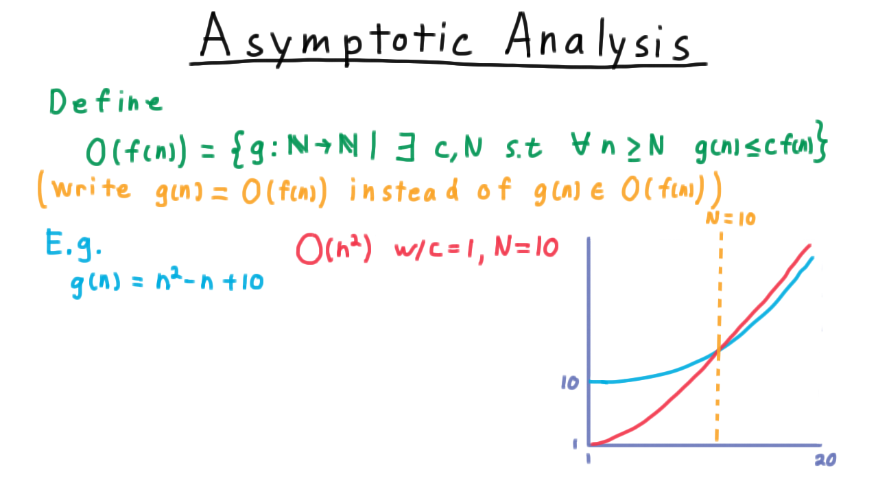
We also could have chosen \(c = 10\) and \(N = 1.\)
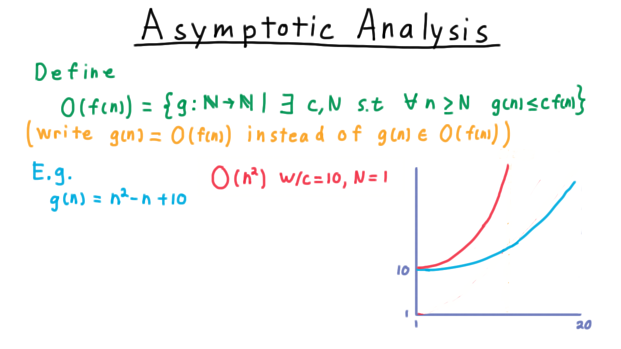
Note that the big-O notation does not have to create a tight bound. Thus, \(g = O(n^3)\) too. Setting \(c= 1\) and \(N= 3\) works for this.
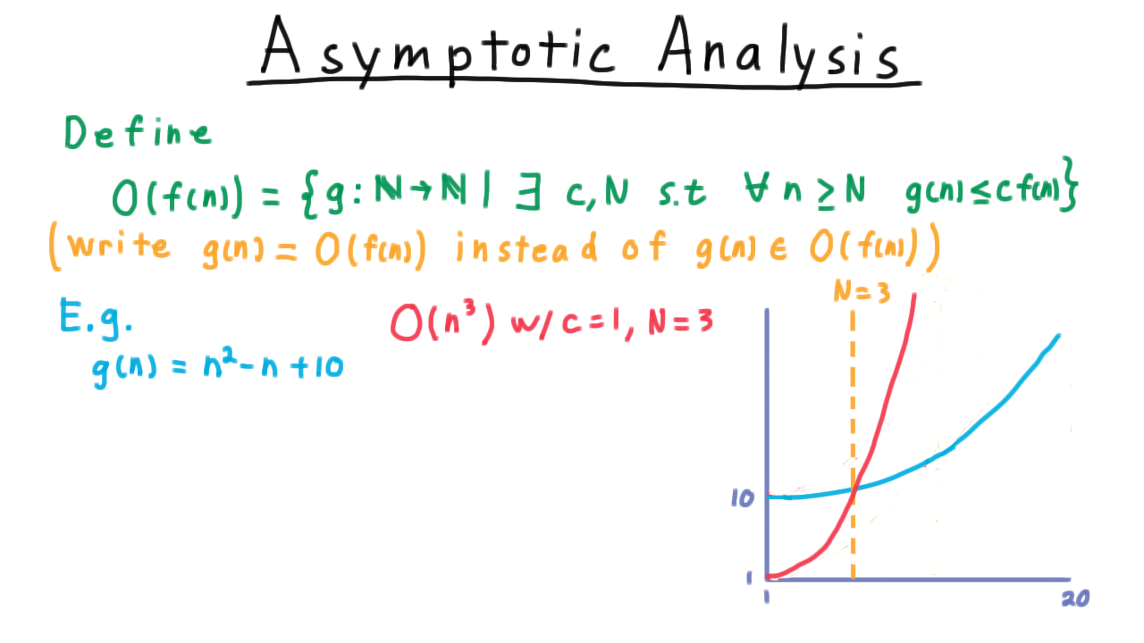
Big O Question - (Udacity)
Once we’ve established the running time for an algorithm, we can analyze other algorithms that use it as a subroutine much more easily. Consider this question. Suppose that algorithm A has running time O(n), and A is called by algorithm B O(log n) times, and algorithm B runs for an additional log-squared n time afterwards. What is the tightest bound on the running time of B?
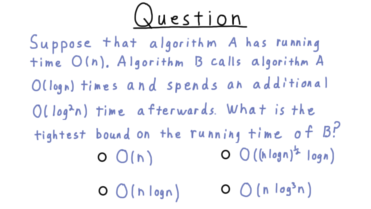
The Class P - (Udacity, Youtube)
We are now ready to formally define the class P. Most precisely,
P is the set of languages recognized by an order \(n^k\) deterministic Turing machine for some natural number \(k\).
There are several important things to note about this definition.
- First is that P is a set of languages. Intuitively, we talk about it as a set of problems, but to be rigorous we have to ultimately define it in terms of languages.
- Second is the word deterministic. We haven’t seen a non-deterministic Turing machine yet, but one is coming. Deterministic just means that given a current state and tape symbol being read, there is only one transition for the machine to follow.
- An \(n^k\) time machine here is one with running time order \(n^k\) as we defined these terms a few minutes ago.

Perhaps the most interesting thing about this definition is the choice for any \(k\) in the natural numbers. Why is this the right definition? After all, if \(k\) is 100 then deciding the language isn’t tractable in practice.
The answer is that P doesn’t exactly capture what is tractable in practice. It’s not clear that any mathematical definition would stand the test of time in this regard, given how often computers change, or be relevant in so many contexts. This choice does have some very nice properties however.
- It matches tractability better than one might think. In practice, k is usually low for polynomial algorithms, and there are plenty of interesting problems not known to be in P.
- The definition is robust to changes to the model. That is to say, P is the same for single-tape, multi-tape machines, Random Access machines and so forth. In fact, we pointed out that the running times for each of those models are polynomially related when we introduced them.
- P has the nice property of closure under the composition of algorithms. If one algorithm calls another algorithm as a subroutine a polynomial number of times, then that algorithm is still polynomial, and the problem it solves is in P. In other words, if we do something efficient a reasonably small number of times, then the overall solution will be efficient. P is exactly the smallest class of problems containing linear time algorithms and which is closed under composition.
Problems and Encodings - (Udacity, Youtube)
We’ve defined P as a set languages, but ultimately, we want to talk about it as a set of problems. Unfortunately, this isn’t as easy as it might seem. The encoding rules we use for turning abstract problems into strings can affect whether the language is in P or not. Let’s see how this might happen.
Consider the question: Does G have a Hamiltonian cycle–a cycle that visits all of the vertices? Here is a graph and here is its adjacency matrix.

A natural way to represent the graph as a string is to write out its adjacency matrix in scanline order as done in the figure above. But this isn’t the only way to encode the graph. We might do something rather inefficient.
The scanline encoding for this graph represents the number 170 in binary. We could choose to represent the graph in essentially unary.
We might represent the graph as 342 zeros followed by 170 ones. The fact that there are 29=512 symbols total indicates that it’s a 3x3 matrix, and converting 170 back into binary gives us the entries of the adjacency matrix.

This is a very silly encoding, but there is nothing invalid about it.
This language, it turns out, is in P, not because it allows the algorithm to exploit any extra information or anything like that, but just because the input is so long. The more sensible, concise encoding isn’t known to be in P (and probably isn’t, by an overwhelming consensus of complexity theorists). Thus, a change in encoding can affect whether a problem is in P, yet it’s ultimately problems that we are interested in, independent of the particulars of the encoding.
We deal with this problem, essentially by ignoring unreasonable representations like this one. As long as we consider any reasonable encoding (think about what xml or json would produce from how you would store it in computer memory) then the particulars won’t change the membership of the language in P, and hence we can talk at least informally about problems being in P or not.
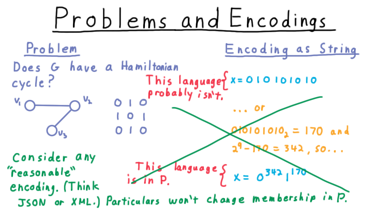
Which are in P - (Udacity)
Now that we have defined P, I want to illustrate how easy it can be to recognize that a problem is in P. Recognizing that a problem is NOT in P is a little harder, so for this exercise assume that if the brute-force algorithm is exponential, so is the best algorithm. Consider a finite set U of the integers and the following three problems. Check the ones that you think are in P. (Again, if there isn’t an obvious polynomial-time algorithm, assume that there isn’t one.)
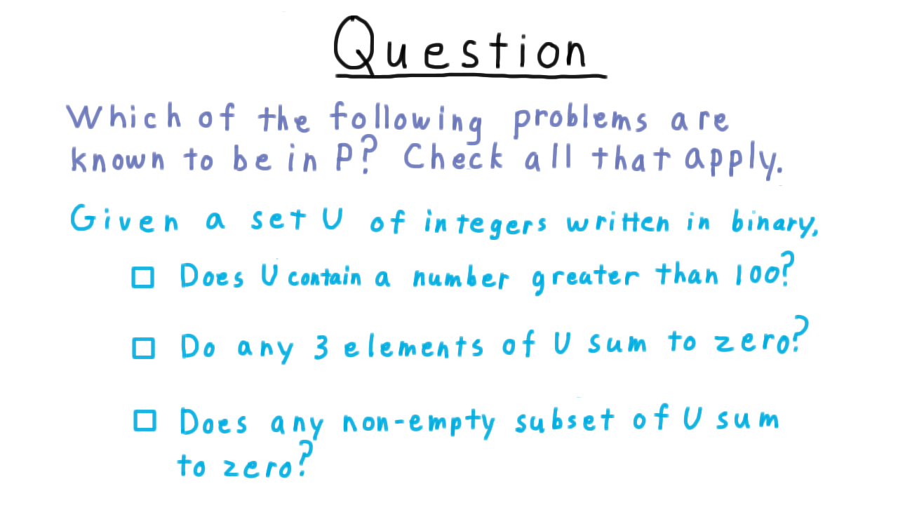
Nondeterministic TMs - (Udacity, Youtube)
From the class P, we now turn to the class NP. At the beginning of the lesson, I said that NP is the class of problems verifiable in polynomial time. This is true, but it’s not how we typically define it. Instead, we define NP as the class of problems solvable in polynomial time on a nondeterministic Turing machine, a variant that we haven’t encountered before.
Nondeterminism in computer science is often misunderstood, so put aside whatever associations you might have had with the word. Perhaps the best way to understand nondeterministc Turing machines is by contrasting a nondeterministic computation with a deterministic one. A deterministic computation starts in some initial state and then the next state is exactly uniquely determined by the transition function. There is only one possible successor configuration.
And to that configuration there is only one possible successor.
And so on and so forth. Until an accepting or rejecting configuration is reached, if one is reached at all.

On the other hand, in a nondeterministic computation, we start in a single initial configuration, but it’s possible for there to be multiple successor configurations. In effect, the machine is able to explore multiple possibilities at once. This potential splitting continues at every step. Sometimes there might just be one possible successor state, sometimes there might be three or more. For each branch, we have all the same possibilities as for a deterministic machine.
- It can reject.
- It can loop forever.
- It can accept.
If the machine ever accepts in any of the these branches, then the whole machine accepts.
The only change we need to make to the 7-tuple of the deterministic Turing machine needed to make it nondeterministic is to modify the transition function. An element of the range is no longer the set of single (state, tape-symbol to write, direction to move) tuple, but a collection of all such possibilities.
\[ \delta: Q \times \Gamma \rightarrow \{S \; | \; S \subseteq Q \times \Gamma \times \{L,R\} \} \]
This set of all subsets used in the range here is often called a power set.
The only other change that needs to be made is when the machine accepts. It accepts if there is any valid sequence of configurations that results in an accepting state. Naturally, then it also rejects only when every branch reaches a reject state. If there is a branch that hasn’t rejected yet, then we need to keep computing in case it accepts.
Therefore, a nondeterministic machine that never accepts and that loops on at least one branch will loop.
Which Language - (Udacity)
Here is the state transition diagram for a simple nondeterministic Turing machine. The machine starts out in \(q_0\) and then it can move the head to right on 0s and 1s, OR on a 1, it can transition to state \(q_1.\)
The fact that there are two transitions out of state \(q_0\) when reading a 1 is the nondeterministic part of the machine. In branches where the transition to state \(q_1\) is followed, the Turing machine reads one more 0 or 1 and then expects to hit the end of the input. Remember that by convention, if there is no transition specified in one of these state diagrams, then the machine simply moves to the reject state and halts. That keeps the diagrams from getting cluttered.
My question to you then is what language does this machine recognize? Check the appropriate answer.
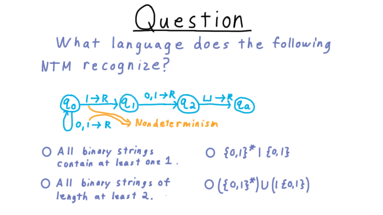
Composite Numbers - (Udacity, Youtube)
To get more intuition for the power of nondeterminism, let’s see how much more efficient it makes deciding the language of composite numbers–that is, numbers that are not prime. The task is to decide the string representations of numbers that are the product of two positive integers, greater than 1.
One deterministic solution looks like this.

Think of the flow diagram as capturing various modules within the deterministic Turing machine. We start by initializing some number \(p\) to 1. Then we increment it, and test whether p-squared is greater than \(x\). If it is, then trying larger values of p won’t help us, and we can reject. If p-squared is no larger than \(x\), however, then we test to see if p divides x. If it does, we accept. If not, the we go try the next value for \(p.\)
Each iteration of this loop require a number of steps that is polynomial in the number of bits used to represent x. The trouble is that we might end up needing \(\sqrt{x}\) iterations of this outer loop here in order to find the right p or confirm that one doesn’t exist. This what makes the deterministic algorithm slow. Since the value of x is exponential in its input size–remember that it is represented in binary–this deterministic algorithm is exponential.
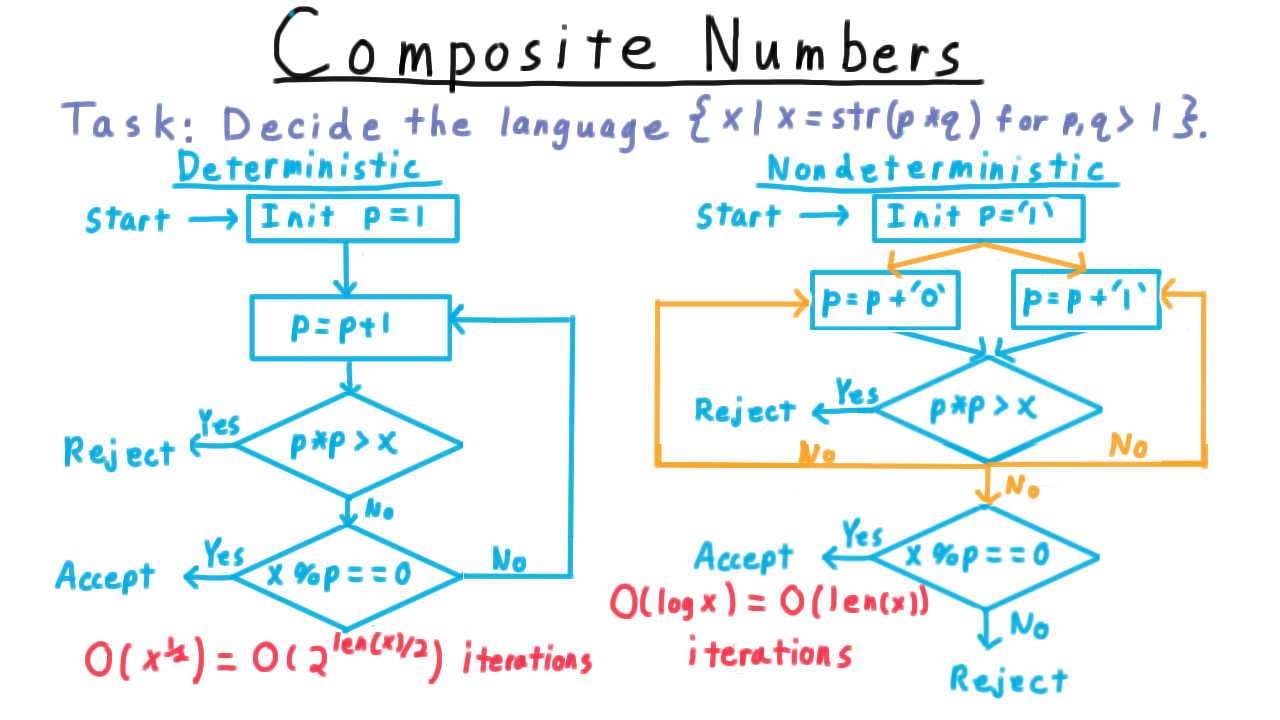
On the other hand, with nondeterminism we can do much better. We initalize p so that it is represented on it’s own tape as the number 1 written in binary. Then we nondeterministically modify \(p.\) By having two possible transitions for the same state and symbol pair, we can non-deterministically append a bit to p. (The non-deterministic transitions are in orange.)
Next, we check to see if we have made \(p\) too large. If we did, then there is no point in continuing, so we reject.
On the other hand, if \(p\) is not too big, then we nondeterministically decide either to
- append a zero to \(p\),
- append a 1 to \(p\), or
- leave \(p\) as it is and go see if it divides \(x.\)
If there is some p that divides \(x\), then some branch of the computation will set \(p\) accordingly. That branch will accept and so the whole machine will. On the other hand, if no such \(p\) exists, then no branch will accept and the machine won’t either. In fact, the machine will always reject because every branch of computation will be rejected in one of the two possible places.
This non-deterministic strategy is faster because it only requires \(\log x\) iterations of this outer loop. The divisor \(p\) is set one bit at a time and can’t use more bits than \(x,\) the number it’s supposed to divide.
Thus, while the deterministic algorithm we came up with was exponential in the input length, it was fairly easy to come up with a nondeterminstic one that was polynomial.
The Class NP - (Udacity, Youtube)
We are almost ready to define the class NP. First, however, we need to define running time for a nondeterministic machine, because it operates differently from a deterministic one.
Since we think about all of these possible computations running in parallel, the running time for each computational path is the path length from the initial configuration.
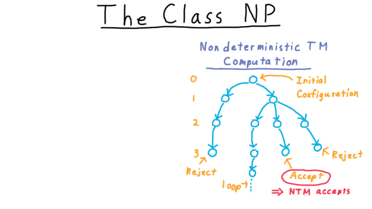
And the running time of the machine as a whole is the maximum number of steps used on any branch of the computation. Note that once we have a bound the length of any accepting configuration sequence, we can avoid looping by just creating a timeout.
NP is the set of languages recognized by an \(O(n^k)\) time nondeterministic Turing machine for some number \(k.\)
In other words, it’s the set of languages recognized in polynomial time by a nondeterministic machine. NP stands for nondeterministic polynomial time.
Nondeterminism can be a little confusing, but it helps to remember that a string is recognized if it leads to any accepting computation–i.e. any accepting path in this tree. Note that any Turing machine that is a polynomial recognizer for a language can easily be turned into a polynomial decider by adding a timeout since all accepting computations are bounded in length by a polynomial.
NP Equals Verifiability Intuition - (Udacity, Youtube)
At the beginning of the lesson, we identified NP as those problems for which answer can be verified in polynomial time. Remember how easy it was to check that a clique was a clique? In the more formal treatment, however, we defined NP as those langauges recognized by nondeterministic machines in polynomial time. Now we get to see why these mean the same thing.
To get some intuition, we’ll revisit the example of finding a clique of size 4. We already discussed how a clique of size 4 is easy to verify, but how is it easy to find it with a non-deterministic machine? The key is to use the non-determinism to create a branch of computation for each subset of size 4, and then use our verification strategy to decide whether any of those subsets corresponds to a clique.
Remember that if any sequence of configurations accepts, then the non-deterministic machine accepts.
One branch of computation might choose these 4 and then reject because it’s not a clique.
Another branch might choose these 4 and also reject.
But one branch will choose the correct subset and this will accept.
And, that’s all we need. If one branch accepts then the whole non-deterministic machines does, as it should. There is a clique of size 4 here.
NP Equals Verifiability - (Udacity, Youtube)
Now for the more formal argument.
A verifier for a language \(L\) is a deterministic Turing machine \(V\) such that \(L\) is equal to the set of strings \(w\) for which there is another string \(c\) such that \(V\) accepts the pair \((w,c).\)
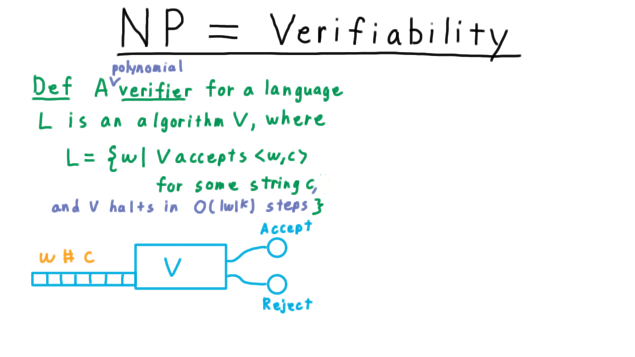
In other words, for every string \(w \in L\), there is a “certificate” c that can be paired with it so that V will accept, and for every string not in \(L\), there is no such string \(c\). It’s intuitive to think of \(w\) as a statement and of \(c\) as the proof. If the statement is true, then there should be a proof for it that \(V\) can check. On the other hand, if \(w\) is false, then no proof should be able to convince the verifier that it is true.
A verifier is polynomial if it’s running time is bounded by a polynomial in \(w.\)
Note that this \(w\) is the same one as in the definition. It is the string that is a candidate for the language. If we included the certificate \(c\) in the bound, then it becomes meaningless since we could make \(c\) be as long as necessary. That’s a polynomial verifier.
We claim
The set of Languages that have polynomial time verifiers is the same as NP.
The key to understanding this connection is once again this picture of the tree of computation performed by the nondeterministic machine.
If a language is in NP, then there is some nondeterministic machine that recognizes it, meaning that for every string in the language there is an accepting computation path. The verifier can’t simulate the whole tree of the nondeterministic machine in polynomial time, but it can simulate a single path. It just needs to know which path to simulate.
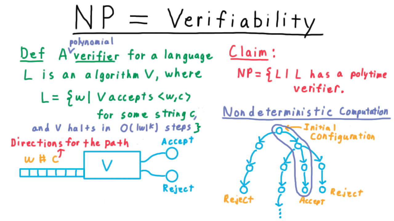
But this is what the certificate can tell it. The certificate can act as directions for which turns to make in order to find the accepting computation of the nondeterministic machine. Hence, if there is nondeterministic machine that can recognize a language, then there is a verifier that can verify it.
Now, we’ll argue the other direction. Suppose that V verifies a language. Then, we can build a nondeterministic machine whose computation tree will look a bit like a jellyfish. It the very top, we have a high degree of branching as the machine nondeterministically appends a certificate c to its input.
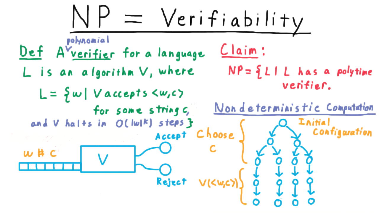
Then it just deterministically simulates the verifier. If there is any certificate that causes V to accept, the nondeterministic machine will find it. If there isn’t one, then the nondeterministic machine won’t.
Which is in NP - (Udacity)
Now that we’ve defined NP and defined what it means to be verifiable in polynomial time, I want you to apply this knowledge to decide if several problems are in NP. First, is a graph connected? Second, does a graph have a set of k vertices with no edges between? This is called the independent set problem. And lastly, will a given Turing machine M accept exactly one string?
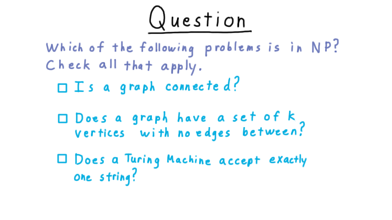
Conclusion - (Udacity, Youtube)
In this lesson, we have introduced the P and NP classes of problems. As we said in the beginning, the class P informally captures the problems we can solve efficiently on a computer, and the class NP captures those problems whose answer we can verify efficiently on a computer. Our experience with finding a clique in a graph suggests that these two classes are not the same. Cliques are hard to find but they are easy to check. And it is simply intuitive that solving a difficult problem should be harder than just checking a solution.
Nevertheless, no one has been able to prove that P is not equal to NP. Whether these two classes are equivalent is the known as the P versus NP question, and it is the most important open problem in theoretical computer science today if not in all of mathematics. We’ll discuss the full implications of the question in a later lecture, but for now, I’ll just mention that in the year 2000, the Clay Math Institute named the P versus NP problem as one of the seven most important open questions in mathematics and has offered a million-dollar bounty for a proof that determines whether or not P = NP. Fame and fortune await the person who settles the P v NP problem, but many have tried and failed.
Next class we look at the NP-complete problems, the hardest problems in NP.
NP-Completeness - (Udacity)
Introduction - (Udacity, Youtube)
This lecture covers the theory of NP-completeness, the idea that there are some problems in NP so general and so expressive that they capture all of the challenges of solving any problem in NP in polynomial time. These problems provide important insight into the structure of P and NP, and form the basis for the best arguments we have for the intractability of many important real-world problems.
The Hardest Problems in NP - (Udacity, Youtube)
With our previous discussion of the classes P and NP in mind, you can visualize the classes P and NP like this.
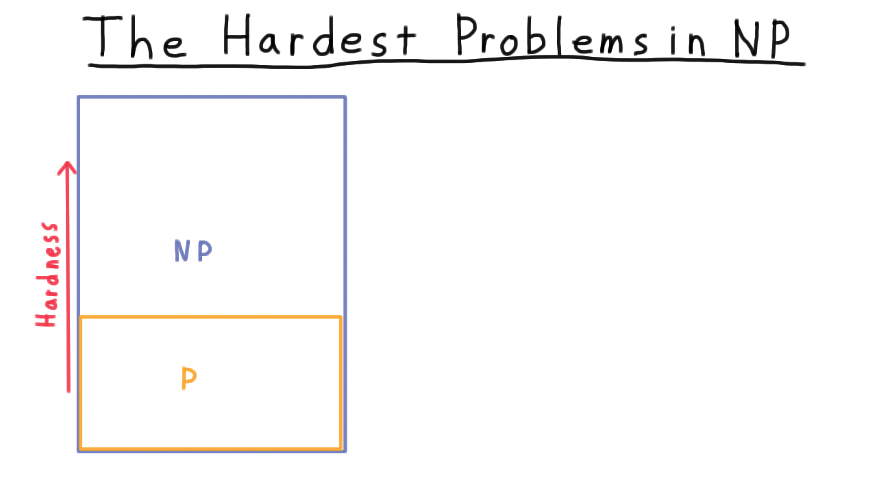
Clearly, P is contained inside of NP, and we are pretty sure that this containment is strict. That is to say that there are some problems in NP but not in P, where the answer can be verified efficiently, but it can’t be found efficiently. In this picture then, you can imagine the harder problems being at the top.
Now, suppose that you encounter some problem where you know how to verify the answer, but where you think that finding an answer is intractable. Unfortunately, your boss or maybe your advisor doesn’t agree with you and keeps asking for an efficient solution.
How would you go about showing that the problem is in fact intractable? One idea is to show that the problem is not in P. That would indeed show that it is not tractable, but it would do much more. It would show that P is not equal to NP. You would be famous. As we talked about in the last lecture, whether P is equal to NP is one of the great open questions in mathematics. Let’s rule option out. I don’t want to discourage you from trying to prove this theorem necessarily. You just should know what you are getting into.
Another possible solution is to show that if you could solve your problem efficiently then it would be possible to solve another problem efficiently, one that is generally considered to be hard. If you were working in the 1970’s you might have shown that a polynomial solution to your problem would have yielded a polynomial solution to linear programming. Therefore, your problem must be at least as hard a linear programming. The trouble with this approach is that it was later shown that linear programming actually was polynomially solvable. Hence, the fact your problem is as hard as linear programming doesn’t mean much anymore. The class P swallowed linear programming. Why couldn’t it swallow your program as well? This type of argument isn’t worthless, but it’s not as convincing as it might be.
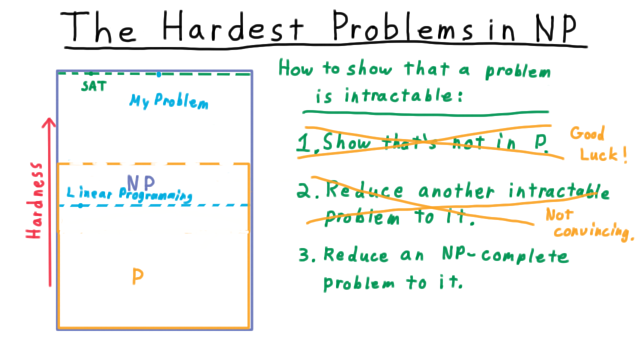
It would be much better to reduce your problem to a problem that we knew was one of the hardest in the class NP, so hard that if the class P were to swallow it would have to have swallowed all of NP. In other words, we would have to move the P borderline all the way to the top. Such a problem would have to be NP-complete, meaning that we can reduce every language in NP to it. Remarkable as it may seem, it turns out that there are lots of such languages–satisfiability being the first for which this was proved. In other words, we know that it has to be at the top of this image. Turning back to how to show that your problem is intractable, short of proving that P is not equal to NP, the best we can do is to reduce an NP-complete problem like SAT to your problem. Then, your problem would be NP-Complete too, and the only way your problem could be polynomially solvable is if everything in NP is.
There are two parts to this argument.
- The first is the idea of a reduction. We’ve seen reductions before in the context of computability. Here the reductions will not only have to be computable but computable in polynomial time. This idea will occupy the first half of the lesson.
- The second half will consider this idea of NP-completeness and we will go over the famous Cook-Levin theorem which show that boolean satisfiability is NP-complete
Polynomial Reductions - (Udacity, Youtube)
Now for the formal definition of a polynomial reduction. This should feel very similar to the reductions that we considered when were talking about computability.
A language \(A\) is polynomially reducible to language \(B\) (\(A \leq_P B\)) if there is a polynomial-time computable function \(f\) where for every string w,
\[w \in A \Longleftrightarrow f(w) \in B.\]
The key difference from before is that we have now required that the function be computable in polynomial time, not just that it be computable. We will also say that \(f\) is a polynomial time reduction of \(A\) to \(B.\)
Here is key implication of there being a polynomial reduction of one language to another. Let’s suppose that I want to be able to know whether a string \(x\) is in the language \(A\), and suppose also that there exists a polynomial time decider \(M\) for the language \(B.\)
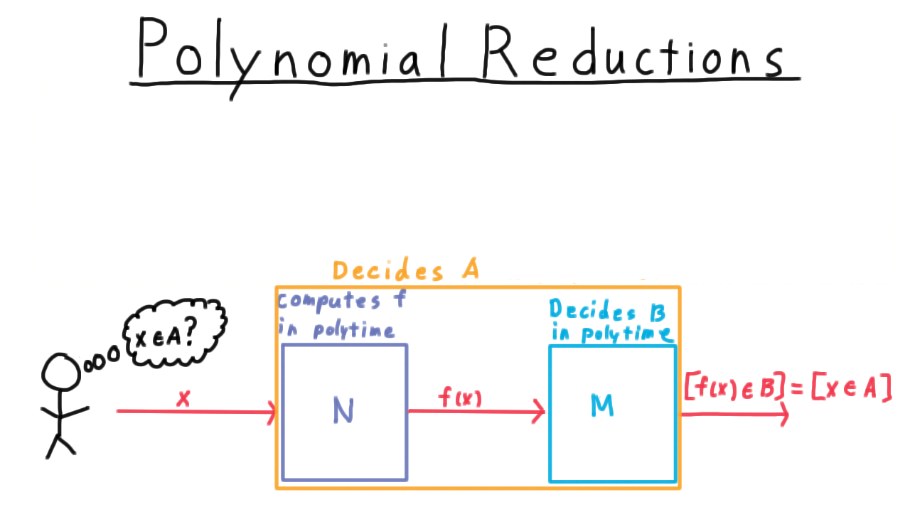
Then, all I need to do is take the machine or program that computes this function–let’s call it \(N\)–
and feed my string \(x\) into it, and then feed that output into \(M.\) The machine \(M\) will tell me if \(f(x)\) is in \(B.\) By the definition of a reduction, this also tells me whether \(x\) is in \(A,\) which is exactly what I wanted to know. I just had to change my problem into one encoded by the language \(B\) and then I could use \(B\)’s decider.
Therefore, the composition of \(M\) with \(N\) is a decider for \(A\) by all the same arguments we used in the context of computability. But is it a polynomial decider?
Running Time of Composition - (Udacity)
We just found ourselves considering the running time of the composition of two Turing machines. Think carefully, and give the most appropriate bound for the running time of the composition of \(M\) which runs in time \(q\) with \(N\) which runs in time \(p.\) You can assume that both \(N\) and \(M\) at least read all of their input.
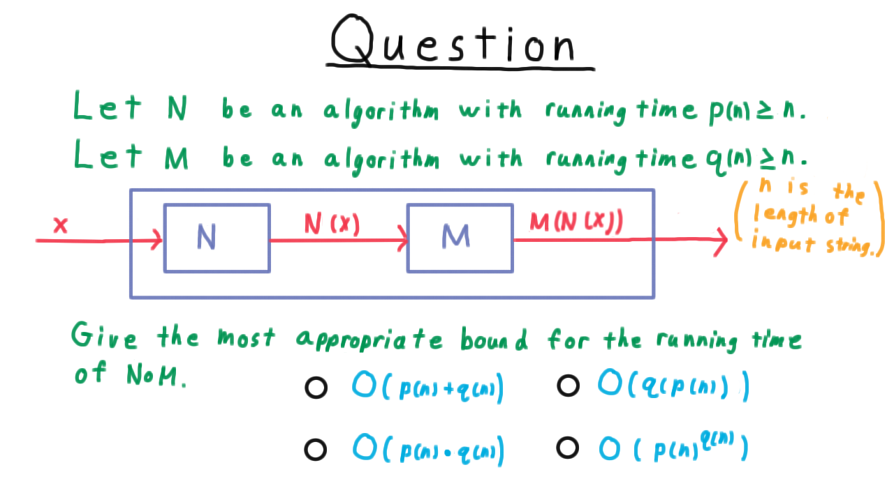
Polynomial Reductions Part 2 - (Udacity, Youtube)
We just argued that if \(N\) is polynomial and we take its output and feed that into \(M\) which is also polynomial in its input size, then the resulting composition of \(M\) with \(N\) is also polynomial. Therefore, we can add “in polytime” to our claim in the figure.

By this argument, we’ve proved the following important theorem.
If A is polynomially reducible to B, and B is in P, then A must be in P.
Just convert the input string to prepare it for the decider for \(B,\) and return what the decider for \(B\) says.
What Do Reductions Imply - (Udacity)
Here is a question to test your understanding of the implications of the existence of a polynomial reduction. Suppose that \(A\) reduces to \(B,\) which of the statements below follow?
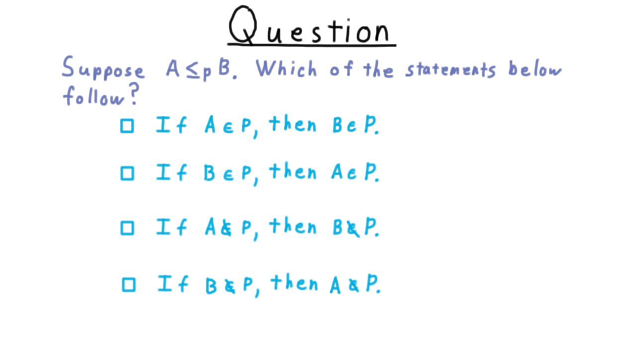
Independent Set - (Udacity, Youtube)
To illustrate the idea of a polynomial reduction, we’re going to reduce the problem of finding a Independent Set in a graph to that of finding a Vertex Cover. In the next lesson, we going to argue that if P is not equal to NP, then Indepedent Set is not in P, so Vertex Cover can’t be either. But that’s getting ahead of ourselves. For the benefit of those not already familiar with these problems, we will state them briefly.
First, we’ll consider the independent set problem and see how it is equivalent to the Clique problem that we talked about when we introduced the class NP.
Given a graph, a subset \(S\) of the vertices is an independent set if there are no edges between vertices in \(S.\)
These two vertices here do not form an independent set because there is an edge between them.

However, these three vertices do form an independent set because there are no edges between them.
Clearly, each individual vertex forms an independent set, since there isn’t another vertex in the set for it to have an edge with, and the more vertices we add the harder it is to find new ones to add. Finding a maximum independent set, therefore, is the interesting question. Phrased as a decision problem, the question becomes “given a graph G, is there an independent set of size \(k\)?”
Find an Independent Set - (Udacity)
In order to understand the reduction, it is critical that you understand the independent set problem, so here is a quick question to test your understanding. Mark an independent set of size 3.
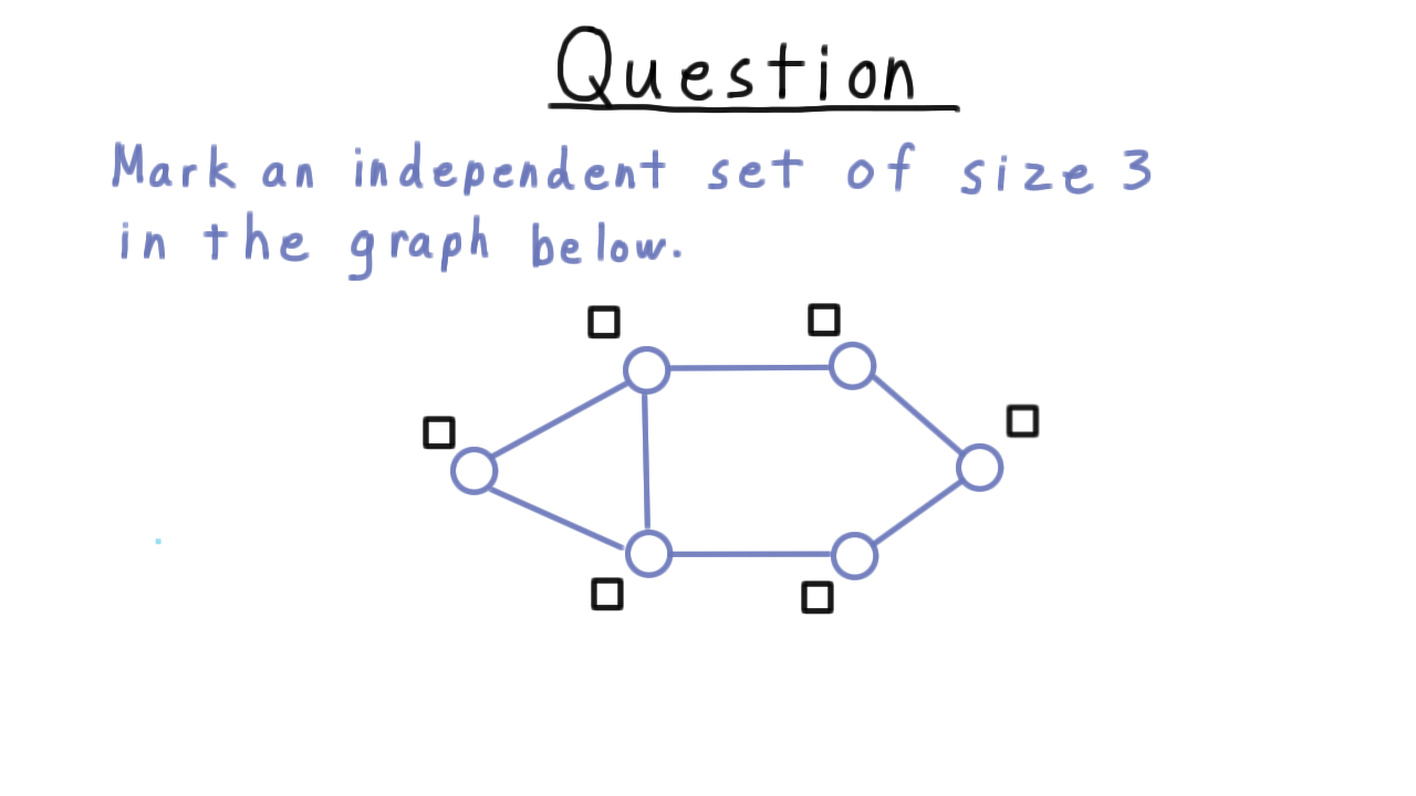
Vertex Cover - (Udacity, Youtube)
Now let’s define the other problem that will be part of our example reduction, Vertex Cover.
Given a graph G, a subset \(S\) of the vertices forms a vertex cover if every edge is indicident on \(S\) (i.e. has one part in \(S\)).
To illustrate, consider this graph here. These three shaded vertices do not form a vertex cover.
On the other hand, the two vertices do form a vertex cover because every edge is incident on one of these two.
Clearly, the set of all vertices is a vertex cover, so the interesting question is how small a vertex cover can we get. Phrased as a decision questionwhere we are give a graph G, it becomes “Is there a vertex cover of size \(k\)?”
Note that this problem is in NP. It’s easy enough to check whether a subset of vertices is of size \(k\) and whether it covers all the edges.
Find a Vertex Cover - (Udacity)
Going forward, it will be very important to understand this vertex cover problem, so we’ll do a quick exercise to give you a chance to test your understanding. Mark a vertex cover of size 3 in the graph below.

Vertex Cover = Ind Set - (Udacity, Youtube)
Having defined the Independent Set and Vertex Cover problems, we will now show that Vertex Cover is as hard as Independent set. In general, finding a reduction can be very difficult. Sometimes, however, it can as simple as playing around with a definition.

Notice that both in these examples shown here and in the exercises, the set of vertices used in the vertex cover was the complement of the vertices used the independent set. Let’s see if we can explain this.
- The set S is an independent set if there are no edges within S. By within, I mean that both endpoints are in S.
- That’s equivalent to saying that every edge is not within S…or that every edge is incident on \(V - S.\)
- But that just says that \(V-S\) is a vertex cover! The complement of an independent set was always a vertex cover and vice-versa.
Thus, we have the observation that
A subset of vertices \(S\) is an independent set if and only if \(V-S\) is a vertex cover.
As a corollary then,
A graph G has an independent of size at least \(k\) if and only if it contains a vertex cover of size at most size \(V - k\).
The reduction is therefore fantastically simple: Given a graph G and a number \(k,\) just change \(k\) into \(V-k.\)
Transitivity of Reducibility - (Udacity, Youtube)
The polynomial reducibility of one problem to another is a relation, much like the at most relation that you seen since elementary school. While it doesn’t have ALL the same properties, it does have the important property of transitivity. For example, we’ve seen how independent set is reducible to vertex cover, and I claim that vertex cover is reducible to Hamiltonian Path, a problem closely related to Traveling Salesman. From these facts it follows that independent set is reducible to Hamiltonian Path.
Let’s take a look at the proof of this theorem. Let \(M\) be the program that computes the function that reduces \(A\) to \(B,\) and let \(N\) be the program that computes the function that reduces \(B\) to \(C.\) To turn an instance of the problem \(A\) into an instance of the problem \(C,\) we just pass it through \(M\) and then pass that result through \(N.\)
This whole process can be thought of as another computable function \(R.\)
Note that like \(M\) and \(N,\) \(R\) is polynomial time. I’ll ask you to help me show why in a minute.
Thus, \(x\) is in \(A\) if and only if \(M(x)\) is in \(B\)–because \(M\) implements the reduction– and \(M(x)\) is in \(B\) if and only if \(N(M(x))\) is in C – because \(N\) implements that reduction. The composition of \(N\) and \(M\) is the reduction \(R,\) so overall we have that \(x\) is in \(A\) if and only if \(R(x)\) is in \(C,\) just as we wanted.
NP Completeness - (Udacity, Youtube)
If you have followed everything in the lesson so far, then you are ready to understand NP-completeness, an idea behind some of the most fascinating structure in the P vs NP question. You may have heard optimists say that we are only one algorithm away proving that P is equal to NP. What they mean is that if we could solve just one NP-complete problem in polynomial time, then we could solve then all in polynomial time. Here is why.
Formally, we say
A language \(L\) is NP-complete if \(L\) is in NP and if every other language in NP can be reduced to it in polynomial time.
Recalling our picture of P and NP from the beginning of the lesson the NP-complete problems were at the top of NP, and we called them the hardest problems in NP. We can’t have anything higher that’s still in NP, because if it’s in NP, then in can be reduced to an NP-complete problem. Also, if any one NP-complete problem were shown to be in P, then P would extend up and swallow all of NP.
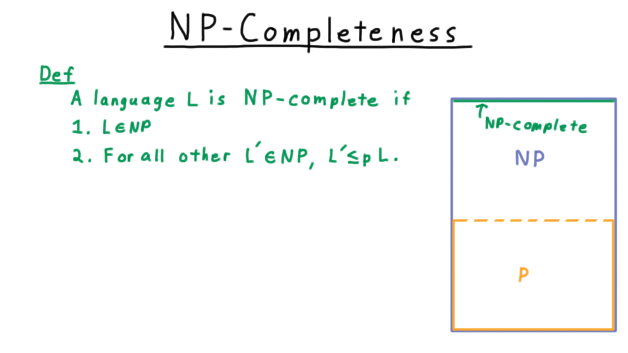
It’s not immediately obvious that an NP-complete problem even exists, but it turns out that there are lots of them and in fact they seem to occur more often in practice than problems than problems in the intermediate zone, which are not NP-complete and so far have not been proved to be in P either.
Historically, the first natural problem to be proved to be NP-Complete is called Boolean formula satisfiability or SAT for short.
SAT is NP-Complete
This was shown to be NP-Complete by Stephen Cook in 1971 and independently by Leonid Levin in the Soviet Union around the same time. The fact that this problem is NP-complete is extremely powerful, because once you have one NP-Complete problem, you just need to reduce it to other problems in NP to show that they too are NP-complete. Thus, much of the theory of complexity can be said to rest on this theorem. This is the high point of our study of complexity.
CNF Satisfiability - (Udacity, Youtube)
For our purposes, we won’t have to work with the most general satisfiability problem. Rather, we can restrict ourselves to a simpler case where the boolean formula has a particular structure called conjunctive normal form, or CNF, like this one here.

First, consider the operators. The \(\vee\) indicates a logical OR, the \(\wedge\) indicates a logical AND, and the bar overtop \(\overline{\cdot}\) indicates logical NOT.
For one of these formulas, we first need a collection of variables, \(x,y,z\) for this example. These variables appear in the formula as literals. A literal can be either a variable or the variable’s negation. For example, the \(x\), or \(\overline{y}\), etc.
At the next higher level, we have clauses, which are disjuctions of literals. You could also say a logical OR of literals. One clause is what lies inside of a parentheses pair.
Finally, we have the formula as a whole, which is a conjunction of clauses. That is to say, all the clauses get ANDed together.
Thus, this whole formula is in conjuctive normal form. In general, there can be more than two clauses that get ANDed together. That covers the terms we’ll use for the structure of a CNF formula.
As for satisfiability itself, we say that
A boolean formula is satisfiable if there is a truth assignment for the formula, a way of assigning the variables true and false such that the formula evaluates to true.
The CNF-satisfiability problem is: given a CNF formula, determine if that formula has a satisfying assignment.
Clearly, this problem is in NP since given a truth assignment, it is takes time polynomial in the number of literals to evaluate the formula. Thus, we have accomplished the first part of showing that satisfiability in NP-complete. The other part, showing that every problem in NP is polynomial-time reducible to it, will be considerably more difficult.
Does it Satisfy - (Udacity)
To check your understanding of boolean expressions, I want you to say whether the given assignment satisfies this formula.
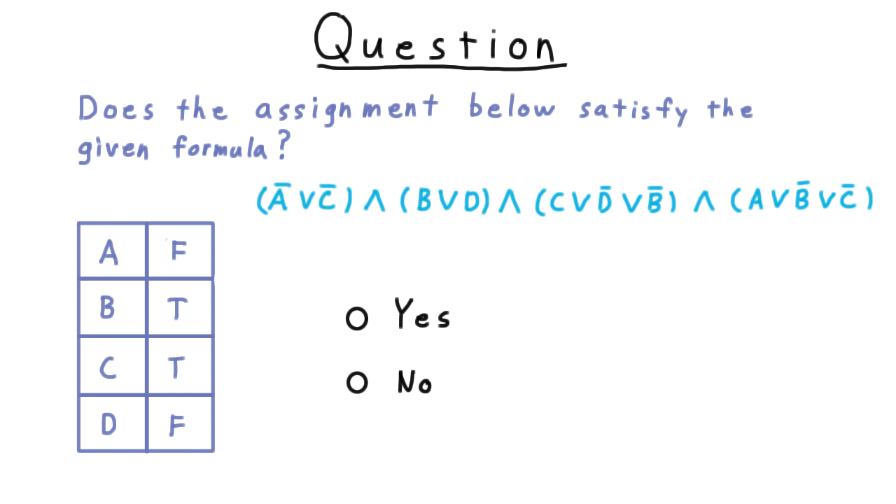
Find a Satisfying Assignment - (Udacity)
Just because one particular true assignment doesn’t satisfy a boolean formula doesn’t mean that there isn’t a satisfying assignment. See if you can find one for this formula. Unless you are a good guesser, this will take longer than just testing whether a given assignment satisfies the formula.
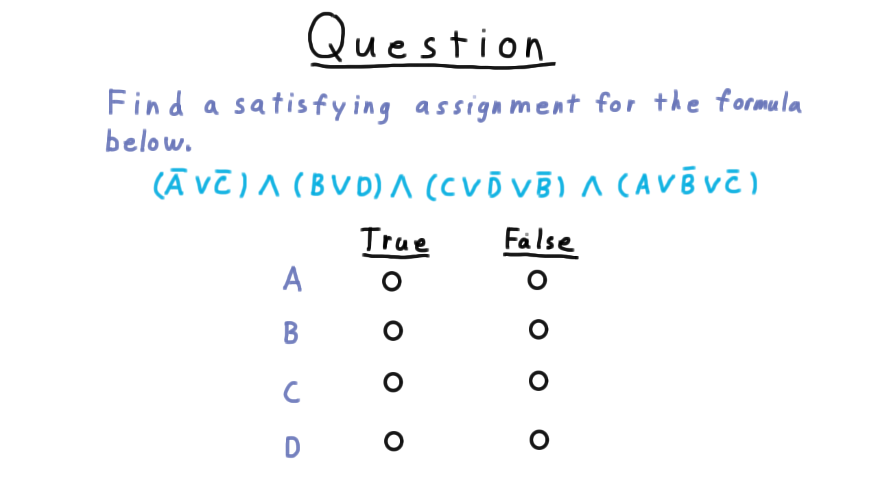
Cook Levin - (Udacity, Youtube)
Now that we’ve understood the satisfiability problem, we are ready to tackle the Cook-Levin theorem. Remember that we have to turn any problem in NP into an instance of SAT, so it’s natural to start with the thing that we know all problems in NP have in common: there is a nondeterministic machine that decides them in polynomial time. That’s the definition after all.
Therefore, let \(L\) be an arbitrary language in NP and let \(M\) be a nondeterministic Turing machine that decides \(L\) in time \(p(n),\) where \(p\) is bounded above by some polynomial.
An accepting computation, or sequence of configurations, for the machine M can be represented in a tableau like this one here.
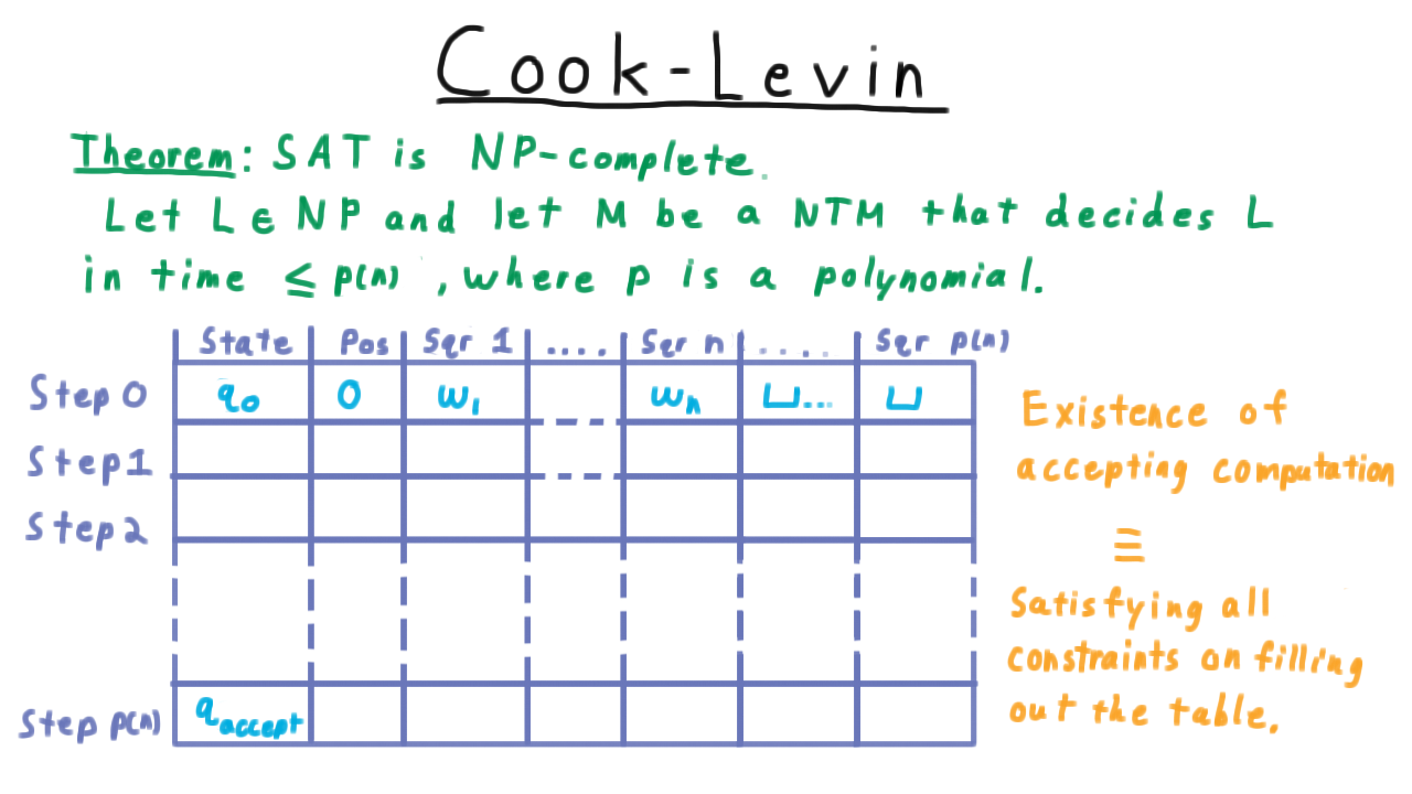
Each configuration in the sequence is represented by a row, where we have one column for the state, one for the head position and then columns for each of the values of the first \(p(n)\) squares of the tape. Note that no other squares can written to because there just isn’t time to move the head that far in only \(p(n)\) steps.
Of course, the first row must represent the initial configuration and the last one must be in an accepting state in order for the overall computation to be accepting.
Note that it’s possible that the machine will enter an accepting state before step \(p(n),\) but we can just stipulate that when this happens all the rest of the rows in the table have the same values. This is like having the accept state always transition to itself. The Cook-Levin theorem them consists of arguing that the existence of an accepting computation is equivalent to being able to satisfy a CNF formula that captures all the rules for filling out this table.
The Variables - (Udacity, Youtube)
Before doing anything else, we first need to capture the values in the tableau with a collection of boolean variables. We’ll start with the state column.

We let \(Q_{ik}\) represent whether after step \(i\), the state is \(q_k.\) Similarly, for the position column, we define \(H_{ij}\) to represent whether the head is over square j after step i. Lastly, for the tape contents, we define \(S_{ijk}\) to represent whether after step \(i,\) the square \(j\) contains the \(k\)th symbol of the tape alphabet.
Note that as we’ve defined these variables, there are many truth assignments that are simply nonsensical. For instance, every one of these \(Q\) variables could be assigned a value of True, but in a given configuration sequence the Turing machine can’t be in all states at all times. Similarly, we can’t assign them to be all False; the machine has to be in some state at each time step. We have the same problems with the head postion variables and the variables for the squares of the tape.
All of this is okay. For now, we just need a way to make sure that any accepting configuration sequence has a corresponding truth assignment, and indeed it must. For any way of filling out the tableau, the corresponding truth assignment is uniquely defined by these meanings. It is the job of the boolean formula to rule out truth assignments that don’t correspond to valid accepting computations.
Configuration Clauses - (Udacity, Youtube)
Having defined the variables, we are now ready to move onto building the boolean formula. We are going to start with the clauses needed so that given a satisfying assignment it’s clear how to fill out the table. Never mind for now about whether the corresponding sequence is has valid transitions. For now, we just want the individual configurations to be well-defined.
First, we have to enforce that at each step the machine is in some state.
Hence for all \(i,\) at least one of the state variables for step \(i\) has to be true.
\[(Q_{i0} \vee Q_{i1} \vee \ldots \vee Q_{ir})\; \forall i\]
Note that \(r\) denotes the number of states here. In this context, it is just a constant. (The input to our reduction is the string that we need to transform into a boolean formula, not the Turing Machine description).
The machine also can’t be in two states at once, so we need to enforce that constraint as well by saying that for every pair of state variable for a give time step, one of the two has to be false.
\[(\overline{Q_{ij}} \vee \overline{Q_{ij'}}) \; \forall i, j\neq j'\]
Together these sets of clauses enforce that the machine corresponding to a satisfying truth assignment is in exactly one state after each step.
For the postion of the head, we have a similar set of clauses. The head has to be over some square on the tape, but it can’t be in two places.
\[(H_{i0} \vee H_{i1} \vee \ldots \vee H_{ip(n)})\; \forall i\]
\[(\overline{H_{ij}} \vee \overline{H_{ij'}}) \; \forall i, j\neq j'\]
Lastly, each square on the tape has to have exactly one symbol. Thus, for all steps \(i\) and square \(j\), there has to be some symbol on the square, but there can’t be two.
\[(\overline{S_{ijk}} \vee \overline{S_{ijk'}}) \; \forall i, k\neq k'\]
So far, we have the clauses
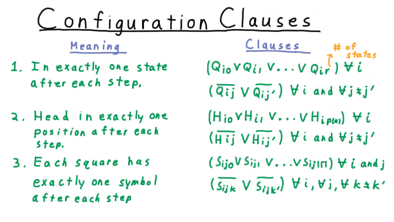
The other clauses related to individual configurations come from the start and end states.
The machine must be in the intial configuration at step 0. This means that the initial state must be \(q_0.\)
The head must also be over the first position on the tape.
The first part of the tape contain the input \(w.\) Letting \(k_1 k_2\ldots k_{|w|}\) be the encoding for the input string, we
The rest of the tape must be blank to start.
These additional clauses are summarized here
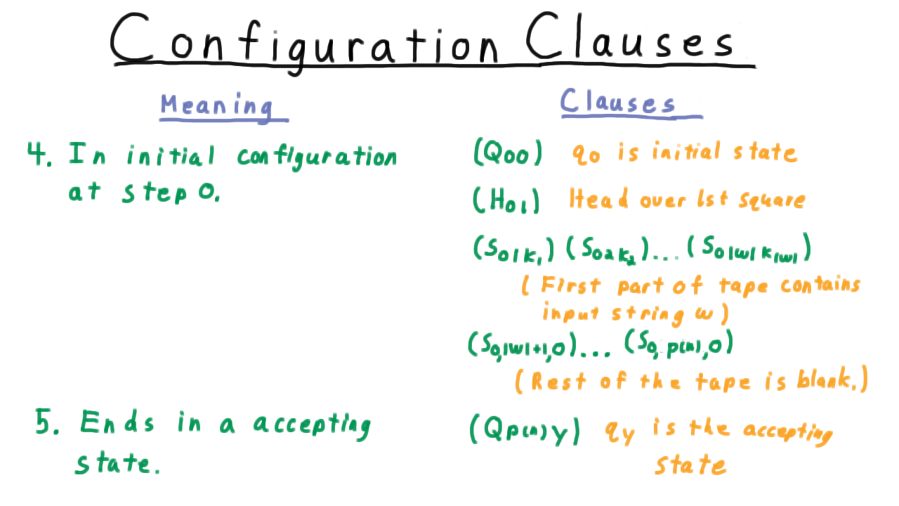
Transition Clauses - (Udacity, Youtube)
Any assignment that truth assignment that satisfies these clauses we have defined so far indicated how the tableau should be filled out. Moreover, the tableua will always start out in the initial configuration and end up in an accepting one. What is not guaranteed yet it that the transitions between the configurations are valid.
To see how we can add constraints that will give us this guarantee, we’ll use this example.
Suppose that the transition functions tells us that if the machine is in state \(q_3\) and it reads a 1. Then it do one of two things:
- it can stay in \(q_0,\) leave the 1 alone, and move the head to the right,
- it can move to state \(q_4,\) write a 0 and move the head to the left.
To translate this rule into clauses for our formula, it’s useful to make a few definitions. First we need to enumerate the tape alphabet so that we can refer to the symbols by number.
Next, we define a tuple \((k,\ell,k',\ell',\delta)\) to be valid if the triple of the state \(q\_\{k'\}\), the symbol \(s\_\{\ell'\}\), and the direction delta is in the set delta of state \(q_k,\)
For example, the tuple \((3,2,0,2,R)\) is valid.
The first two numbers here indicate which transition rule applies (use the enumeration of the alphabet to translate the symbols), and the last three indicate what transition is being made. In this case, it is in the in the set defined by delta, so this is a valid transition.
On the other hand, the transition \((3,0,4,2,R)\) is invalid. The machine can’t switch to state 4, write a 1, and move the head to the right. That’s not one of the valid transitions given that the machine is in state 3 and that it just read a blank.
Now, there are multiple ways to create the clauses needed to ensure that only valid transitions are followed. Many proofs of Cook’s theorem start by writing out boolean expressions that directly express the requirement one of the valid transitions be followed. The difficulty with this approach is that the intuitive expression isn’t in conjunctive normal form and some boolean algebra is need to convert it. That is to say we don’t immediately get an intuive set of short clauses to add to our formula. On the other hand, if we rule out in invalid transitions instead, then we do get a set of short intuitive clauses that we can just add to the formula.
To illustrate, in order to make sure that this invalid transition is never followed, for every step i and position j, we add a clause that starts like this.
\[ (\overline{ H_{ij}} \vee \overline{Q_{i3}} \vee \overline{S_{ij0}} \]
It starts with three literals that ensure the transition rules for being \(q_3\) and reading the blank symbol actually do apply. If the head isn’t in the position we’re talking about, the state isn’t q_3 , or the symbol being read isn’t the blank symbol, then the clause is immediately satisfied. The clause can also be satisfied if the machine behaves in any way that is different from what this particular invalid transition would cause to happen.
\[ \overline{ H_{(i+1)(j+1)}} \vee \overline{ Q_{(i+1)4}} \vee \overline{S_{(i+1)(j+1)2}} ) \]
The head could move differently, the state could change differently, or a different symbol could be written.
Another way to parse this clause is as saying if the \((q_3, \sqcup)\) transition rule applies, then the machine can’t have changed in this particular invalid way. Logically, remember that A implies not B is equivalent to not A or not B. That’s the logic we are using here.
Transition Clauses Cont - (Udacity, Youtube)
Now let’s state the general rule for creating all the transition clauses. Recall that a tuple \((k,\ell,k',\ell',\Delta)\) is valid if switching to state \(q\_\{k'\}\), writing out symbol \(\ell'\) and moving in direction \(\Delta\) is an option given that the machine is currently in state \(q_k\) and reading symbol \(s\_\ell.\)
For every step \(i,\) position \(j,\) and invalid tuple then, we include in the formula this clause. The first part tests to whether the truth assignment is such that the transition rule applies
and the next three ensure that this invalid transition wasn’t followed. This is just the generalization of the example we saw earlier.
Cook Levin Summary - (Udacity, Youtube)
We’re almost done with the proof that satisfiability is NP-complete, but before making the final arguments I want to remind you of what we’re trying to do.
Consider some language in NP, and suppose that someone wants to be able to determine whether strings are in this language. The Cook-Levin theorem argues that because L is in NP, there is a nondeterministic turing machine that decides it, and it uses this fact to create a function computable in polynomial time that takes any input string x and outputs a boolean forumula that is satisfiable if and only if the string x is in L.
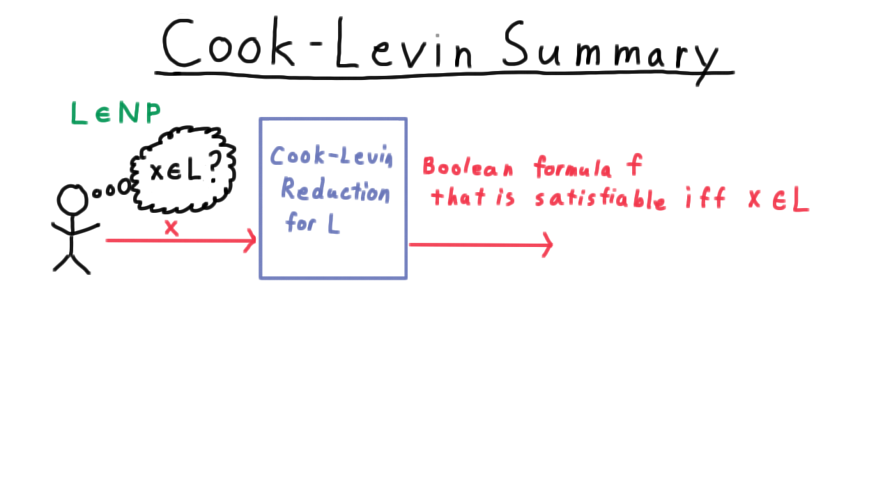
That way, any algorithm for deciding satisfiability in polynomial time would be able to decide every language in NP.
Only two questions remain.
- “Is the reduction correct?”
- “Is it polynomial in the size of the input?”
Let’s consider correctness first. If \(x\) is in the language, then clearly the output formula \(f\) is satisfiable. We can just use the truth assignment that corresponds to an accepting computation of the nondeterministic Turing machine that accepts \(x.\) That will satisfy the formula \(f.\) That much is certainly true.
How about the other direction? Does the formula being satisfiable imply that x is in the language? Take some satisfying assignment for \(f.\) As we’ve argued,
- the corresponding tableau is well-defined. Only one of the state variables can be true at any time step, etc,
- the tableau starts in the initial configuration,
- every transition is valid,
- the configuration sequence ends in an accepting configuration.
That’s all that is needed for a nondeterministic Turing machine to accept, so this direction is true as well.
Now, we have to argue that the reduction is polynomial.
First, I claim that the running time is polynomial in the output formula length. There just isn’t much calculation to be done besides iterating over the combination of steps, head positions, states, and tape symbols and printing out the associated terms of the formula.
Second, I claim that the output formula is polynomial in the input length. Let’s go back and count

These clauses pertaining to the states require order \(p(n) \log n\) string length. The number of states of the machine is a constant in this context. The \(p\) factor comes from the number of steps of the machine. The \(\log n\) factor comes from the fact that we have to distinguish the literals from one another. This requires log n bits. In all these calculations, that’s where the log factor comes from.
For the head position, we have \(O(p(n)3 log n)\) string length one factor of p from the number of time steps and two from all pairs of head positions.
There are \(O(p^2)\) combinations of steps and squares, so this family of clauses requires \(O(p^2 log n)\) length as well.

The other clauses related to individual configurations come from the start and end states. The initial configuration clause is a mere \(O(p(n) \log n)\)
The constraint that the computation be accepting only requires \(O(\log n)\) string length.
The transition clauses might seem like they would require a high order polynomial of symbols, but remember that the size of the nondeterministic Turing machine is a constant in this context. Therefore, the fact that we might have to write out clauses for all pairs of states and tape symbols doesn’t affect the asymptotic analysis. Only the range of the indices i and j depend on the size of the input string, so we end up with \(O(p^2 \log n).\)
Adding all those together still leaves us with a polynomial string length. So, yes, the reduction is polynomial! And Cook’s theorem is proved.
Conclusion - (Udacity, Youtube)
Congratulations!! You have seen that one problem, satisfiability, captures all the complexity of P versus NP problem. An efficient algorithm for Satisfiability would imply P = NP. If P is different than NP then there can’t be any efficient algorithm for satisfiability. Satisfiability has efficient algorithms if and only if P = NP.
Steve Cook, a professor at the University of Toronto, presented his theorem on May 4, 1971 at the Symposium on the Theory of Computing at the then Stouffer’s Inn in Shaker Heights, Ohio. But his paper didn’t have an immediate impact as the Satisfiability problem was mainly of interest to logicians. Luckily a Berkeley professor Richard Karp also took interest and realized he could use Satisfiability as a starting point. If you can reduce Satisfiability to another NP-complete problem than that problem must be NP-complete as well. Karp did exactly that and a year later he published his famous paper on “Reducibility among combinatorial problems” showing that 21 well-known combinatorial search problems that were also NP-complete, including, for example, the clique problem.
Today tens of thousands of problems have been shown to be NP-complete, though ones that come up most often in practice tend to be closely related to one of Karp’s originals.
In the next lesson, we’ll examine some of the reductions that prove these classic problems to be NP-complete, and try to convey a general sense for how to go about finding such reductions. This sort of argument might come in handy if you need to convince someone that a problem isn’t as easy to solve as they might think.
NPC Problems - (Udacity)
Introduction - (Udacity, Youtube)
In the last lecture, we proved the Cook-Levin theorem which shows that CNF Satisfiability is NP-complete. We argued directly that an arbitrary problem in NP can be turned into the satisfiability problem with a polynomial reduction. Of course, it is possible to make such a direct argument for every NP-complete problem, but usually this isn’t necessary. Once we have one NP-complete problem, we can simply reduce it to other problems to show that they too are NP-complete.
In this lesson, we’ll use this strategy to prove that a few more problems are NP-complete. The goal is to give you a sense of the breadth of the class of NP-complete problems and to introduce you to some of the types are arguments used in these reductions.
Basic Problems - (Udacity, Youtube)
Here is the state of our knowledge about NP-complete problems given just what we proved in the last lesson.

We’ve shown that we can take an arbitrary problem in NP and reduce it to CNF satisfiability–that is what the Cook-Levin theorem showed.
We also did another polynomial reduction, one of the Independent Set/Clique problem to the Vertex Cover problem. Again, I’m treating Independent Set and Clique here as one, because the problems are so similar. Much of this lesson will be concerned with connecting up these two links into a chain.
First we are going to reduce general CNF-SAT to 3-SAT where each clause has exactly three literals. This is a critical reduction because 3-SAT is much easier to reduce to other problems than general CNF. Then we are going to reduce 3-CNF to Independent Set, and by transitivity this will show that vertex cover is NP-complete. Note that this is very convenient because it would have been pmessy to try to reduce every problem in NP to these problems directly. Finally, we will reduce 3-CNF to the Subset Sum problem, to give you a fuller sense of the types of arguments that go into reductions.
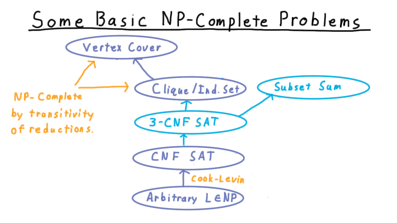
CNF 3CNF - (Udacity)
First we are going to reduce general CNF-SAT to 3-CNF-SAT. Before we begin however, I want you to help me articulate what we are trying to do. Here is a question. Choose from the options at the bottom and enter the corresponding letter in here so that this description matches the reduction we are trying to achieve.
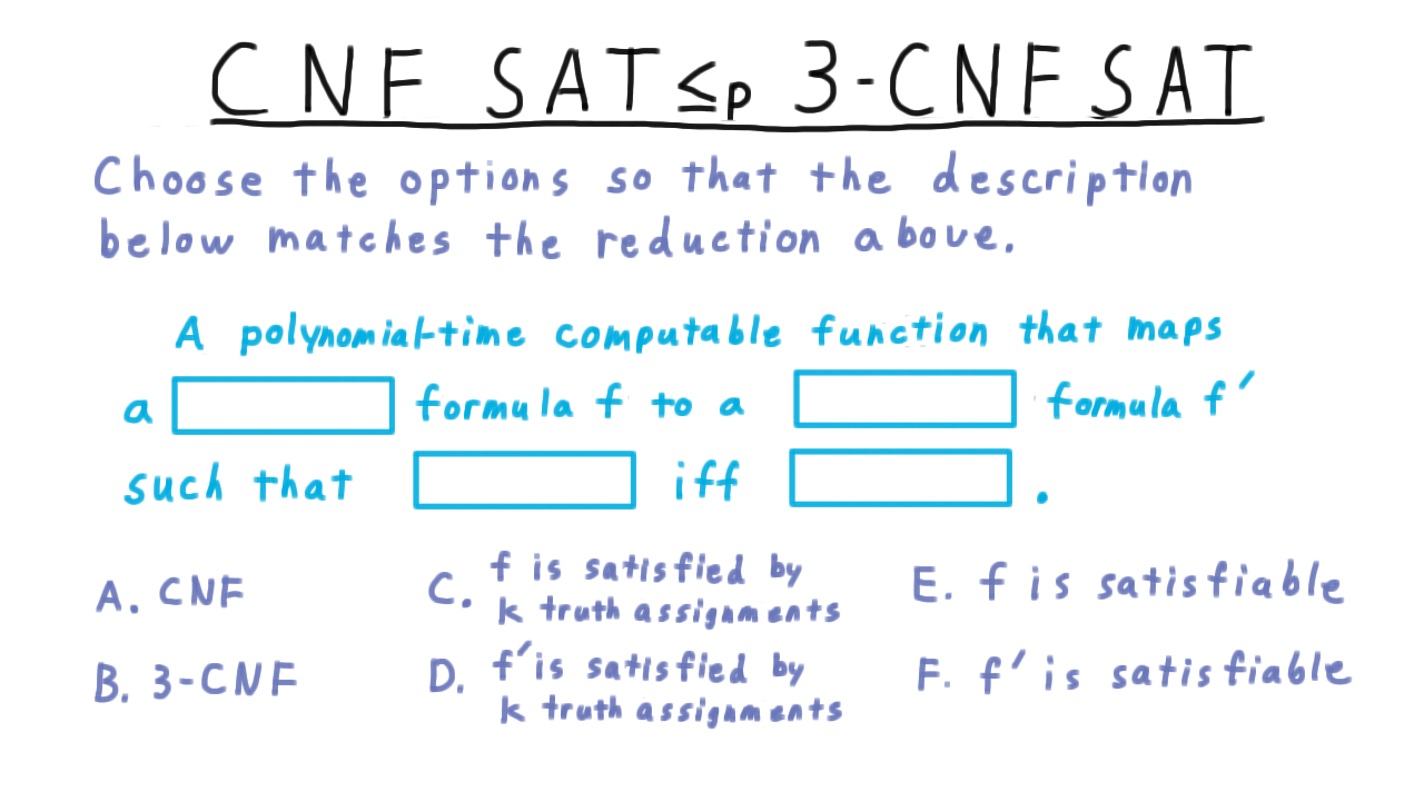
Strategy and Warm up - (Udacity, Youtube)
Here is our overall strategy. We’re going to take a CNF formula \(f\) and turn it into a 3CNF formula \(f',\) which will includes some additional variables, which we’ll label \(Y.\) This formula \(f'\) will have the property that for any truth assignment \(t\) for the original formula \(f,\) \(t\) will satisfy \(f\) if and only if there is a way \(t_Y\) of assigning values to \(Y\) so that \(t\) extended by \(t_Y\) satisies \(f'.\)
Let’s illustrate such a mapping for a simple example. Take this disjunction of 4 literals.
\[(z_1 \vee z_2 \vee z_3 \vee z_4) \]
Note that the \(z_i\) are literals here, so they could be \(x_1\) or \(\overline{x_1}\), etc. Remember too that disjunction means logical OR; the whole clause is true if any one of the literals is.
We will map this clause of 4 into two clauses of 3 by introducing a new variable \(y\) and forming the two clauses
\[(z_1 \vee z_2 \vee \overline{y}) \wedge (y \vee z_3 \vee z_4).\]
Let’s confirm that the desired property holds. If the original clause is true, then we can set \(y\) to be \(z_1 \vee z_2\). If \(z_1 \vee z_2\) is true, then this first clause will be true by itself, and \(y\) can satisfy the other clause. Going the other direction, suppose that we have a truth assignment that satisfies both of these clauses. Suppose first that \(y\) is true. That implies that \(z_1 \vee z_2\) is true and therefore, the clause of four literals is. Next, suppose that \(y\) is false. Then \(z_3\) or \(z_4\) must true, and again so must the clause of four. If you have understood this, then you have understood the crux of why this reduction works. More details to come.
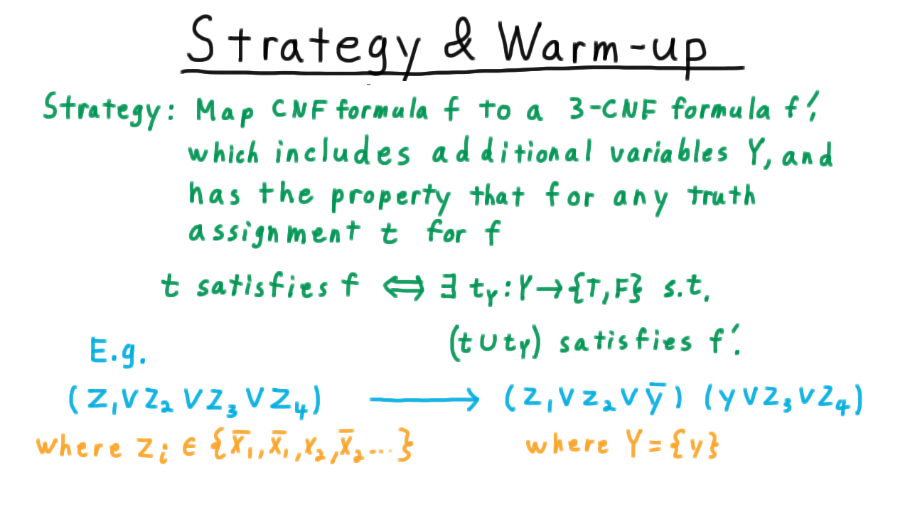
Transforming One Clause - (Udacity, Youtube)
We are going to start by looking at how to convert just one clause from CNF to 3-CNF. This is going to be the heart of the argument, because we will be able to apply this procedure to each clause of the formula independently. Therefore, consider one clause consisting of literals \(z_1\) through \(z_k.\) We are going to have four cases depending on the number of literals in the clause.
The case where \(k=3\) is trivial since nothing needs to be done.
When there are two literals in a clause, the situation is as simple trick suffices. We just need to boost up the number of literals to three. To do this, we include a single extra variable and trade in the clause
\[ (z_1 \vee z_2)\]
for these two clauses,
\[ (z_1 \vee z_2 \vee y_1) \wedge (z_1 \vee z_2 \vee \overline{y_1})\]
one with the literal \(y_1\) and one with the literal \(\overline{y_1}.\) If in a truth assignment \(z_1 \vee z_2\) is satisfied, then clearly both of these clauses have to be true. On the other hand, taking a satisfying assignment for the pair of clauses, the y-literal has to be false in one of them, so \(z_1 \vee z_2\) must be true.
We can play the same trick when there is just one literal \(z_1\) in the original clause. This time we need to introduce two new variables, which we’ll call \(y_1\) and \(y_2.\) Then we replace the original clause with four. See the chart below.
Note that if \(z_1\) is true, then all of collection of four clauses are true too. On the other hand, for any given truth assignment for \(z_1, y_1,\) and \(y_2\) that satisfies these clauses, the y-literals will have both be false in one of the four clauses. Therefore, \(z_1\) must be true.
Lastly, we have the case where \(k > 3\). Here we introduce \(k-3\) variables and use them to break up the clauses according to the pattern shown above.
Let’s illustrate the idea with this example
\[(z_1 \vee z_2 \vee z_3 \vee z_4 \vee z_5 \vee z_6).\]
Looking at this we might wish that we could have a single variable that captured whether any one of these first 4 variables were true. Let’s call this variable \(y_3.\) Then we could express this clause in as the 3 literal clause
\[(y \vee z_5 \vee z_6).\]
At first, I said we wanted \(y_3\) would to be equal to \(z_1 \vee z_2 \vee z_3 \vee z_4,\) but it’s actually sufficient, and considerably less trouble, for \(y_3\) to just imply it. This idea is easy to express as a clause.
\[(z_1 \vee z_2 \vee z_3 \vee z_4 \vee \overline{y})\]
Either y is false, in which case this implication doesn’t apply, or one of \(z_1\) through \(z_4\) better be true. Together, these two clauses imply the first one. If \(y\) is true, then one of \(z_1\) through \(z_4\) is, and so is the original. And if \(y\) is false, then \(z_4\) or \(z_5\) is true and so is the original.
Also, if there original is satisfied, then we can just set \(y_3\) equal to the disjuction of \(z_1\) through \(z_4\) and these two clauses will be satisfied as well.
Note that we went from having a longest clause of length 6 to having one of length 5 and another of length 3. We can apply this strategy again to the clause that is still too long. We introduce another variable \(y_2\) and trade this long clause in for a shorter clause and another one with three literals. Of course, we can then play this trick again, and eventually, we’ll have just 3-literal clauses.
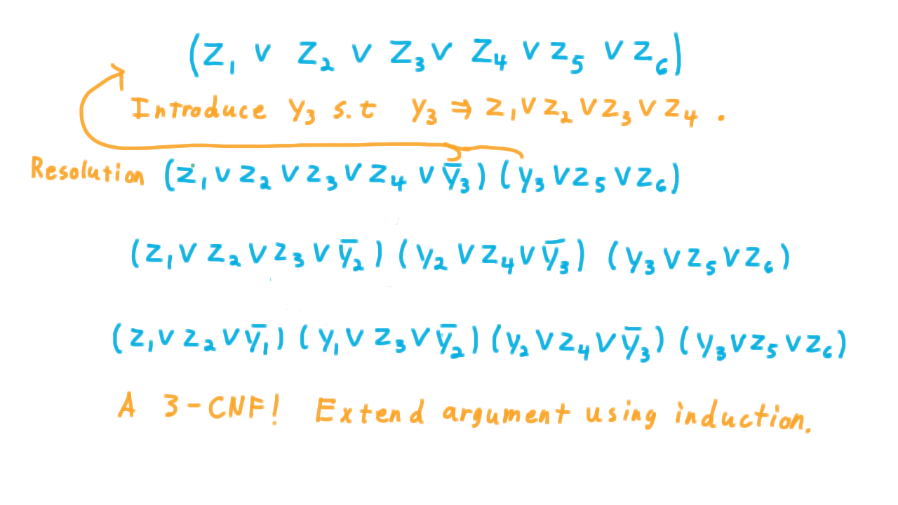
The example is for k=6, but an inductive argument will show that the argument works for any k greater than 3.
Extending A Truth Assignment - (Udacity)
Here is an exercise intended to help you solidify your understanding of the relationship between the original clause and the set of 3 clauses that the transformation produces. I want you to extend the truth assignment below so that it satisfies the given 3CNF formula. This one is the image of this clause here under the transformation that we’ve discussed.
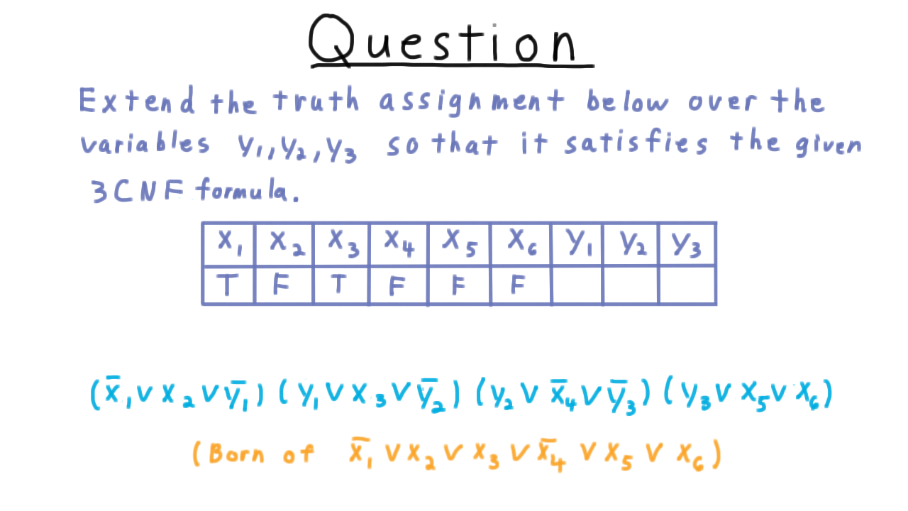
CNF SAT - (Udacity, Youtube)
Recall that our original purpose was to find a transformation of the formula such that an truth assignment satisfied the original if and only if it could be extended to the transformed formula.

We’ve seen how to do this transformation for a single clause, and actually this is enough. We can just transform each clause individually introducing a new set of variables for each; all of the same argument about extending or restricting the truth assigment will hold.
Let’s illustrate what a transformation of multi-clause formula looks like with an example. Consider this formula here,
\[(z_{11} \vee z_{12}) \wedge (z_{21} \vee z_{22} \vee z_{23} \vee z_{24} \vee z_{25}) \]
where I’ve indexed the literals \(z\) with two indices now, the first refering to the clause it’s in and the second being its enumeration within the clause.
The first clause only has two literals, so we transform it into these two clauses with 3 literals by introducing a new variable \(y_{11}.\) It gets the first 1 because it was generated by the first clause.
We transform this second clause with 5 literals into these three clauses introducing the two new variables \(y_{21}\) and \(y_{22}\). Note that these are different from the variables used in the clauses generated by the the first original clause. Since all of these sets of variables are disjoint, we can assign them independently of each other and apply all the same arguments as we did to individual clauses. The results are shown below.
That’s how CNF can be reduced to 3CNF. This transformation runs in polynomial time, making the reduction polynomial.
We just reduced the problem of finding a satisfying to a CNF formula to the problem of finding a satisfying assignment to a 3CNF formula. At this point, it’s natural to ask, “can we go any further? Can we reduce this problem to a 2CNF?” Well no, not unless P=NP. There is a polynomial time algorithm for finding a satisfying a 2-CNF formula based on finding strongly connected components. Therefore, If we could reduce 3-CNF to 2CNF, then P=NP.
So 3CNF is as simple as the satisfiability question gets, and it admits some very clean and easy-to-visualize reductions that allow us to show that other problems are in NP. We’ll go over two of these: first, the reduction to independent set (or clique) and then to Subset Sum.
3CNF INDSET - (Udacity, Youtube)
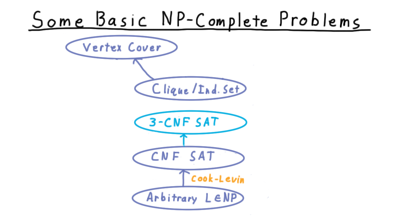
A the beginning of the lesson, we promised that we could link up these two chains and use the transitivity of reductions to show that Vertex Cover and Independent Set were NP-complete. We now turn to the last link in this chain and will reduce 3CNF-SAT to Independent Set. As we’ve already argued these problems are in NP, so that will complete the proofs.
Here then is the transformation, or reduction, we need to accomplish. The input is a 3CNF formula with m clauses, and we need to output a graph that has an independent set of size m if and only if the input is satisfiable.
We’ll illustrate on this example.
\[(a \vee b \vee c) \wedge (\overline{b} \vee c \vee d) \wedge (a \vee \overline{b} \vee \overline{c})
For each literal in the formula, we create a vertex in a graph. Then we add edges between all vertices that came from the same clause. We'll refer to these as the within-clause edges or simply the clause edges. Then we add edges between all literals that are contradictory. We'll refer to these as the between-clause edges or the contradiction edges.
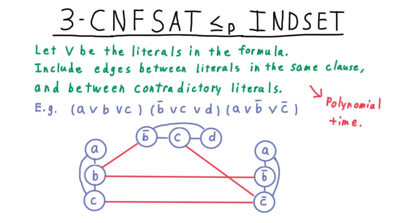
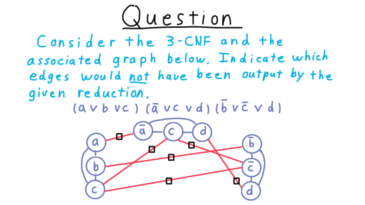
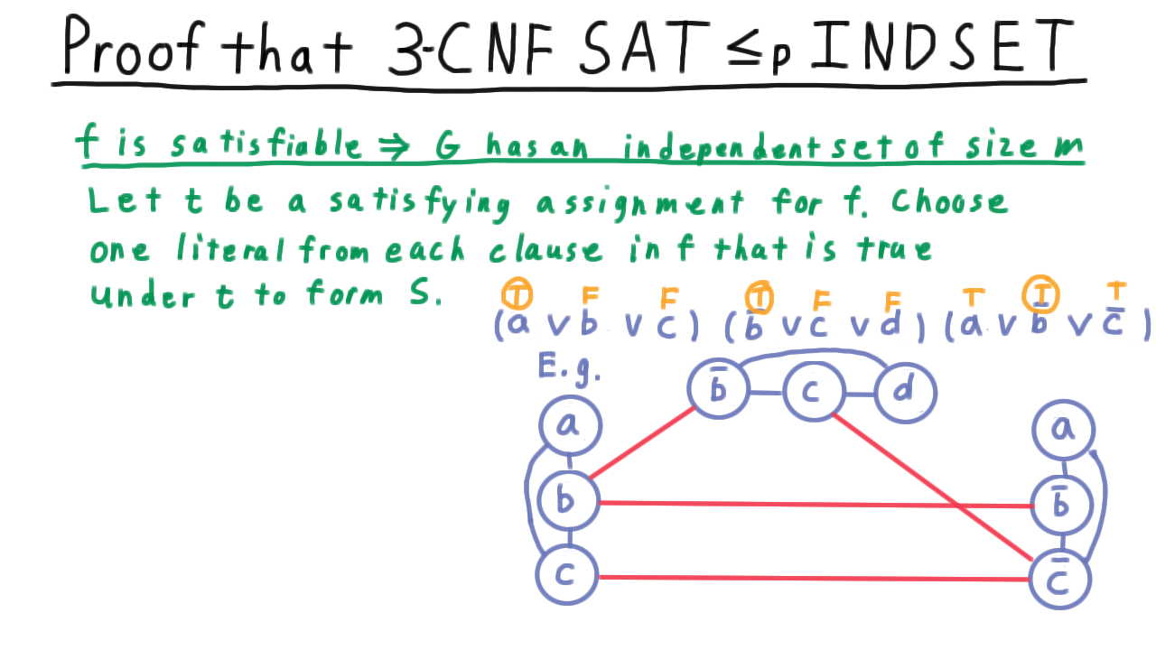
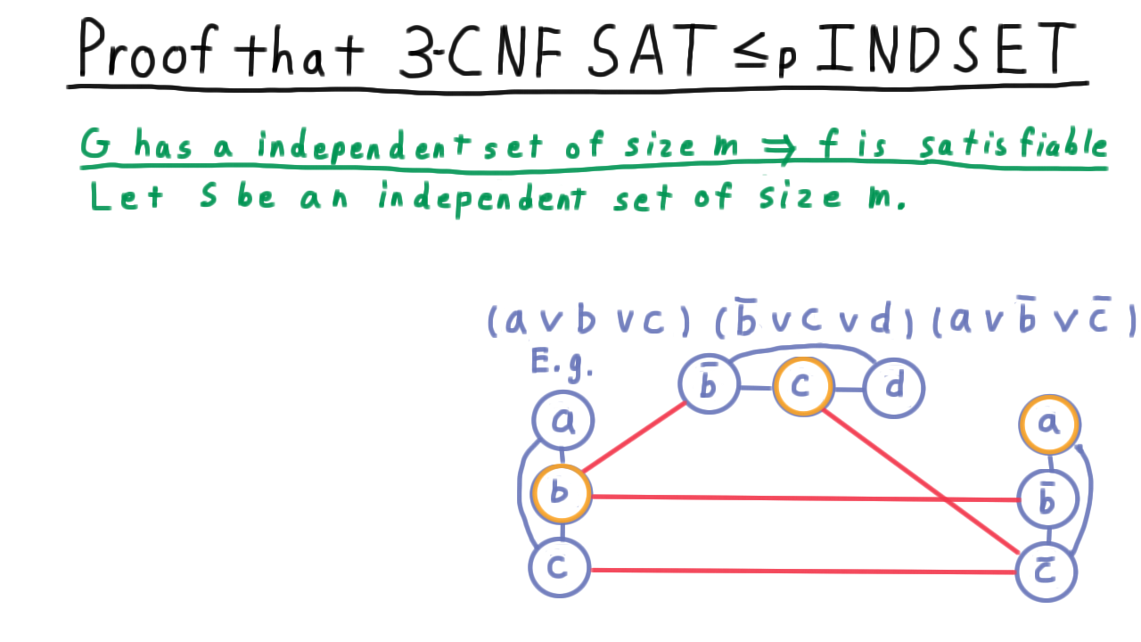
showing that both Independent Set and Vertex Cover are NP-complete.
Next, we are going to branch out both in the tree here and in the types of arguments we’ll make by considering the subset sum problem.
Subset Sum - (Udacity, Youtube)
Before reducing 3CNF to Subset Sum, we have to define the Subset Sum problem first. We are given a multiset of \(\\{a_1, \ldots, a_m\\}\), where each element is a positive integer. A multiset, by the way, is just a set that that allows the same element to be included more than once. Thus, a set might contain three 5s, two 20s and just one 31, for example. We are also given a number \(k.\) The problem is to decide whether there is a subset of this multiset whose members add up to \(k.\)
One instance of this problem is partitioning, and I’ll use this particular example to illustrate.
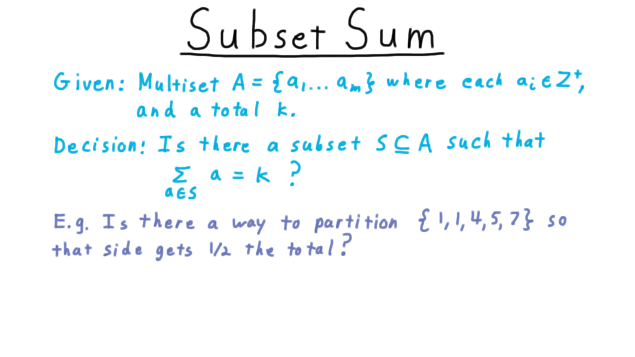
Imagine that you wanted to divide assets evenly between two parties–maybe we’re picking teams on the playground, trying to reach a divorce settlement, dividing spoils among the victors of war, or something of that nature. Then the question becomes, “Is there a way to partition a set so that things come out even, each side getting exactly 1/2?”
In this case, the total is 18, so we could choose \(k\) to be equal to 9 and then ask if there is a way to get a subset to sum to 9.
Indeed, there is. We can choose the two 1’s and the 7, and that will give us 9. Choosing 4 and 5 would work too, of course.
That’s the subset sum problem then. Note that the problem is in NP because given a subset, it takes polynomial time to add up the elements and see if the sum equals k. Finding the right subset, however, seems much harder. We don’t know of a way to do it that is necessarily faster than just trying all 2m subsets.
A Subset Sum Algorithm - (Udacity)
We are going to show that Subset Sum is NP-complete, but here is a simple algorithm that solves it. \(W\) is a two-dimensional array of booleans
and \(W[i][j]\) indicates whether there is a subset of the first \(i\) elements that sums to \(j.\) There are only two ways that this can be true:
- either there is a way to get \(j\) using only elements \(1\) through \(i-1,\)
- or there is a way to get \(j-a_i\) using the first \(i-1,\) and then we include \(a_i\) to get \(j.\)
For now, I just want you to give the the tightest valid bound on the running time for a Random Access Machine.
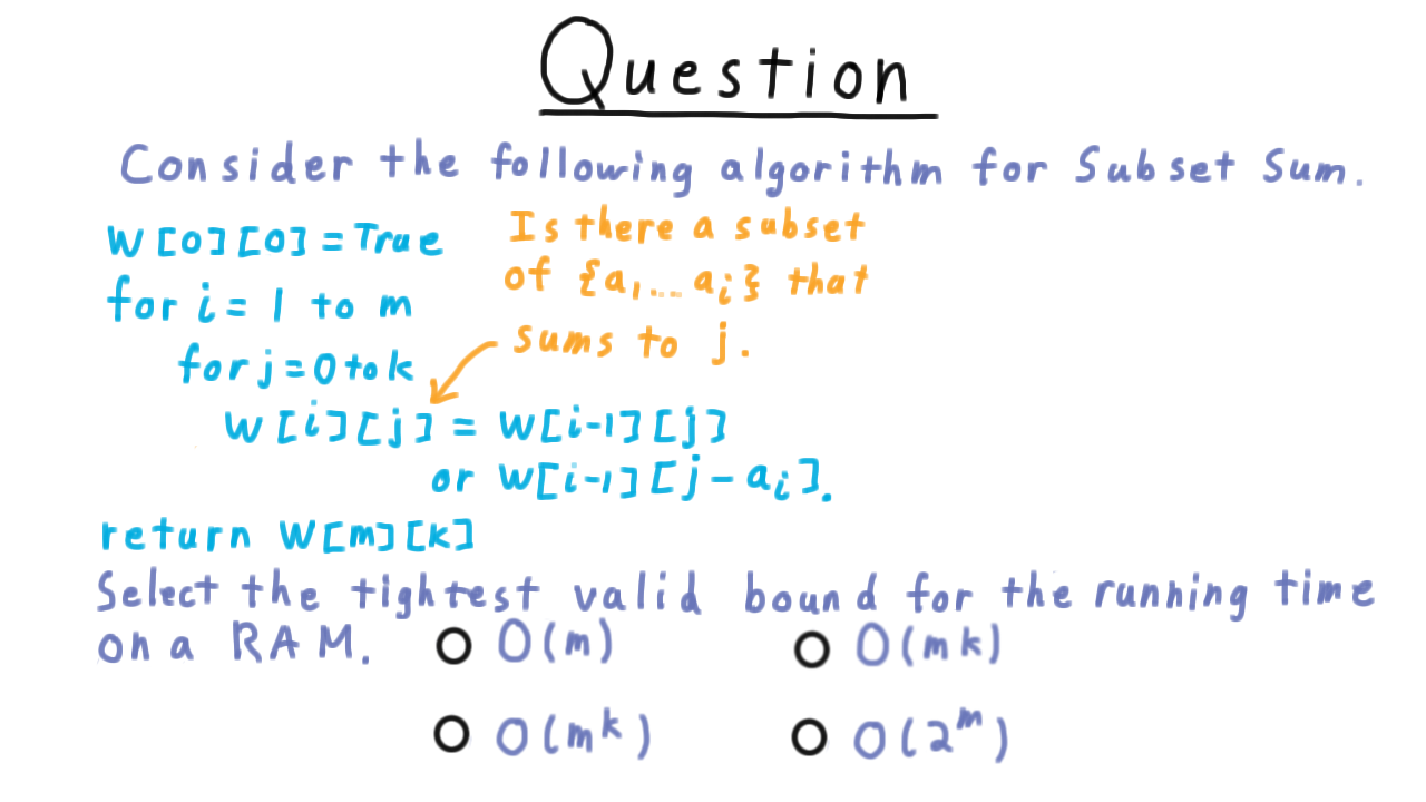
3 CNF Subset Sum - (Udacity, Youtube)
Here is the reduction of 3-CNF SAT to Subset Sum. We’ll illustrate the reduction with an example, because writing out the transformation in its full generality can get a little messy. Even with just an example, the motivation for the intermediate steps might not be clear at the time. It should all become clear at the end, however.
We’re going to create a table with columns for the variables and columns for the clauses. The rows of the table are going to be numbers in our subset, and we’ll have this column represent the ones place, this one the tens place, and so forth.
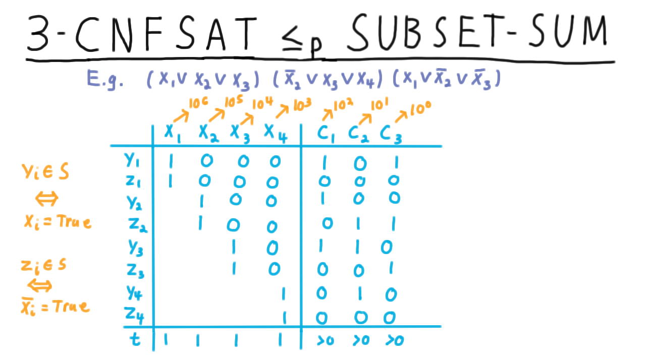
The collection of numbers will consist of two numbers for every variable in the formula: one that we include when t(x_i) is true–we’ll notate those with y– and another that we include when it is false–we’ll notate those with z.
In the end, we want to include either \(y_i\) or \(z_i\) for every \(i,\) since we have to assign the variable \(x_i\) one way or the other. To get a satisfying assignment, we also have to satisfy each clause, so we’ll want the numbers \(y_i\) and \(z_i\) to reflect which clauses are satisfied as well. The number \(y_1\) sets \(x_1\) to true, so we put a 1 in that column to indicate that choosing \(y_1\) means assigning \(x_1\). Since this assigns \(x_1\) to be true, it also means satisfying clauses 1 and 3 in our example.
Choosing \(z_1\) also would assign the variable \(x_1\) a value, but it wouldn’t satisfy any clauses. Therefore, that row is the same as for \(y_1\) except in the clause columns where are all set to zero.
We do the analogous procedure for \(y_2\) and \(z_2\): the literal \(x_2\) appears in clause 1, and the literal \(\overline{x_2}\) appears in clauses 2 and 3. We can do the same for variables \(x_3\) and \(x_4.\) These then are the numbers that we want to include in our set A.
It remains to choose our desired total \(k.\) For each of these variable columns the desired total is exactly 1. We assign each variable one way or the other. For these clause columns, however, the total just has to be greater than 0. We just need one literal in the clause to be true in order for the clause to be satisfied. Unfortunately, that doesn’t yield a specific \(k\) that we need to sum to.
The trick is to add more numbers to the table.
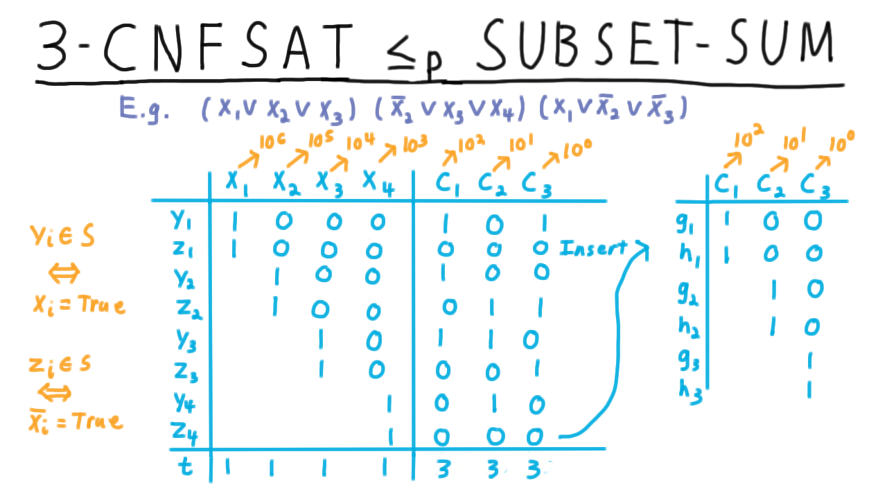
These all have zeros in the places corresponding to the variables, and exactly one 1 in a column for a clause. Each clause \(j\) gets two numbers that have a 1 in the \(j\)th column. We’ll call them \(g_j\) and \(h_j.\)
This allows us to sse the desired number to be 3 in the clause columns. Given a satisfying assignment, the corresponding choice of \(y\) and \(z\) numbers will have at least a 1 in all the clause columns but no more than 3. All the 1’s and 2’s can be boosted up by including the \(g\) and \(h\) numbers. Note that if some clause is unsatisfied, then include the \(g\) and \(h\) numbers isn’t enough to bring the total to 3 because there are only two of them.
That’s the construction. For each variable the set of number to choose from includes two numbers \(y\) and \(z\) which will correspond to the truth setting, and for each clause it includes \(g\) and \(h\) so that we can boost up the total in the clause column to three where needed.
This construction just involves a few for-loops, so it’s easy to see that the construction of the set of numbers is polynomial time.
Proof that 3CNF SUBSET SUM - (Udacity, Youtube)
Next, we prove that this reduction works. Let \(f\) be a 3CNF formula with \(n\) variables and \(m\) clauses. Let \(A\) be the multiset over the positive integers and \(k\) be the total number output by the transformation.
First, we show that if \(f\) is satisfiable then there is a subset of \(A\) summing to \(k.\) Let \(t\) be the satisfying assignment. Then we include \(y_i\) in \(S\) if \(x_i\) is true under t, and we’ll include \(z_i\) otherwise. As for the \(g\) and \(h\) families of numbers, if there are fewer than three literals of clause j satisfied under \(t,\) then include \(g_j.\) If there are a fewer than 2, then include \(h_j\) as well. In total, the sum of these numbers must be equal to \(k.\)
In the other direction, we argue that if there is a subset of \(A\) summing to \(k,\) then there is a satisfying assignment. Suppose that \(S\) is a subset of \(A\) summing to \(k.\) Then the impossibility of any “carrying” of the digits in any sum implies that exactly 1 of \(y_i\) or \(z_i\) must have been set to true. Therefore, we can define a truth assignment \(t\) where \(t(x_i)\) is true if \(y_i\) is included in \(S\) and false otherwise. This must satisfy every clause; otherwise, there would be no way that the total in the clause places would be 3.
Altogether, we’ve seen that Subset Sum in NP and we can reduce 3-CNF SAT an NP-complete problem to it, so Subset Sum must be NP-complete.
Other Bases - (Udacity)
Here is an exercise to encourage you to consider carefully the reduction just given. We interpreted the rows of the table we constructed as the base 10 representation of the collection of numbers that the reduction output. What other bases would have worked as well? Check all that apply.
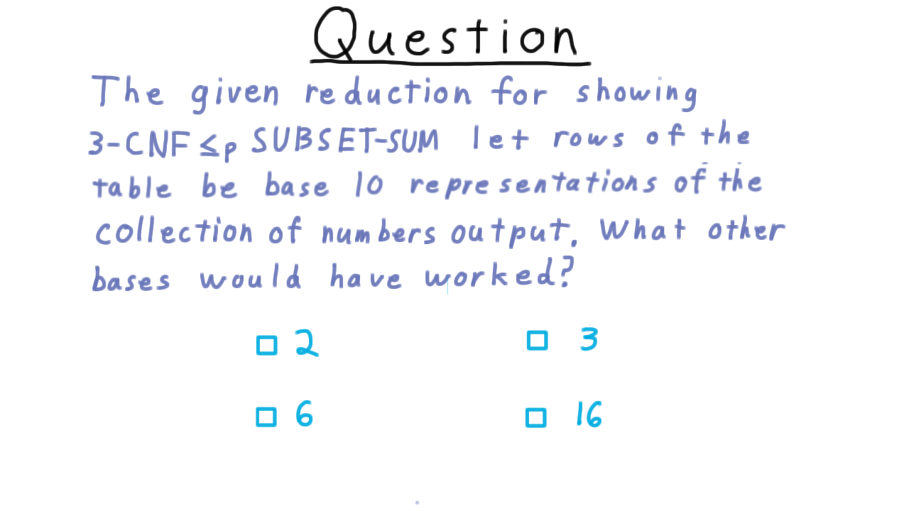
Conclusion - (Udacity, Youtube)
So far, we’ve built up a healthy collection of NP-complete complete problems, but given that there are thousands of problems know to be NP-complete, we’ve only scratched the surface of what is known. In fact, we haven’t even come close to Karp’s mark of 21 problems from his 1972 paper.
If you want to go on and extend the set of problems that you can prove to be NP-complete, you might consider reducing subset sum to the Knapsack problem, where one has a fixed capacity for carrying stuff and want to pack the largest subset of items that will fit.
Another classic problem is that of the Traveling Salesman. He has a list of cities that he wants to visit and, he wants to know the order that will minimize the distance that he has to travel. One can prove that this problem is NP-complete by first reducing Vertex Cover to the Hamiltonian Cycle problem—which asks if there is a cycle in a graph that visits each vertex exactly once—and then Hamiltonian Cycle to Traveling Salesman.
Another classic problem that is used to prove other problems are NP-complete is 3D-matching. 2D matching can be thought of as the problem making as many compatible couples as possible from a set of people. 3D matching extends this problem by further matching them with a home that they would enjoy living in together.
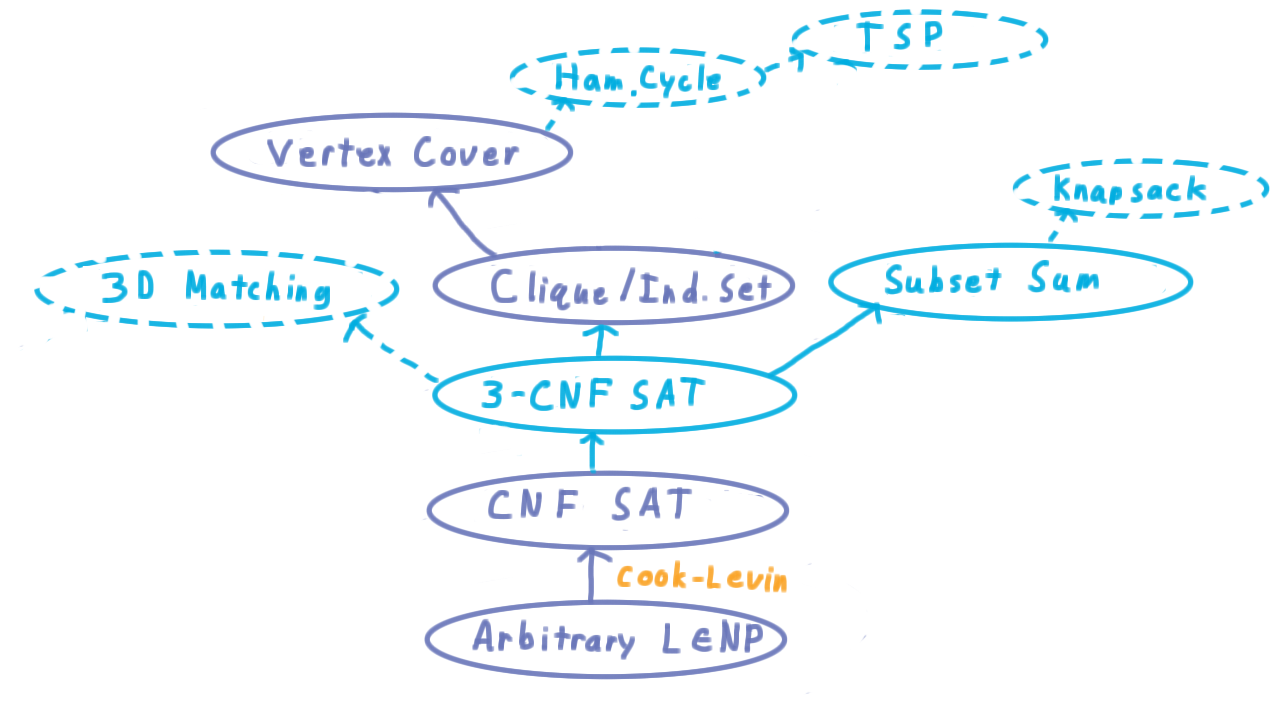
Of course, there are many others. The point of this lesson, however, is not so that you can produce the needed chain of reductions for every problem known to be NP-complete. Rather, it is to give you a sense for what these arguments look like and how you might go about making such an argument for a problem that is of particular interest to you.
The reductions we’ve given as examples are a fine start, but if you want to go further in understanding how to use complexity to understand real-world problems, take a look at the classic text by Garey and Johnson on Computers and Intractability. Even though it is from the same decade as the original Cook-Levin result and Karp’s list of 21 NP-complete problems, it is still one of the best. As Lance, says “a good computer scientist shouldn’t leave home without it.”