Introduction
SPlin was a VolgaCTF 2023 Quals task, category crypto. Unfortunately, the task remained unsolved.
In chapters 1-7 we’ll discuss in detail all the step of the implied solution. To skip it and get straight to the summary of the solution go to TL;DR chapter.
Accompanying this writeup is the solution script solution.py, which contains the working (and tested 😊) implementation of the attack. Some parts are missing and marked === YOUR CODE HERE === for the reader to fill in the blanks and decrypt the flag.
Throughout the writeup we somewhat misleadingly use:
-
"subkey" for "part of a round key",
-
\(0\)-based indexing to count round numbers while still calling round \(0\) "the first round",
-
"chained linear approximation" instead of subjectively more usual "aggregated linear approximation".
1. Info gathering
Inspecting the given files
We start by inspecting the given files:
-
flag.txt.enc -
test.bin.enc -
splin.py
The first two binary files are, judging by their names, encrypted versions of some files named flag.txt and test.bin, respectively. The third file is the cipher script.
Since two ciphertext files are given we may assume the given cipher is not susceptible to COA (ciphertext only attack), although this might not be the case. Also, the ciphertext files differ in size: \(48\) bytes vs. \(275\) kB.
Examining splin.py
Let’s examine the cipher script.
In this Python script we see two large code regions, Cipher implementation and Tests, and __main__ pseudo function.
Cipher implementation region
First we see eight S-boxes SBOX*, which we denote as \(S_0\) though \(S_7\), defined as a list of \(256\) different values ranging from \(0\) to \(255\), that is, a permutation. Therefore, each defines an invertible mapping of an \(8\)-bit input into an \(8\)-bit output.
Below there are two P-boxes PBOX and PBOX2, hereafter \(P\) and \(P_2\), both defined as permutations of length \(64\).
Then there is a code snippet that builds inverted S-boxes SBOX*_inv (denoted as \(S_0^{-1}\) through \(S_7^{-1}\)), and inverted P-box PBOX_inv (\(P^{-1}\)).
These definitions are followed by two functions, sboxes and sboxes_inv, that split an input \(64\)-bit integer \(x\) into eight \(8\)-bit parts \(x_i\), pass these parts through \(S_i\) or \(S_i^{-1}\), respectively, and combine the images \(S_i\mathopen{}\left(x_i\right)\mathclose{}\) or \(S_i^{-1}\mathopen{}\left(x_i\right)\mathclose{}\) into a single output \(64\)-bit integer. Let’s denote these operations as \(S\mathopen{}\left(x\right)\mathclose{}\) and \(S^{-1}\mathopen{}\left(x\right)\mathclose{}\).
The following three functions, pbox, pbox2, and pbox_inv, apply the permutations \(P\), \(P_2\), and \(P^{-1}\), respectively, to the bits of an input \(64\)-bit integer.
Skipping make_keys for now we see functions encrypt_block and decrypt_block. These are the core encryption and decryption functions. encrypt_block takes a \(64\)-bit integer and a set of round keys and sequentially apply the S-boxes, the P-box, and xor with a round key. decrypt_block reverses the process.
Obviously, this cipher is just a regular SP-net [1] (barring some minor differences), which is also hinted at by SP in the cipher’s name SPlin. Its sketch is shown in Figure 1.
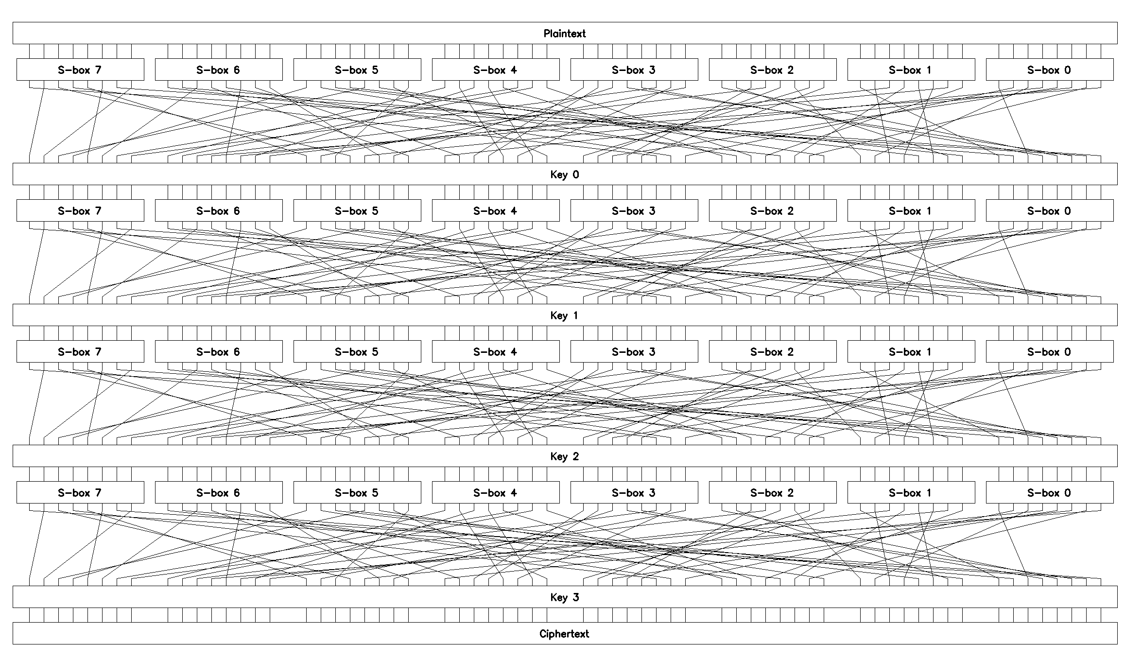
SPlinThe remaining functions encrypt and decrypt define encryption/decryption of input bytes in CBC-mode [2], encrypt_file and decrypt_file wrap these two and handle reading and writing data from and to files.
Tests region
Most of the test functions check if everything works correctly, e.g. if the S-boxes are actually invertible or whether encrypted data can be decrypted.
Only two functions draw attention: check_key_schedule and check_encryption_file. We describe them in the following sections.
The key schedule
Examining function make_keys we see that the cipher expects a \(256\)-bit input key as a hex string.
Having unhexlified the input key make_keys splits it into four \(64\)-bit parts and applies the second permutation \(P_2\) to each of these parts, combine then into byte array of length \(32\), makes a circular shift by \(4\) bytes, and, finally, splits the array into four \(64\)-bit integers to give the round keys.
As can be easily verified this is just a \(256\)-bit permutation. The test function check_key_schedule defines an inversion function and applies excessive checks.
Effectively, a \(256\)-bit key is used to produce four \(64\)-bit round keys, meaning the key schedule in a trivial one, and we can’t expect any weak keys resulting from it.
Therefore, to break SPlin we need to retrieve all the \(256\) bits of the key, thus brute-forcing seems impractical.
check_encryption_file
Perhaps, the most valuable information we get examining the test function check_encryption_file.
First of all, we see this function generates some random bytes, encrypts them and saves the ciphertext as file test.bin.enc. It then checks that this ciphertext can be correctly decrypted.
As we are given file named test.bin.enc we can safely assume this function was used to generate it (examining __main__ also shows that it can be spawned by running the cipher script with python3 splin.py test).
As for the missing plaintext file test.bin, it’s generated by python’s random.randbytes function after having seeded the PRNG with value \(42\):
542
543
544
545
    random.seed(42)
    plaintext = random.randbytes(n_known_pairs * BS)
    with open('test.bin', 'wb+') as f:
        f.write(plaintext)
Hence, we can execute this code snippet to get the missing plaintext.
The length of the plaintext is not random, but given by a curiously-looking expression:
539
540
    e = (1 << 2) * (0.477 * 0.438 * 0.117)
    n_known_pairs = int(8 * (1 / e) ** 2 * 42 + 0.5)
The first expression looks pretty much like a bias of an aggregated (chained) linear approximation given by the so-called Piling-up Lemma [3]:
where \(n\) is the number of linear approximations being aggregated.
The theory also gives an estimate of the expected number of known plaintext-ciphertext pairs required for the approximation to hold [3]:
Thus, n_known_pairs equals \(42\) times the expected number of known plaintext-ciphertext pairs:
Along with the ability to regenerate the plaintext, which gives a lot of known plaintext-ciphertext pairs, and yet another hint in the task’s name SPlin, these formulas lead us to conclusion that the cipher is susceptible to linear cryptanalysis.
|
Here’s what we’ve gathered so far:
|
2. The basics of linear cryptanalysis
What follows is a very brief discussion of linear cryptanalysis. This chapter can be safely skipped by a reader familiar with this technique, although it is advised to check out notation that’s used in this writeup, section Definitions.
General idea
The basic idea behind linear cryptanalysis is to construct linear equations relating a subset of plaintext bits \(p_i\), ciphertext bits \(c_j\), and key bits \(k_t\), that hold with probability close to either 0 or 1 over the space of all possible values of \(p_i\), \(c_j\), \(k_t\). These linear equations have the following form:
where \(n\), \(m\), and \(l\) are the number of the involved plaintext, ciphertext, and key bits, respectively.
Generally, a bias of a linear equation is considered, which is defined as
Clearly, \(-1/2 \le \epsilon \le 1/2\).
Approximations with high absolute value of bias give us a criterion for brute-force search of the key bits.
To construct such approximations we start by finding linear equations that relate inputs \(x_i\) to outputs \(y_j\) for each of the S-boxes. Then we chain together some of these approximations tracing the outputs \(y_j\) of S-box(-es) though the P-box into S-box(-es) on the next round. Continuing to the last round of the network, we finally relate the bits of a plaintext block to the bits of a ciphertext block.
Definitions
Throughout this writeup we’ll be using the following notation.
-
\(p\) and \(c\) are plaintext and ciphertext blocks of length \(b\). Their bits are numbered \(0\) through \(b-1\) right to left and denoted \(p_{b-1}..p_0\) and \(c_{b-1}..c_0\), respectively.
-
For a \(b\)-bit P-box the input and output bits are numbered \(0\) through \(b-1\) right to left.
-
For an \(n\)-bit input S-box the bits are numbered \(0\) through \(n-1\) right to left and denoted \(x_{n-1}..x_0\). If a particular S-box \(i\) is being discussed its number is added to the indices: \(x_{i,n-1}..x_{i,0}\). To emphasize the round \(r\) of encryption it’s added as a superscript: \(x^r_{i,n-1}..x^r_{i,0}\).
-
Similarly, for an \(m\)-bit output S-box number \(i\) on round \(r\) the bits are numbered \(0\) through \(m-1\) right to left and denoted \(y_{m-1}..y_0\), \(y_{i,m-1}..y_{i,0}\), or \(y^r_{i,m-1}..y^r_{i,0}\).
-
The bits of a round key \(r\) are numbered \(0\) through \(b-1\) right to left and denoted \(k^r_{b-1}..k^r_0\).
-
An "input part" of a linear equation (the part that comprises a subset of the input bits \(x_i\)) can be encoded as a so-called input mask \(\Phi\) with bits \(1\) in positions corresponding to these input bits \(x_i\) (that is, bit \(i\) is set if \(x_i\) is present in the equation).
-
An "output part" of an equation (a subset of bits \(y_j\)) can similarly be encoded as an output mask \(\phi\).
Both input and output masks are usually expressed in hexadecimal notation. -
Therefore, a linear approximation with \(n_k\) input bits and \(m_k\) output bits \(l_k\): \(x_{i_1} \oplus \ldots \oplus x_{i_{n_k}} \oplus y_{j_1} \oplus \ldots \oplus y_{j_{m_k}} = 0\) can be written as
\[\begin{equation} (x,\Phi) = (S(x), \phi), \end{equation}\]where
\(x\) is an input bit-vector \(\left(x_{n-1}, \ldots, x_1, x_0\right)^T\),
\(\Phi\) is the input mask \(\left(\Phi_{n-1}, \ldots, \Phi_1, \Phi_0\right)^T\) with \(n_k\) bits \(1\) (in positions \({i_1}..i_{n_k}\)),
\(S(x)\) is the output bit-vector \(\left(y_{m-1}, \ldots, y_1, y_0\right)^T\),
\(\phi\) is the output mask \(\left(\phi_{m-1}, \ldots, \phi_1, \phi_0\right)^T\) with \(m_k\) bits \(1\) (in positions \({j_1}..j_{m_k}\)),
\((a,b)\) denotes a bitwise scalar product and is defined as
\[(a, b) = \sum_{i=0}^{l-1} a_ib_i \textrm{ mod } 2.\] -
A probability of a given linear equation \(l_k\) with \(\Phi_k\) and \(\phi_k\) is denoted \(p_{\Phi_k}^{\phi_k}\), or simply \(p_k\). Similarly, bias of \(l_k\) is defined \(\epsilon_k = p_k - \frac{1}{2}\).
-
Several linear equation \(l_k\) chained (aggregated) together is colloquially called a chained approximation and is denoted \(L_k\).
For example, consider the following linear expression for a \(4\)-bit input \(4\)-bit output S-box \(S\):
which holds for \(c = 3\) of total \(2^4 = 16\) inputs.
Then, for this equation:
-
the input mask \(\Phi = 0\mathrm{b}0101 = 0\mathrm{x}5\),
-
the output mask \(\phi = 0\mathrm{b}0010 = 0\mathrm{x}2\),
-
\(\epsilon = \frac{c}{16} - \frac{1}{2} = -\frac{5}{16}\).
A toy example
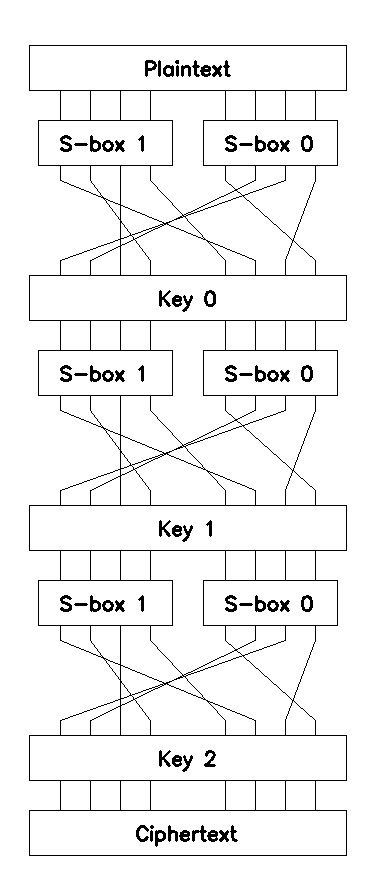
Let’s illustrate this idea by applying it to a toy three-round SP-network with \(8\)-bits block, P-box \(\mathcal{P}\), two \(4\)-bit input \(4\)-bit output S-boxes \(\mathcal{S}_0\), \(\mathcal{S}_1\), and three independent round keys \(\mathcal{K}_0..\mathcal{K}_2\):
Linear approximations of S-boxes
To find linear approximations with high absolute value of bias we generally apply a brute-force search in the space of all possible linear equations that relate inputs \(x_i\) to outputs \(y_j\).
To calculate bias \(\epsilon_k\) of a given linear equation \(l_k\) with input mask \(\Phi_k\) and output mask \(\phi_k\) we enumerate all input values \(x_i\), evaluate \(S\mathopen{}\left(x_i\right)\mathclose{}\) and count the number of times \(c_k\) the equation (1) holds. The ratio of \(c_k\) to the total number of input values \(x_i\) gives the bias of the linear approximation \(l_k\):
Therefore, to find all the linear equations with high absolute value of bias we essentially enumerate all input masks \(\Phi_k\) and all output masks \(\phi_k\), calculate bias \(\epsilon_k\) and save it in a list. Sorting this list by \(|\epsilon_k|\) gives us the linear approximations we’re looking for.
The complexity of the algorithm is determined by the number of the input bits, \(n\), and the number of the output bits, \(m\), of the S-box, and, clearly, is \(O\mathopen{}\left(2^{2n + m}\right)\mathclose{}\).
|
For a more detailed description of the algorithm refer to [6], Algorithm 9.2. |
Let’s assume that applying this algorithm to our toy example with two S-boxes \(\mathcal{S}_0\) and \(\mathcal{S}_1\) gives us the following equations.
| \(\Phi\) | \(\phi\) | \(c_k\) | \(\epsilon\) | Expression |
|---|---|---|---|---|
1 |
1 |
11 |
0.187 |
\(x_0 \oplus y_0 = 0\) |
2 |
2 |
10 |
0.125 |
\(x_1 \oplus y_1 = 0\) |
| \(\Phi\) | \(\phi\) | \(c_k\) | \(\epsilon\) | Expression |
|---|---|---|---|---|
4 |
6 |
12 |
0.250 |
\(x_2 \oplus y_2 \oplus y_1 = 0\) |
8 |
8 |
10 |
0.125 |
\(x_3 \oplus y_3 = 0\) |
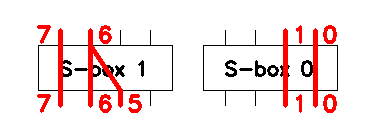
These linear equations for \(\mathcal{S}_0\) and \(\mathcal{S}_1\) can be used to build chained approximations that span through the whole cipher. The approximations are visualized in Figure 3.
Chaining approximations
Now that we’ve found some linear approximations we can trace outputs of the S-boxes through the P-box into the S-boxes on the next round and build chained approximations.
When linear cryptanalysis is applied to an SP-network, the chained approximations we actually need don’t go down to the ciphertext block \(c\), but span up to an S-box on the last round of encryption. These approximations provide us with a criterion for an exhaustive search for the last round key (see the next section Brute-forcing round key \(\mathcal{K}_2\)).
In the case of our toy example, the chained approximations we’re looking for relate the input bits of a plaintext block \(p\) to the input bits of the third round that we denote \(x^2_{0,3}..x^2_{0,0}\) and \(x^2_{1,3}..x^2_{1,0}\).
Concretely, let’s start with equation \(x_0 \oplus y_0 = 0\) of \(\mathcal{S}_0\) with bias \(\epsilon_0 = \frac{3}{16} \approx 0.187\). Applying this approximation on round \(0\) (the first round) we see that bit \(0\) of an input plaintext block, \(p_0\), is related to the output bit \(0\) of \(\mathcal{S}_0\), \(y^0_{0,0}\):
Tracing output \(0\) of \(\mathcal{S}_0\) on the first round through \(\mathcal{P}\) we see that \(y^0_{0,0}\) is XORed with \(k^0_1\) (bit \(1\) of the round key \(\mathcal{K}_0\)) and becomes \(x^1_{0,1}\) (input bit \(1\) of \(\mathcal{S}_0\) on round \(1\)):
Putting (2) in the equation above gives
Now let’s use the second approximation of \(\mathcal{S}_0\), \(x_1 \oplus y_1 = 0\), with \(\epsilon_1 = \frac{2}{16} = 0.125\), which for the second round can be rewritten as:
Tracing output \(1\) of \(\mathcal{S}_0\) on the second round through \(\mathcal{P}\) we see that \(y^1_{0,1}\) is XORed with \(k^1_7\) and becomes \(x^2_{1,3}\):
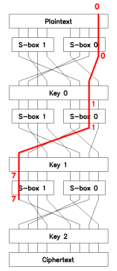
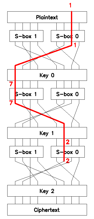
Equation (6) defines the first chained linear approximation, \(\mathcal{L}_1\), which can be used to brute-force \(4\) bits of the third round key \(\mathcal{K}_2\). \(\mathcal{L}_1\) is shown in Figure 4.
The bias of \(\mathcal{L}_1\) is given by Matsui’s Piling-up Lemma [3]:
which is a relatively significant value. The corresponding expected number of the known plaintext-ciphertext pairs required for the attack:
which is, again, a relatively reasonable amount of known pairs.
In a similar fashion, let’s build another chained approximation to relate inputs of \(\mathcal{S}_1\) on the last round to the bits of an input plaintext block \(p\).
To this end we:
-
rewrite \(x_1 \oplus y_1 = 0\) of \(\mathcal{S}_0\) on round \(0\) as
\[p_1 \oplus y^0_{0,1} = 0,\] -
trace \(y^0_{0,1}\) through \(\mathcal{P}\) to find
\[x^1_{1,3} = y^0_{0,1} \oplus k^0_7,\] -
rewrite \(x_3 \oplus y_3 = 0\) of \(\mathcal{S}_1\) on round \(1\) as
\[x^1_{1,3} \oplus y^1_{1,3} = 0,\] -
trace \(y^1_{1,3}\) through \(\mathcal{P}\) to find
\[x^2_{0,2} = y^1_{1,3} \oplus k^1_2.\]
Combining these, we obtain the second chained linear approximation, \(\mathcal{L}_2\):
which can be used to brute-force the other \(4\) bits of the third round key \(\mathcal{K}_2\). \(\mathcal{L}_2\) is shown in Figure 5.
The bias of \(\mathcal{L}_2\) is:
which is still an adequate value. The expected number of the known pairs is:
a tiny amount of known pairs as well.
Brute-forcing round key \(\mathcal{K}_2\)
The linear approximations \(\mathcal{L}_1\) and \(\mathcal{L}_2\) along with enough known plaintext-ciphertext pairs \(N_p\) allow us to find all \(8\) bits of the last round key \(\mathcal{K}_2\). Here we assume \(N_p > max\mathopen{}\left(N\mathopen{}\left(\mathcal{L}_1\right)\mathclose{}, N\mathopen{}\left(\mathcal{L}_2\right)\mathclose{}\right)\mathclose{}\).
Let’s use \(\mathcal{L}_1: x^2_{1,3} = p_0 \oplus k^0_1 \oplus k^1_7\) (equation (6)) to find \(4\) bits of \(\mathcal{K}_2\).
Note that \(x^2_{1,3}\) goes into \(\mathcal{S}_1\) on round \(2\) (see Figure 6). The outputs of \(\mathcal{S}_1\) are passed through \(\mathcal{P}\) and XORed with \(4\) bits of the last round key \(k^2_5, k^2_4, k^2_3, k^2_2\) to become \(4\) bits of the ciphertext block \(c_5, c_4, c_3, c_2\).
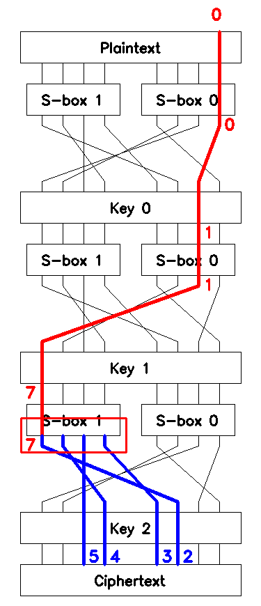
We assume that both \(p\) and \(c\) are known, so we can calculate
Obviously, \(4\) high bits of \(o\) are precisely the ciphertext bits in question: \(o_7 = c_2\), \(o_6 = c_4\), \(o_5 = c_5\), and \(o_4 = c_3\).
Let \(k_h = (k^2_2, k^2_4, k^2_5, k^2_3)\) and \(o_h = \mathopen{}\left(o_7,o_6,o_5,o_4\right)\mathclose{}\). Then, since \(\mathcal{S}_2\) is invertible (the toy cipher is an SP-network), we can find
Note that if \(k_h\) are the true key bits, then \(v_{h,3} = x^2_{1,3}\).
Here comes the key point: for the true key bits \(k_h\) we expect \(\mathcal{L}_1\) to hold with probability approximately \(Pr(\mathcal{L}_1) = 1/2 + \epsilon(\mathcal{L}_1)\), while for a random wrong key this probability should be closer to \(Pr(\mathcal{L}_1) = 1/2\).
This gives us a criterion for brute-force search: for a putative \(k_h\), estimate \(Pr(\mathcal{L}_1)\) using \(N_p\) known plaintext-ciphertext pairs, equations (8)-(9), and the linear approximation \(\mathcal{L}_1\). If \(Pr(\mathcal{L}_1)\) matches \(1/2 + \epsilon(\mathcal{L}_1)\) then \(k_h\) is likely to be the true key bits.
However, there’s a slight complication: generally, a linear approximation involves some key bits of the previous rounds, as is the case for \(\mathcal{L}_1\). To alleviate this problem, note that these key bits don’t depend on the bits \(k_h\) being enumerated, therefore their XOR is a constant value:
with \(a = const\), albeit unknown.
Hence, while evaluating the probability we actually check if
holds, completely ignoring the constant key bits \(a\). Then, depending on the value of \(a\):
-
if \(a = 0\), \(\mathcal{L}^{\prime}_1\) should hold with \(Pr(\mathcal{L}^{\prime}_1) = 1/2 + \epsilon(\mathcal{L}_1)\),
-
if \(a = 1\), \(\mathcal{L}^{\prime}_1\) should not hold with \(1/2 + \epsilon(\mathcal{L}_1)\), in other words, \(Pr(\mathcal{L}^{\prime}_1) = 1 - (1/2 + \epsilon(\mathcal{L}_1)) = 1/2 - \epsilon(\mathcal{L}_1)\).
Still, for a wrong \(k_h\) \(\mathcal{L}^{\prime}_1\) should hold with probability close to \(Pr(\mathcal{L}^{\prime}_1) = 1/2\).
Therefore, the quantity
can be used to distinguish the true key regardless of \(a\).
| Note that the absolute value is considered, so linear approximations with a negative bias values (i.e. such that hold rarely) can also be used in the analysis. One way to think about it is that along with the key bits of the previous rounds \(a\) "absorbs" the sign of the bias value as well. |
Which leads to the following algorithm for brute-force search for \(k_h\) key bits:
-
enumerate all the putative \(k_h\) values,
-
for each \(k_h\) set \(T_h = 0\) and enumerate all the \(N_p\) known pairs,
-
for each known pair:
-
finally, calculate \(f_h = |T_h/N_p - 1/2|\).
Sorting by \(f_h\) values in descending order we get a list of probable key values. Provided \(N_p\) is sufficient, we can take the first (the most probable) value as \(k_h\).
| Essentially, this is Matsui’s Algorithm 2 applied to an SP-network, see [3]. |
The complexity of the algorithm is largely determined by the number of bits being enumerated and is \(O\mathopen{}\left(2^{log\left(k_h\right)}\right)\mathclose{}\) for every chained linear expression considered.
To get the other \(4\) bits of the key \(\mathcal{K}_2\) we make use of the other linear approximation \(\mathcal{L}_2: x^2_{0,2} = p_1 \oplus k^0_7 \oplus k^1_2\) (equation (7)) and repeat the procedure described above.
Note that \(x^2_{0,2}\) goes into \(\mathcal{S}_0\) on round \(2\) (see Figure 7). The outputs of \(\mathcal{S}_0\) are passed through \(\mathcal{P}\) and XORed with the other \(4\) bits of the last round key \(k^2_7, k^2_6, k^2_1, k^2_0\) to become \(4\) bits of the ciphertext block \(c_7, c_6, c_1, c_0\).
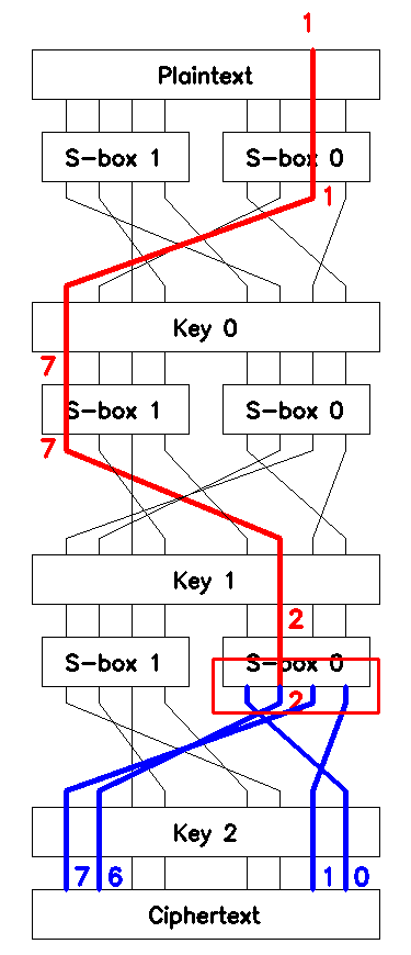
Using (8), we calculate \(o\). Let \(k_l = (k^2_0, k^2_6, k^2_7, k^2_1)\) and \(o_l = (o_0,o_6,o_7,o_1)\). Then (9) becomes
and, again, if \(k_l\) are the true key bits, then \(v_{l,2} = x^2_{0,2}\).
Then, similarly to (10), we define
and use the algorithm (with equations (11)-(12)) to brute-force the key bits and find the most probable value \(k_l\).
Finally, having found the two most probable halves, we simply concatenate \(k_h\) and \(k_l\) and pass the concatenation through \(\mathcal{P}\) to get the last round key:
Finding round keys \(\mathcal{K}_1\) and \(\mathcal{K}_0\)
Now that \(\mathcal{K}_2\) is known, we can decrypt the last round of encryption for all the known ciphertext blocks. Since the S-boxes and the P-box don’t change from round to round, our task now is to analyse two-round version of the toy cipher in the same KPA setting.
Conveniently, we can trim the beginnings of \(\mathcal{L}_1\) and \(\mathcal{L}_2\) and apply these trimmed approximations to perform brute-force search for the bits of the round key \(\mathcal{K}_1\). One way to think about it is that these chained approximations are moved one round up with the exceeded equations removed, see Figure 8.
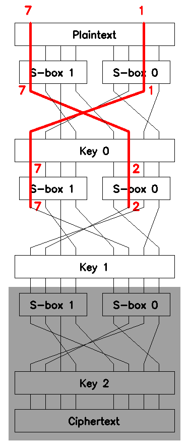
Essentially, the only relevant change is the plaintext bits that we use in the trimmed linear approximations: \(\mathcal{L}_1\) becomes
and \(\mathcal{L}_2\) is now
Therefore, to get \(\mathcal{K}_1\) we repeat the algorithm for brute-force search, replacing \(p_0\) with \(p_1\) for \(\mathcal{L}_1\) and \(p_1\) with \(p_7\) for \(\mathcal{L}_2\).
Having found the most probable \(\mathcal{K}_1\) we decrypt one more round of encryption and the task becomes breaking one-round SP-network, which actually doesn’t require applying linear cryptanalysis as the key \(\mathcal{K}_0\) can be calculated directly:
where \(r = D_{\mathcal{K}_1}(D_{\mathcal{K}_2}(c))\) is partially decrypted ciphertext block \(c\).
Finally, with all the round keys known we can decrypt any ciphertext, so the toy cipher is broken!
3. Searching for linear approximations
Now that we’ve identified the likely weakness of the cipher SPlin, let’s proceed with finding linear approximations of S-boxes \(S_0..S_7\) with significant bias values.
The following code snippet taken from the solution script solution.py implements the exhaustive search for linear approximations described in section Linear approximations of S-boxes and executes it for each S-box \(S_0..S_7\):
24
25
26
27
28
29
30
31
32
33
34
35
36
37
38
39
40
41
42
43
44
45
def find_approximations_sbox(sbox):
    length = len(sbox)
    approximations = []

    # 1. calculate the biases for all the possible approximations
    for mask_in in range(length):                                                    (1)
        for mask_out in range(length):                                               (1)
            count = 0
            for x in range(length):                                                  (1)
                if scalar_product(x, mask_in) == scalar_product(sbox[x], mask_out):  (2)
                    count += 1
            approximations.append({
                'mask_in': mask_in,
                'mask_out': mask_out,
                'count': count,
                'bias': count / length - 0.5,                                        (3)
                'p': count / length
            })

    # 2. sort by counts and return
    approximations = sorted(approximations, key=lambda _x: abs(_x['bias']), reverse=True)
    return approximations
| 1 | Enumerate input masks \(\Phi\), output masks \(\phi\), and inputs \(x\). |
| 2 | Check (1) to see if the linear approximation defined by \(\Phi\) and \(\phi\) holds. |
| 3 | Calculate an estimate of the linear approximation’s bias. |
66
67
68
69
70
def find_approximations():
    for i, sbox in enumerate([SBOX0, SBOX1, SBOX2, SBOX3, SBOX4, SBOX5, SBOX6, SBOX7]):
        print('Linear approximations of SBOX%d' % i)
        output_approximations(find_approximations_sbox(sbox), n_appr=8)
        print('\n')
For each S-box function find_approximations outputs \(t = 8\) linear equations with the highest absolute value of bias:
Linear approximations of SBOX0
  in  out  count   p     bias    expr
   0    0  256   1.000   0.500   0 = 0
  70   b7   94   0.367  -0.133   x6 + x5 + x4 = y7 + y5 + y4 + y2 + y1 + y0
  f3   b6  162   0.633   0.133   x7 + x6 + x5 + x4 + x1 + x0 = y7 + y5 + y4 + y2 + y1
   4   c0  160   0.625   0.125   x2 = y7 + y6
  20   67  160   0.625   0.125   x5 = y6 + y5 + y2 + y1 + y0
  35   12   96   0.375  -0.125   x5 + x4 + x2 + x0 = y4 + y1
  48   21  160   0.625   0.125   x6 + x3 = y5 + y0
  59   d2   96   0.375  -0.125   x6 + x4 + x3 + x0 = y7 + y6 + y4 + y1


Linear approximations of SBOX1
  in  out  count   p     bias    expr
   0    0  256   1.000   0.500   0 = 0
   1   60  168   0.656   0.156   x0 = y6 + y5
...
The output is summarized in the following tables. Note that uninformative \(x_0 = y_0\) with bias \(0.5\) is not included since it’s useless. Also, the maximum count value \(c_k\) is \(2^8 = 256\).
| \(\Phi\) | \(\phi\) | \(c_k\) | \(\epsilon\) | Expression |
|---|---|---|---|---|
70 |
b7 |
94 |
-0.133 |
\(x_6 \oplus x_5 \oplus x_4 = y_7 \oplus y_5 \oplus y_4 \oplus y_2 \oplus y_1 \oplus y_0\) |
f3 |
b6 |
162 |
0.133 |
\(x_7 \oplus x_6 \oplus x_5 \oplus x_4 \oplus x_1 \oplus x_0 = y_7 \oplus y_5 \oplus y_4 \oplus y_2 \oplus y_1\) |
4 |
c0 |
160 |
0.125 |
\(x_2 = y_7 \oplus y_6\) |
20 |
67 |
160 |
0.125 |
\(x_5 = y_6 \oplus y_5 \oplus y_2 \oplus y_1 \oplus y_0\) |
35 |
12 |
96 |
-0.125 |
\(x_5 \oplus x_4 \oplus x_2 \oplus x_0 = y_4 \oplus y_1\) |
48 |
21 |
160 |
0.125 |
\(x_6 \oplus x_3 = y_5 \oplus y_0\) |
59 |
d2 |
96 |
-0.125 |
\(x_6 \oplus x_4 \oplus x_3 \oplus x_0 = y_7 \oplus y_6 \oplus y_4 \oplus y_1\) |
| \(\Phi\) | \(\phi\) | \(c_k\) | \(\epsilon\) | Expression |
|---|---|---|---|---|
1 |
60 |
168 |
0.156 |
\(x_0 = y_6 \oplus y_5\) |
5a |
c2 |
164 |
0.141 |
\(x_6 \oplus x_4 \oplus x_3 = y_7 \oplus y_6 \oplus y_1\) |
e |
97 |
96 |
-0.125 |
\(x_3 \oplus x_2 \oplus x_1 = y_7 \oplus y_4 \oplus y_2 \oplus y_1 \oplus y_0\) |
18 |
e8 |
96 |
-0.125 |
\(x_4 \oplus x_3 = y_7 \oplus y_6 \oplus y_5 \oplus y_3\) |
20 |
20 |
160 |
0.125 |
\(x_5 = y_5\) |
34 |
80 |
160 |
0.125 |
\(x_5 \oplus x_4 \oplus x_2 = y_7\) |
59 |
f |
160 |
0.125 |
\(x_6 \oplus x_4 \oplus x_3 \oplus x_0 = y_3 \oplus y_2 \oplus y_1 \oplus y_0\) |
| \(\Phi\) | \(\phi\) | \(c_k\) | \(\epsilon\) | Expression |
|---|---|---|---|---|
81 |
3 |
252 |
0.484 |
\(x_7 \oplus x_0 = y_1 \oplus y_0\) |
91 |
2b |
252 |
0.484 |
\(x_7 \oplus x_4 \oplus x_0 = y_5 \oplus y_3 \oplus y_1 \oplus y_0\) |
1 |
1 |
248 |
0.469 |
\(x_0 = y_0\) |
10 |
28 |
248 |
0.469 |
\(x_4 = y_5 \oplus y_3\) |
80 |
2 |
248 |
0.469 |
\(x_7 = y_1\) |
11 |
29 |
244 |
0.453 |
\(x_4 \oplus x_0 = y_5 \oplus y_3 \oplus y_0\) |
90 |
2a |
244 |
0.453 |
\(x_7 \oplus x_4 = y_5 \oplus y_3 \oplus y_1\) |
| \(\Phi\) | \(\phi\) | \(c_k\) | \(\epsilon\) | Expression |
|---|---|---|---|---|
8 |
2 |
252 |
0.484 |
\(x_3 = y_1\) |
51 |
50 |
252 |
0.484 |
\(x_6 \oplus x_4 \oplus x_0 = y_6 \oplus y_4\) |
59 |
52 |
252 |
0.484 |
\(x_6 \oplus x_4 \oplus x_3 \oplus x_0 = y_6 \oplus y_4 \oplus y_1\) |
58 |
12 |
248 |
0.469 |
\(x_6 \oplus x_4 \oplus x_3 = y_4 \oplus y_1\) |
1 |
40 |
244 |
0.453 |
\(x_0 = y_6\) |
9 |
42 |
244 |
0.453 |
\(x_3 \oplus x_0 = y_6 \oplus y_1\) |
50 |
10 |
244 |
0.453 |
\(x_6 \oplus x_4 = y_4\) |
| \(\Phi\) | \(\phi\) | \(c_k\) | \(\epsilon\) | Expression |
|---|---|---|---|---|
9 |
90 |
92 |
-0.141 |
\(x_3 \oplus x_0 = y_7 \oplus y_4\) |
d |
41 |
164 |
0.141 |
\(x_3 \oplus x_2 \oplus x_0 = y_6 \oplus y_0\) |
4 |
18 |
160 |
0.125 |
\(x_2 = y_4 \oplus y_3\) |
39 |
a9 |
160 |
0.125 |
\(x_5 \oplus x_4 \oplus x_3 \oplus x_0 = y_7 \oplus y_5 \oplus y_3 \oplus y_0\) |
3e |
9 |
160 |
0.125 |
\(x_5 \oplus x_4 \oplus x_3 \oplus x_2 \oplus x_1 = y_3 \oplus y_0\) |
83 |
68 |
160 |
0.125 |
\(x_7 \oplus x_1 \oplus x_0 = y_6 \oplus y_5 \oplus y_3\) |
85 |
f8 |
160 |
0.125 |
\(x_7 \oplus x_2 \oplus x_0 = y_7 \oplus y_6 \oplus y_5 \oplus y_4 \oplus y_3\) |
| \(\Phi\) | \(\phi\) | \(c_k\) | \(\epsilon\) | Expression |
|---|---|---|---|---|
81 |
11 |
242 |
0.445 |
\(x_7 \oplus x_0 = y_4 \oplus y_0\) |
85 |
19 |
242 |
0.445 |
\(x_7 \oplus x_2 \oplus x_0 = y_4 \oplus y_3 \oplus y_0\) |
4 |
8 |
240 |
0.438 |
\(x_2 = y_3\) |
84 |
9 |
240 |
0.438 |
\(x_7 \oplus x_2 = y_3 \oplus y_0\) |
1 |
10 |
238 |
0.430 |
\(x_0 = y_4\) |
5 |
18 |
238 |
0.430 |
\(x_2 \oplus x_0 = y_4 \oplus y_3\) |
80 |
1 |
232 |
0.406 |
\(x_7 = y_0\) |
| \(\Phi\) | \(\phi\) | \(c_k\) | \(\epsilon\) | Expression |
|---|---|---|---|---|
8 |
1 |
250 |
0.477 |
\(x_3 = y_0\) |
40 |
10 |
250 |
0.477 |
\(x_6 = y_4\) |
41 |
30 |
248 |
0.469 |
\(x_6 \oplus x_0 = y_5 \oplus y_4\) |
48 |
11 |
248 |
0.469 |
\(x_6 \oplus x_3 = y_4 \oplus y_0\) |
1 |
20 |
246 |
0.461 |
\(x_0 = y_5\) |
9 |
21 |
244 |
0.453 |
\(x_3 \oplus x_0 = y_5 \oplus y_0\) |
49 |
31 |
242 |
0.445 |
\(x_6 \oplus x_3 \oplus x_0 = y_5 \oplus y_4 \oplus y_0\) |
| \(\Phi\) | \(\phi\) | \(c_k\) | \(\epsilon\) | Expression |
|---|---|---|---|---|
ca |
4a |
92 |
-0.141 |
\(x_7 \oplus x_6 \oplus x_3 \oplus x_1 = y_6 \oplus y_3 \oplus y_1\) |
20 |
c |
160 |
0.125 |
\(x_5 = y_3 \oplus y_2\) |
43 |
d1 |
96 |
-0.125 |
\(x_6 \oplus x_1 \oplus x_0 = y_7 \oplus y_6 \oplus y_4 \oplus y_0\) |
65 |
16 |
96 |
-0.125 |
\(x_6 \oplus x_5 \oplus x_2 \oplus x_0 = y_4 \oplus y_2 \oplus y_1\) |
95 |
c2 |
96 |
-0.125 |
\(x_7 \oplus x_4 \oplus x_2 \oplus x_0 = y_7 \oplus y_6 \oplus y_1\) |
bb |
6c |
160 |
0.125 |
\(x_7 \oplus x_5 \oplus x_4 \oplus x_3 \oplus x_1 \oplus x_0 = y_6 \oplus y_5 \oplus y_3 \oplus y_2\) |
ef |
ef |
96 |
-0.125 |
\(x_7 \oplus x_6 \oplus x_5 \oplus x_3 \oplus x_2 \oplus x_1 \oplus x_0 = y_7 \oplus y_6 \oplus y_5 \oplus y_3 \oplus y_2 \oplus y_1 \oplus y_0\) |
| The linear equations that will be used later are shown in bold. |
The total complexity of the search is \(O\mathopen{}\left(2^{27}\right)\mathclose{}\), as we applied the brute-force search to an \(8\)-bit input \(8\)-output S-box \(8\) times.
As can be seen, a lot of linear equations have high absolute value of bias. Some shown approximations may occur at random, for their bias values, albeit relatively large, are still adequate. The other equations (with bias exceeding \(0.4\)) are almost certainly artificial.
4. Chaining approximations up to the last round
The next step is to build chained linear approximations that span through the first three rounds of encryption. Such approximations can be used in brute-force search for the last round key \(K_3\).
Essentially, we follow the procedure described in Chaining approximations.
| As to how we note which equations can be chained together, the answer is: "eyeballing". However, in theory this process can be automated, the interested reader is referred to [7]. |
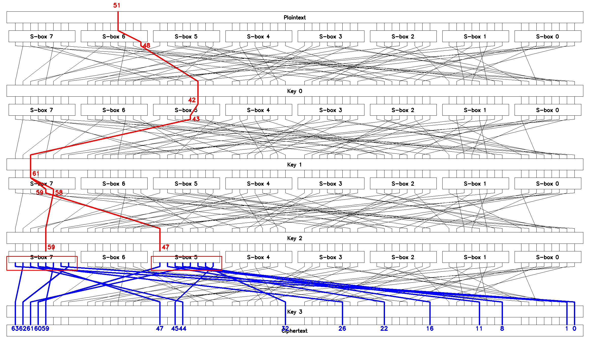
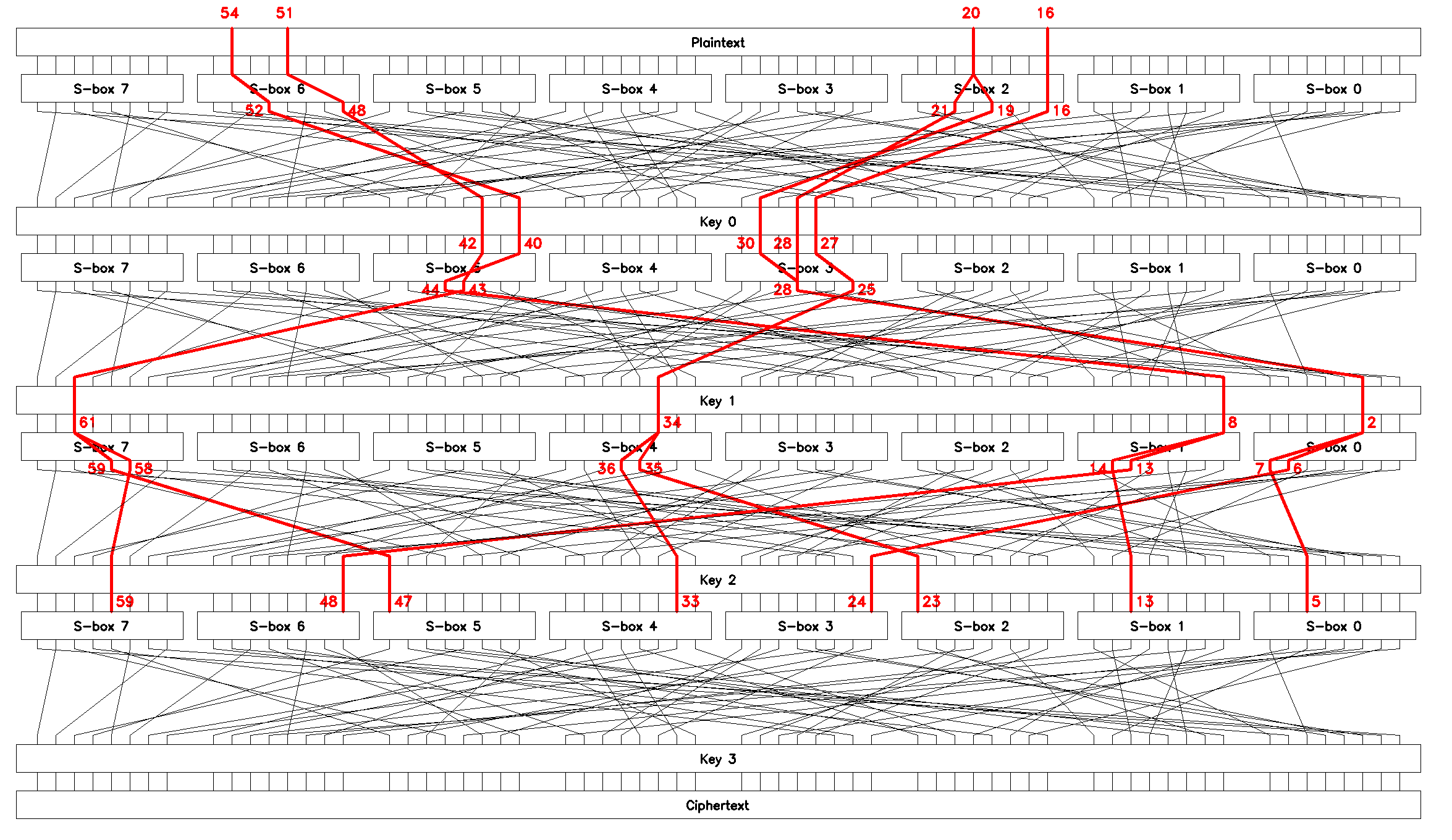
Linear approximation \(L_1\)
Let’s build an approximation that relates inputs of \(S_1\) and \(S_6\) on the last round to the bits of an input plaintext block \(p\).
| In the following we’ll be using two types of indexing: "local" and "global", e.g. \(x^1_{4,2}\) and \(x^1_{34}\), respectively. Both \(x^1_{4,2}\) and \(x^1_{34}\) signify the same bit since the S-boxes are \(8\)-bit input \(8\)-bit output and \(4 \cdot 8 + 2 = 34\). Notation is defined in section Definitions. |
The process comprises the following steps:
-
rewrite \(x_6 \oplus y_4 = 0\) of \(S_6\) (Table 9) on round \(0\) with \(\epsilon_1 = 0.477\) as
\[x^0_{6,6} \oplus y^0_{6,4} = p_{54} \oplus y^0_{52} = 0,\] -
trace \(y^0_{52}\) through \(P\) to find
\[x^1_{40} = x^1_{5,0} = y^0_{52} \oplus k^0_{40},\] -
rewrite \(x_0 \oplus y_4 = 0\) of \(S_5\) (Table 8) on round \(1\) with \(\epsilon_2 = 0.430\) as
\[x^1_{5,0} \oplus y^1_{5,4} = x^1_{40} \oplus y^1_{44} = 0,\] -
trace \(y^1_{44}\) through \(P\) to find
\[x^2_8 = x^2_{1,0} = y^1_{44} \oplus k^1_8.\] -
rewrite \(x_0 \oplus y_6 \oplus y_5 = 0\) of \(S_1\) (Table 4) on round \(2\) with \(\epsilon_3 = 0.156\) as
\[x^2_{1,0} \oplus y^2_{1,6} \oplus y^2_{1,5} = x^2_8 \oplus y^2_{14} \oplus y^2_{13} = 0,\] -
finally, trace \(y^2_{14}\) and \(y^2_{13}\) through \(P\) to obtain
\[\begin{split} x^3_{48} = x^3_{6,0} = y^2_{13} \oplus k^2_{48}, \\ x^3_{13} = x^3_{1,5} = y^2_{14} \oplus k^2_{13}. \end{split}\]
Combining these, we get
Rearranging
we drop the unknown but constant key bits on the right (as discussed in section Brute-forcing round key \(\mathcal{K}_2\)) to obtain the first chained linear approximation, \(L_1\):
which can be used to brute-force two bytes \(1\) and \(6\) of the last round key \(K_3\). \(L_1\) is shown in Figure 9.
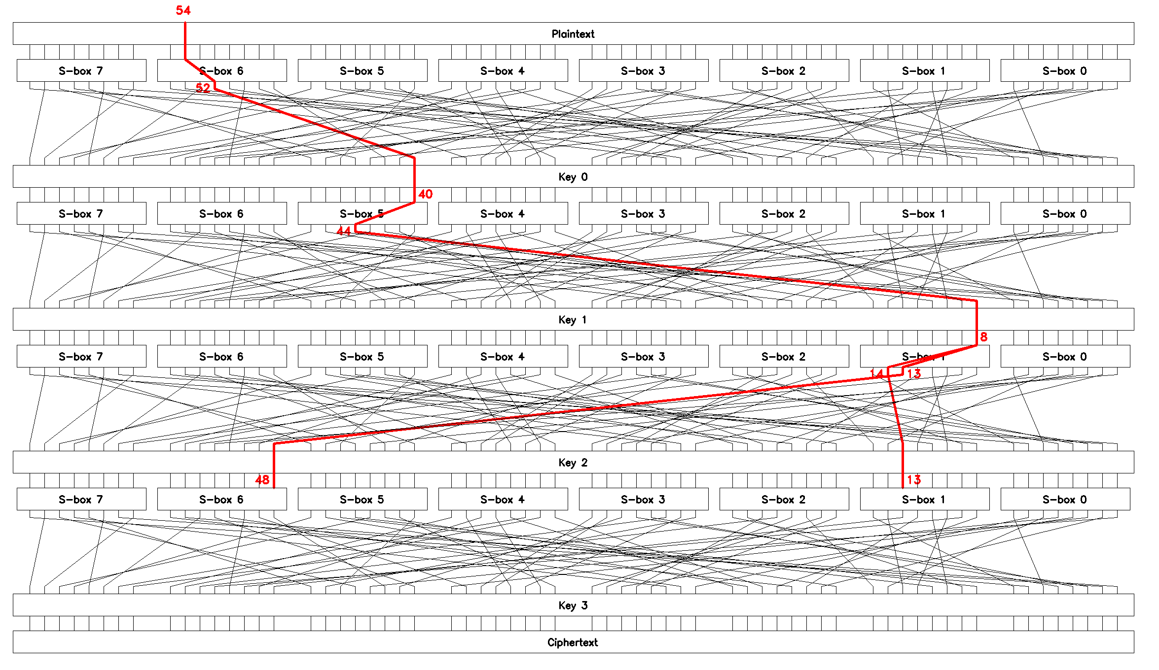
SPlinApplying Matsui’s Piling-up Lemma [3], we find the bias of \(L_1\):
which is a huge value. The expected number of the known plaintext-ciphertext pairs is:
a tiny amount compared to \(N_p = 35145\) known pairs we are given (see Recon results).
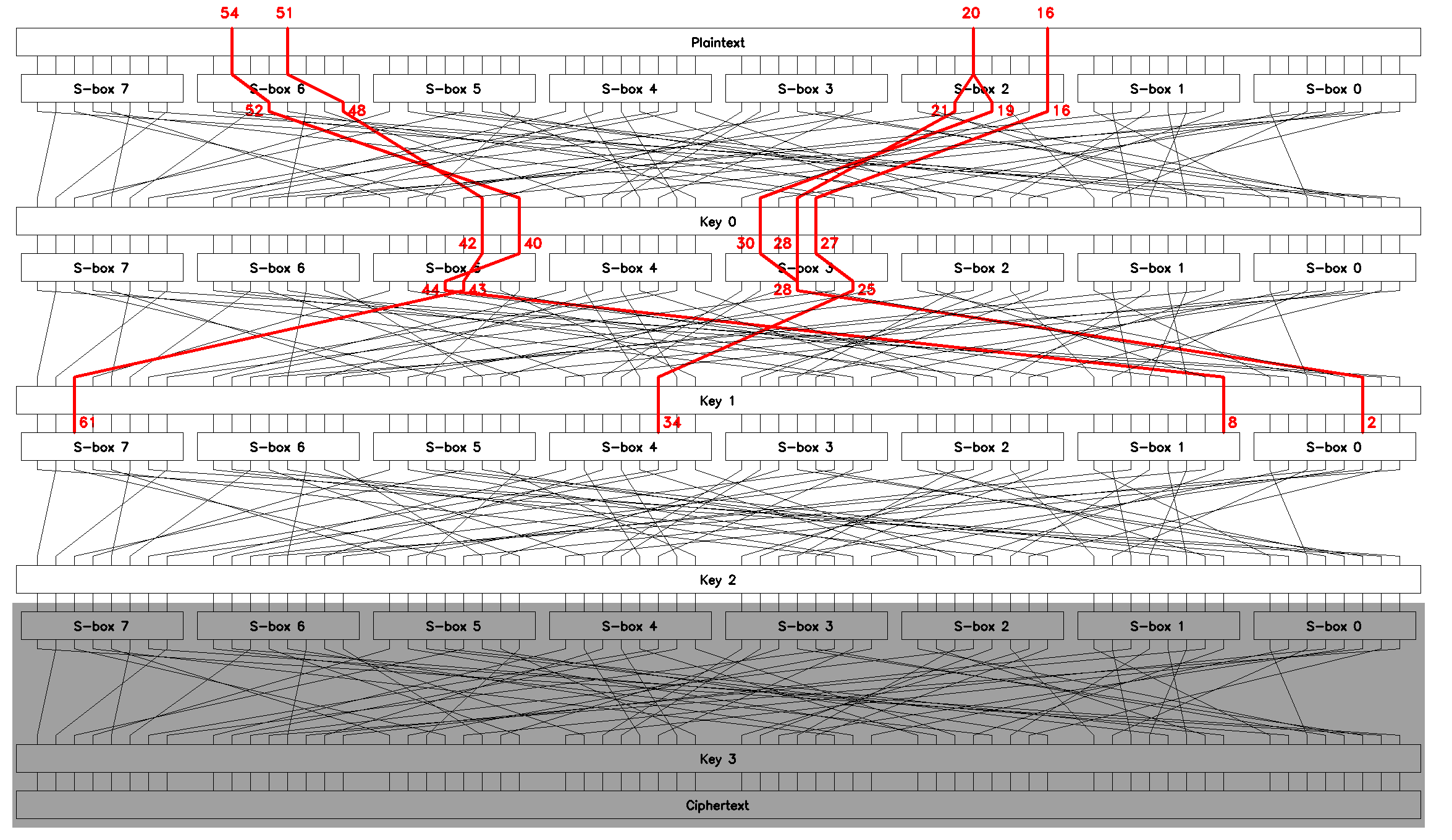
Linear approximation \(L_2\)
Following the same route we build an approximation that relates inputs of \(S_5\) and \(S_7\) on the last round to the bits of an input plaintext block \(p\).
To this end note:
-
\(x_3 \oplus y_0 = p_{51} \oplus y^0_{48} = 0\) of \(S_6\) (Table 9) on round \(0\) with \(\epsilon_1 = 0.477\),
-
\(P\) maps bit \(48\) to bit \(42\),
-
\(x_2 \oplus y_3 = x^1_{42} \oplus y^1_{43} = 0\) of \(S_5\) (Table 8) on round \(1\) with \(\epsilon_2 = 0.438\),
-
\(P\) maps \(43\) to \(61\),
-
\(x_5 \oplus y_3 \oplus y_2 = x^2_{61} \oplus y^2_{59} \oplus y^2_{58} = 0\) of \(S_7\) (Table 10) on round \(2\) with \(\epsilon_3 = 0.125\),
-
\(P\) maps \(58\) to \(59\) and \(59\) to \(47\).
Combining, we find
Rearranging and dropping the unknown but constant key bits we obtain the second chained linear approximation, \(L_2\):
which can be used to brute-force bytes \(5\) and \(7\) of the last round key \(K_3\). \(L_2\) is shown in Figure 10.
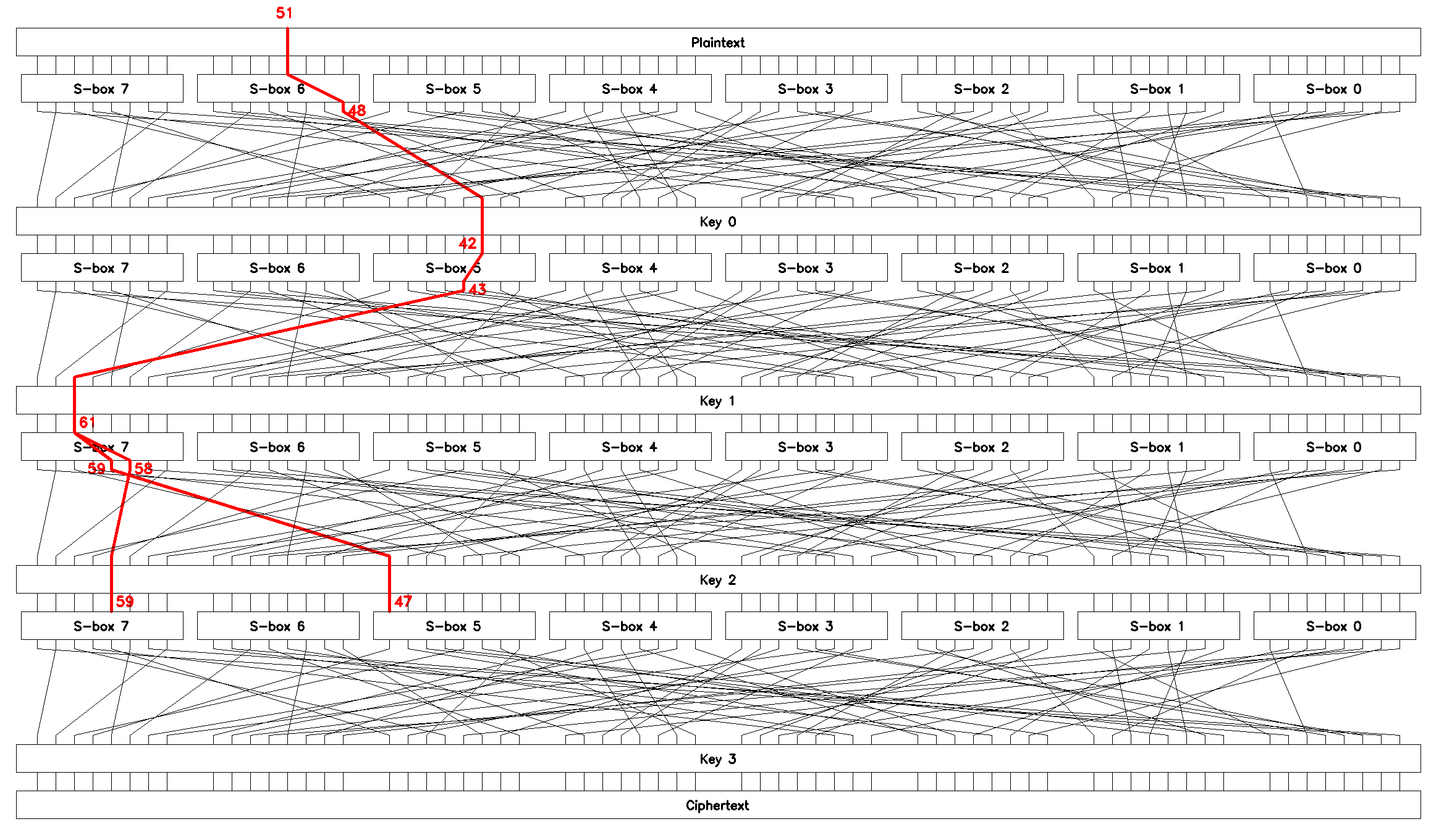
SPlinThe bias of \(L_2\) is:
a significant value. The expected number of the known plaintext-ciphertext pairs is:
which is also negligible compared to \(N_p = 35145\) known pairs.
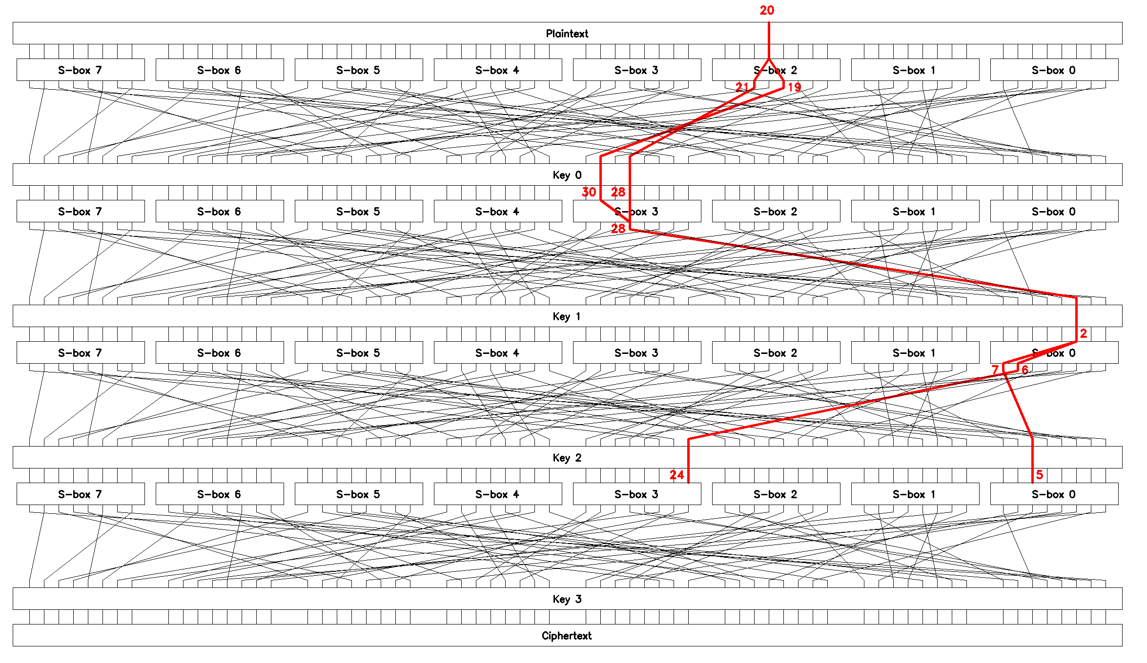
Linear approximations \(L_3\) and \(L_4\)
The reader is encouraged to repeat the procedure described in the previous sections to come up with chained linear approximations that relate inputs of \(S_0\), \(S_2\), \(S_3\), and \(S_5\) to the bits of an input plaintext block \(p\). The approximations we’re going to use later in the brute-force attack are described below.
The third chained linear approximation, \(L_3\):
can be used to brute-force bytes \(0\) and \(3\) of the last round key \(K_3\).
The bias of the equation \(\epsilon(L_3) \approx 0.106\), the expected number of known plaintext-ciphertext pairs \(N(L_3) \approx 709\). \(L_3\) is shown in Figure 11.
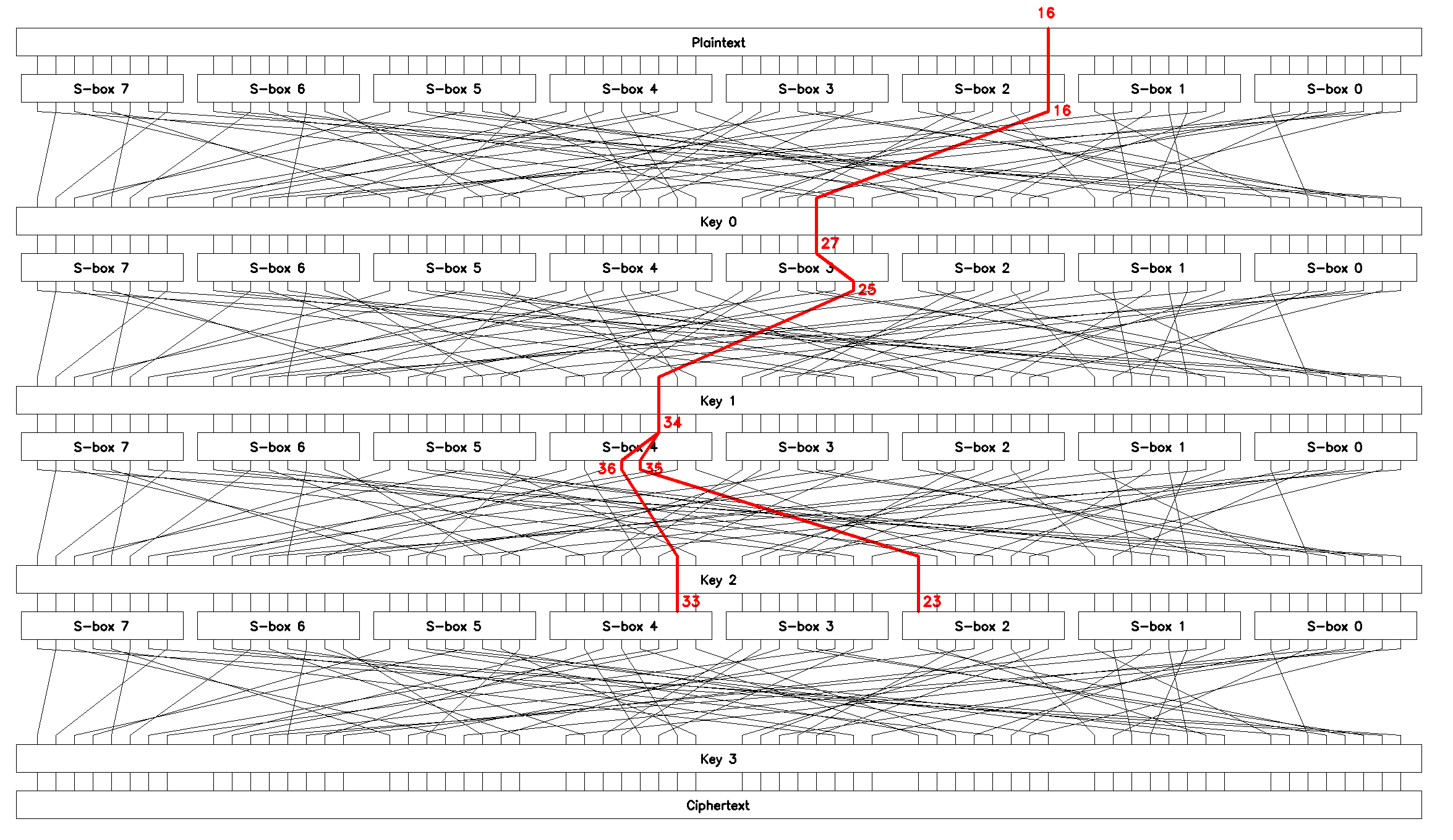
SPlinThe fourth chained linear approximation, \(L_4\):
can be used to brute-force bytes \(2\) and \(4\) of the last round key \(K_3\).
The bias of the equation \(\epsilon(L_4) \approx 0.113\), the expected number of known plaintext-ciphertext pairs \(N(L_4) \approx 621\). \(L_4\) is shown in Figure 12.
SPlin|
Chaining the linear approximations of the S-boxes \(S_0..S_7\) we found:
|
5. Brute-forcing the last round key \(K_3\)
Having found four chained linear approximations \(L_1..L_4\) that span through the first three rounds of encryption we are ready to perform brute-force search for putative round key \(K_3\) values.
First we need to prepare known plaintext-ciphertext pairs, then brute-force four subkeys - two-byte parts of \(K_3\), and, finally, join the subkeys to get the most probable round key. We discuss every step in detail in the following sections.
Preparing the data
Preparing known plaintext-ciphertext block pairs is easy and is implemented in function read_plaintext_ciphertext_pairs from the solution script solution.py.
Essentially, it amounts to the following steps:
-
read the ciphertext bytes from
test.bin.enc, -
regenerate the missing plaintext bytes using the known PRNG seed value (see check_encryption_file),
-
split byte-arrays into lists of \(8\)-byte integers,
-
redo CBC chaining of the plaintext blocks.
The last step deserves explanation. Analysis of SPlin cipher showed (Cipher implementation region) that all the plaintext data, including the data corresponding to the given file test.bin.enc, are encrypted in CBC-mode. This means that prior to being encrypted every plaintext block is XORed with the previous ciphertext block (see [2]).
Therefore, to get the actual plaintext-ciphertext pairs we need to repeat this process for the regenerated plaintext blocks, as done in this snippet taken from read_plaintext_ciphertext_pairs:
181
182
183
184
    # 4. IMPORTANT: redo CBC to get the actual plaintext-ciphertext pairs
    for i in range(len(pbs)):
        pbs[i] ^= cbs[i]        (1)
    cbs = cbs[1:]               (2)
| 1 | CBC redoing |
| 2 | Obviously, cbs[0] is the IV, so it must be removed. |
Brute-forcing subkeys
Here comes the core part of the brute-force search. This is almost exactly the brute-force search algorithm described in section Brute-forcing round key \(\mathcal{K}_2\).
This procedure is implemented as function _attack_subkey_part in solution.py:
77
78
79
80
81
82
83
84
85
86
87
88
89
90
91
92
93
94
95
96
97
98
def _attack_subkey_part(mask_p, mask_c, subkey_parts_indices, pbs, cbs):
    # 1. enumerate all the possible subkey parts and calculate the likelihoods
    n_known_pairs = len(pbs)
    putative_keys = []
    for kb in product(range(256), repeat=len(subkey_parts_indices)):            (1)
        # make the next putative subkey part
        key = 0
        for b, sh in zip(kb, subkey_parts_indices):                             (2)
            key |= b << (8 * sh)

        #  calculate the number of times the given linear equation holds
        count = 0
        for pb, cb in zip(pbs, cbs):
            if scalar_product(pb, mask_p) == \                                  (3)
                    scalar_product(sboxes_inv(pbox_inv(cb) ^ key), mask_c):     (4)
                count += 1

        putative_keys.append((count, key, abs(count - n_known_pairs // 2)))     (5)

    # 2. sort by |count - N/2| in descending order
    putative_keys = sorted(putative_keys, key=lambda _x: _x[2], reverse=True)   (6)
    return putative_keys
| 1 | Enumerate len(subkey_parts_indices) * 8 bits of the key. |
| 2 | Place the subkey bytes at indices given in the subkey_parts_indices |
| 3 | Evaluate the chained linear approximation defined by the input mask mask_p and the output mask mask_c. Note that the representation (1) is used. |
| 4 | Ciphertext block cb is passed back through the P-box, XORed with the subkey, and passed through the inverted S-boxes. This line evaluates (8)-(9). |
| 5 | For each subkey find \(v = |count - N/2|\), which is essentially an estimate of the linear approximation’s absolute value of bias times the number of known pairs \(N\). |
| 6 | Sort putative subkeys by this value \(v\) to get the most probable keys. |
|
This is an exceptionally slow version. Disastrously slow. The reader is challenged to speed it up, e.g. by using For example, |
Note that in order to operate on byte level while performing brute-force search we pass ciphertext block \(c\) through \(P^{-1}\) and XOR with the next subkey "right before" the S-boxes, see Figure 13. This allows us to simplify the code. What’s left is to pass the found key through \(P\) to get the actual round key (see the next section, Attack round key \(K_3\)).
While not negligible, the complexity of the inner loop that evaluates (1) for every known plaintext-ciphertext pair is constant and linear in the number of pairs \(N_p\). Therefore, we can claim that the complexity of this algorithm is \(O\mathopen{}\left(2^{n_b}\right)\mathclose{}\), where \(n_b\) is the number of the key bits being searched for (len(subkey_parts_indices) * 8 in the code above).
When this algorithm is finally over, we get a list of len(subkey_parts_indices)-bytes subkeys of \(K_3\) that are likely to be the correct one.
Attack round key \(K_3\)
At this point we are ready to search for the last round key \(K_3\), repeatedly passing the correct arguments to _attack_subkey_part. That is, we need to represent a chained linear approximation as a set of input and output masks, and describe the corresponding two-byte subkey as a set of indices.
This procedure is implemented in function attack_round_three:
116
117
118
119
120
121
122
123
124
125
126
def attack_round_three(pbs, cbs, n_keys=3):
    print('ROUND 3')
    putative_keys_16 = attack_subkey_part(1 << 54, (1 << 48) | (1 << 13), [1, 6], pbs, cbs, stage=1, n_keys=n_keys)    (1)
    putative_keys_57 = attack_subkey_part(1 << 51, (1 << 59) | (1 << 47), [5, 7], pbs, cbs, stage=2, n_keys=n_keys)    (2)
    putative_keys_03 = attack_subkey_part(1 << 20, (1 << 24) | (1 << 5), [0, 3], pbs, cbs, stage=3, n_keys=n_keys)    (2)
    putative_keys_24 = attack_subkey_part(1 << 16, (1 << 33) | (1 << 23), [2, 4], pbs, cbs, stage=4, n_keys=n_keys)    (2)

    round_key = pbox(putative_keys_16[0][1] | putative_keys_57[0][1] | putative_keys_03[0][1] | putative_keys_24[0][1])    (3)
    print('Found key[3] = %016lx' % round_key)

    return round_key
| 1 | \(L_1\): \(p_{54} = x^3_{48} \oplus x^3_{13}\) is represented by input mask \(\Phi_1 = \mathrm{0x0040000000000000}\) and output mask \(\phi_1 = \mathrm{0x0001000000002000}\), the corresponding bytes to be searched for are \(1\) and \(6\). |
| 2 | sim. for the other three approximations. |
| 3 | Optimistically, only the most probable subkeys are joined together and passed through \(P\) to get \(K_3\). |
This algorithm is run \(4\) times for \(16\)-bits subkeys, so the total complexity of round key search is \(O\mathopen{}\left(2^{18}\right)\mathclose{}\).
Running attack_round_three should give us \(K_3 = \mathrm{0x3564ea65bcbd493e}\), which is the correct last round key.
|
Brute-forcing the round key \(K_3\) using the chained linear approximations \(L_1..L_4\) we found \(K_3 = \mathrm{0x3564ea65bcbd493e}\). |
6. Brute-forcing round keys \(K_2\) and \(K_1\)
Having found \(K_3\), we can decrypt the last round of encryption for all the known ciphertext blocks. As the S-boxes \(S_0..S_7\) and the P-box \(P\) don’t change from round to round, our task now is to analyse three-round version of cipher SPlin in the KPA setting.
Generally, we follow the steps described in Finding round keys \(\mathcal{K}_1\) and \(\mathcal{K}_0\).
Searching for round key \(K_2\)
To define a criterion for brute-force search for \(K_2\) we can reuse the approximations \(L_1..L_4\) in two ways:
-
Trim the third linear equation from each of \(L_1..L_4\) to obtain chained approximations that relate inputs of \(S_0\), \(S_1\), \(S_4\), and \(S_7\) on round \(2\) to the bits of a plaintext block \(p\), see Figure 14. Using these equations we can find \(4\) bytes of the round key \(K_2\) for \(O\mathopen{}\left(2^{10}\right)\mathclose{}\).
-
Trim the first linear equation from each of \(L_1..L_4\) to "move" them up, Figure 15. This poses essentially the same brute-force search problem as was solved for \(K_3\), the only difference being the bits of \(p\) that are involved in the updated approximations.
The second approach gives us all \(8\) bytes of the key for a total of \(O\mathopen{}\left(2^{18}\right)\mathclose{}\) operations.
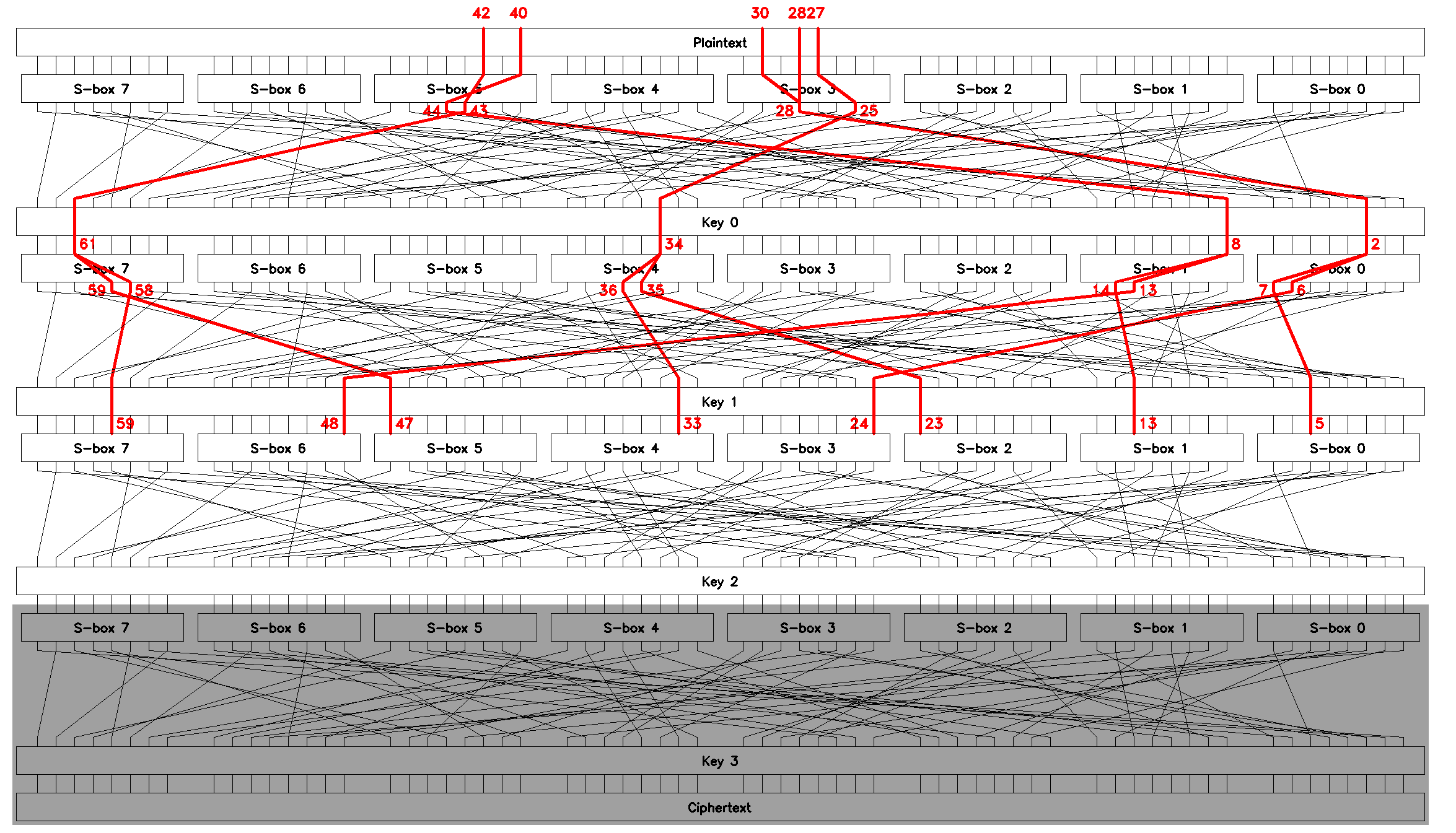
|
Actually, the two can be combined to gain more information about the correct key. Since every one-byte subkey found using the first approach is a half of a two-bytes subkey given by the second approach, we can take the most probable one-byte subkeys into account while ranking and selecting the most probable two-byte subkeys. Concretely, if the most probable two-byte subkey overlaps with the corresponding most probable one-byte subkey, this increases the probability of the former (actually, the both) being the true key parts. For this we only have to spend additional \(O\mathopen{}\left(2^{10}\right)\mathclose{}\), which is small a complexity compared to \(O\mathopen{}\left(2^{18}\right)\mathclose{}\). |
If we follow the second approach we can reuse the function _attack_subkey_part and only need to make tiny changes to function attack_round_three.
Searching for round key \(K_1\)
With the most probable \(K_2\) we decrypt the second-to-last round of encryption for all the partially decrypted ciphertext blocks.
Following the same route we "move" the two-round chained approximations up one round to get the equations that relate inputs of the S-boxes on round \(1\) to the bits of a plaintext block \(p\), Figure 16.
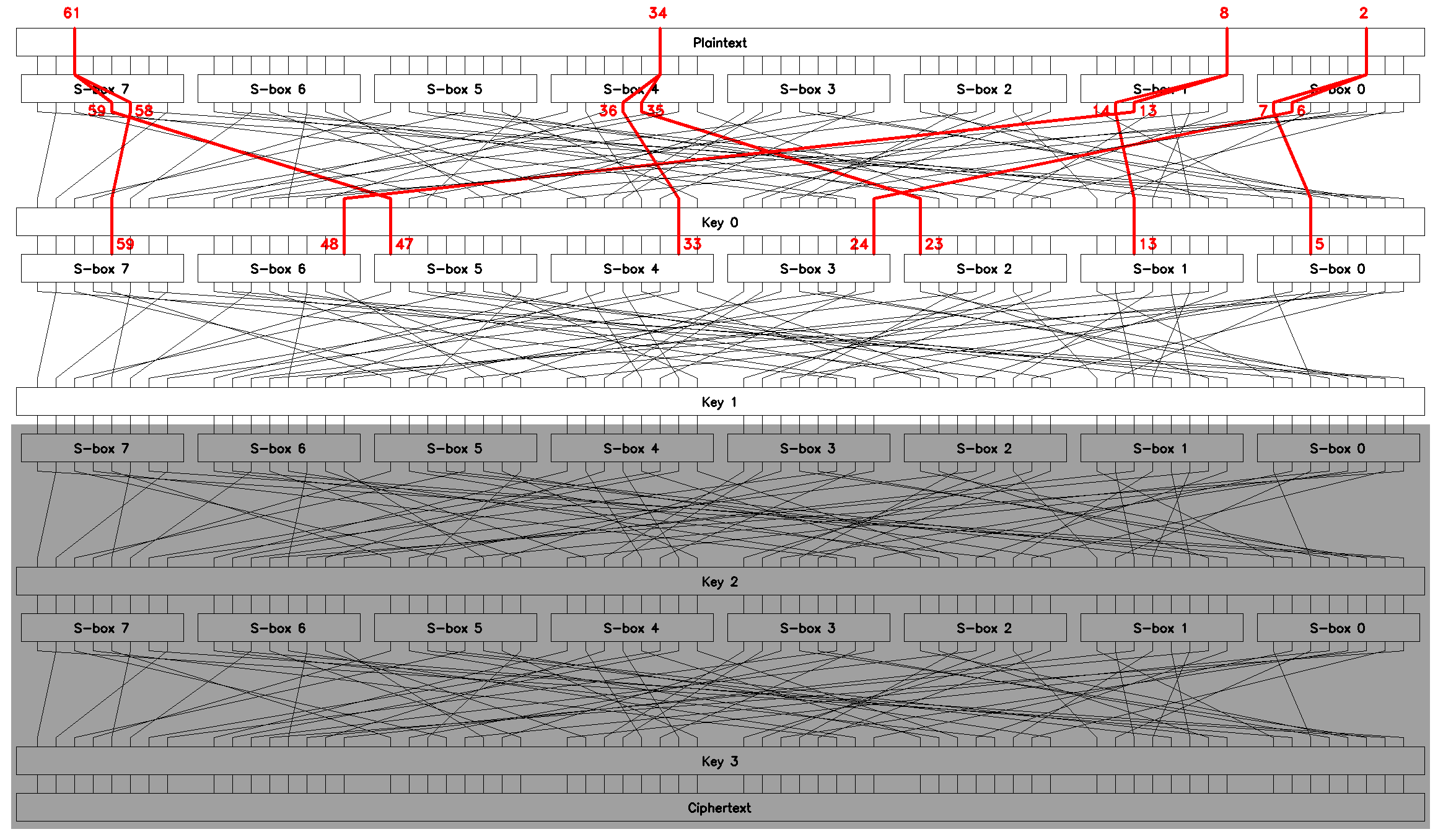
Brute-forcing \(4\) subkeys gives us putative \(K_1\) for a total of \(O\mathopen{}\left(2^{18}\right)\mathclose{}\) operations.
Once again, the reader is challenged to update the linear approximations in function attack_round_three to brute-force the keys \(K_2\) and \(K_1\). Take a look at functions attack_round_two and attack_round_one in the solution script solution.py.
Should everything be done right, the above-mentioned functions will return the correct round keys \(K_2 = \mathrm{0xe102b1cbe4ecb17b}\) and \(K_1 = \mathrm{0x458e3e9ff4e9c6bb}\).
|
Brute-forcing the round keys \(K_2\) and \(K_1\) we found:
|
7. Deducing the first round key \(K_0\) and decrypting the flag
Knowing putative keys \(K_3\), \(K_2\), and \(K_1\), we can decrypt all but the first round of encryption, so the task becomes breaking one-round version of SPlin.
This doesn’t require brute-forcing as the key \(K_0\) can be found directly:
where \(D_{K}(c)\) is one-round decryption of a ciphertext block \(c\) with key \(K\).
The reader is challenged one more time to implement this calculation, see function attack_round_zero in the solution script solution.py.
Finally, with all the round keys known we can decrypt the flag:
225
226
227
228
    with open('flag.txt.enc', 'rb') as f:
        ciphertext = f.read()
    flag = decrypt(ciphertext, keys)
    print('Decrypted flag: %s' % flag)
which outputs
Decrypted flag: b'VolgaCTF{Th0se_s6oxe$_w3re_too_bi@sed}'8. TL;DR
Greetings everyone decided to skip the long narrative and get to the point! Let’s walk through the steps of the implied solution.
First of all, studying the given files we find that:
-
SPlinis a block cipher based on an SP-network [1] with \(4\) rounds, \(64\)-bit block size, and \(256\)-bit key, -
\(256\) bits of a key are split into four \(64\)-bit round keys,
-
data are encrypted in CBC-mode [2],
-
function
check_encryption_filehints at linear cryptanalysis, -
the missing plaintext that corresponds to the given ciphertext file
test.bin.enccan be regenerated, which gives us \(N_p = 35145\) known plaintext-ciphertext pairs.
Then, analyzing the S-boxes SBOX0-SBOX7 we indeed find a lot of linear approximations, some of which are definitely artificial (as their bias values are greater than \(0.4\)).
Eyeballing, we build chained linear approximations that allow us to brute-force the round key \(K_3\), e.g. the four equations shown in Figure 17.
Having found putative \(K_3 = \mathrm{0x3564ea65bcbd493e}\) we move these linear approximations \(L_1..L_4\) up one round, decrypt the last round of encryption for every known ciphertext block \(c\), and perform the same brute-force search for key \(K_2\).
With putative key \(K_2 = \mathrm{0xe102b1cbe4ecb17b}\) we repeat the process once again: move approximations one round up, decrypt one more round of encryption, and brute-force the key \(K_1 = \mathrm{0x458e3e9ff4e9c6bb}\).
To find the only round key left unknown, \(K_0\), we use the keys \(K_3..K_1\) and calculate
This should give us \(K_0 = \mathrm{0x8c4d19320c5d84f7}\).
With all the round keys we can try to decrypt the flag to get
Decrypted flag: b'VolgaCTF{Th0se_s6oxe$_w3re_too_bi@sed}'which is the flag!
References
-
[1] https://en.wikipedia.org/wiki/Substitution%E2%80%93permutation_network.
-
[2] https://en.wikipedia.org/wiki/Block_cipher_mode_of_operation#CBC
-
[3] Matsui, Mitsuru. "Linear cryptanalysis method for DES cipher." Workshop on the Theory and Application of of Cryptographic Techniques. Berlin, Heidelberg: Springer Berlin Heidelberg, 1993. DOI link.
-
[4] Swenson, Christopher. Modern cryptanalysis: techniques for advanced code breaking. John Wiley & Sons, 2008. link
-
[5] Heys, Howard M. "A tutorial on linear and differential cryptanalysis." Cryptologia 26.3 (2002): 189-221. link
-
[6] Joux, Antoine. Algorithmic cryptanalysis. CRC press, 2009.
-
[7] Ohta, Kazuo, Shiho Moriai, and Kazumaro Aoki. "Improving the search algorithm for the best linear expression." Advances in Cryptology—CRYPT0’95: 15th Annual International Cryptology Conference Santa Barbara, California, USA, August 27–31, 1995 Proceedings 15. Springer Berlin Heidelberg, 1995.